Article

Dominant Factors in the Temporal and Spatial Distribution of Precipitation Change in the Beijing–Tianjin–Hebei Urban Agglomeration

1
Key Laboratory of Coastal Science and Integrated Management, First Institute of Oceanography, Ministry of Natural Resources, Qingdao 266061, China
2
Key Laboratory for Earth Surface Processes of the Ministry of Education, College of Urban and Environmental Sciences, Peking University, Beijing 100871, China
3
College of Earth and Environmental Sciences, Lanzhou University, Lanzhou 730000, China
*
Author to whom correspondence should be addressed.
These authors contributed equally to this work.
Remote Sens. 2022, 14(12), 2880; https://doi.org/10.3390/rs14122880
Submission received: 11 April 2022 / Revised: 5 June 2022 / Accepted: 10 June 2022 / Published: 16 June 2022

Abstract

:
Urbanization has a significant influence on precipitation, but existing studies lack the spatial and temporal heterogeneity analysis of its impact on precipitation in urban areas at different levels. This study investigates the spatial heterogeneity of precipitation and the influencing factors on six dimensions in 156 urban areas in the Beijing–Tianjin–Hebei urban agglomeration from 2000 to 2018, utilizing a mixed-methods analytical approach. The results show that the change in the natural factor layer caused by urbanization was the most important factor, affecting urban precipitation variation in summer and over the whole year, accounting for 34.5% and 10.7%, respectively. However, the contribution of the urban thermal environment in summer cannot be ignored, and the change in the urban thermal environment caused by human activities in winter is an important influencing factor. When considering the optimal combination of factors, relative humidity was shown to be significant in the spatial variations in precipitation during summer, which contributed 26.2%, followed by human activity as indicated by night-time light intensity. Over the whole year, aerosol optical depth makes the substantial contribution of 21.8% to urban precipitation change. These results provide benchmarks for improving the adaptability of urban-environment change and urban planning in the context of urbanization.

1. Introduction

With the development in the urbanization process, the urban population has increased greatly as a proportion of the total population, and is expected to be as high as 70% by 2050 [1]. The urban population in China currently stands at about 56.1% of the total and will exceed 70% by 2030, making it one of the fastest-urbanizing countries in the world. The rapid process of urbanization has greatly changed the original natural environment, with changes in surface albedo, evapotranspiration, the moisture of the soil, the degree of roughness of the surface, land–gas flux exchange, energy, and the water cycle, which have a significant impact on atmospheric precipitation [2,3,4,5,6,7,8,9,10].
Since urban areas are home to the vast majority of the world’s population, variation in urban climate and environment will substantially affect the well-being of a great many people. For example, urbanization may increase the probability of extreme precipitation in some cities [1,11,12,13,14,15]; it may also reduce the precipitation effect in cities [16,17], thereby heightening residents’ risk of exposure to extreme weather events [18,19,20,21,22]. Hence, evaluating the impact of urbanization on precipitation change is of the utmost importance in urban climate research [7,23], and, in recent years, domestic and international attention has begun to be paid to the relevant impacts of urbanization precipitation on urban drainage and water-logging prevention [24,25,26,27], urban water-resource management [28,29,30,31,32], municipal traffic [25], the ecological environment [26,33], and even human health [12,34,35]. Great efforts have been made to identify appropriate countermeasures in the form of adaptation and regulation [2]. Therefore, exploring the precipitation effect of urbanization and determining the leading factors in different seasons is crucial for improving the adaptability of urban-environment change and urban planning, and for promoting the sustainable development of urban areas and improvements in well-being [36,37].
Many experts have carried out studies on the precipitation effect of urbanization. Site observation data provide evidence that urban expansion has a substantial impact on precipitation from a statistical perspective, and scholars have found that urbanization increases downwind precipitation in cities [1,12,38]. Drawing on satellite and remote-sensing data, researchers have shown that urbanization increases the intensity of urban precipitation [39] and the probability of urban flood [40,41,42]. In addition, numerical model simulations have been used to explain the mechanism of the precipitation effect of urbanization [40,43,44], with scholars arguing that urbanization is the likely cause of changes in net radiation, latent heat, sensible heat, albedo, frictional rate and boundary-layer height in urban areas that lead to variation in the intensity and location of urban precipitation [40,45,46].
However, most existing research has been conducted in the form of case studies on a single city [36,47,48] or simulation studies of the effect of urbanization on heavy rainfall [40,48]; the results are neither convincing nor representative. Studies on the differences between cities or urban agglomerations [49,50] are often carried out on the basis of the same level of cities, and lack statistical evidence at different scales of development (small, medium, and large). Moreover, there have been few studies on the influence of urban morphology on precipitation. To address these research gaps and to achieve an objective and comprehensive evaluation of the urbanization effect on precipitation, it is necessary not only to take account of samples that have sufficient quantity and spatial heterogeneity, but also to consider urban morphology, urban development and natural elements, air pollution, and the urban thermal-environment factor.
Therefore, this study uses 156 urban areas of different sizes from the Beijing–Tianjin–Hebei (or Jing-Jin-ji) urban agglomeration (BTHUA) to explore the impact of the development of urbanization on urban precipitation change from 2000 to 2018. The BTHUA is an appropriate sample for exploration for several reasons. First, most of the cities in the BTHUA are located on the North China Plain, and their climate types can be categorized in terms of a temperate monsoon season with the same periods of rain and heat; generally, there is little difference in their climate backgrounds (compared with other regions in China, which have complex and diverse climate types), and the geographical spatial scale is also moderate. Second, coverage of large, medium, and small cities provides an effective way to assess the impact of urban development on precipitation. Third, the rapid urban development of recent decades has resulted in a high degree of agglomeration and expansion in some areas, and the rapid expansion of small and medium-sized towns has led to huge changes in urban boundary morphology [51]. This makes it possible to provide a variety of morphological indexes and is conducive to the assessment of the impact of urban morphology on precipitation.
The purpose of this study is to address the following two research questions: (1) What are the dominant factors that affect precipitation change in the process of urbanization in the BTHUA? (2) Does urban morphology have an impact on precipitation or not? The results are expected to provide a benchmark for strategies to adapt to climate and environmental change during the process of urbanization.

2. Materials and Methods

2.1. Study Area

The BTHUA, with a total of 156 urban areas, includes Beijing, Tianjin, and 11 prefecture-level cities in Hebei Province (Baoding, Langfang, Shijiazhuang, Tangshan, Handan, Qinhuangdao, Zhangjiakou, Chengde, Cangzhou, Xingtai, and Hengshui) (see Figure 1). According to the 2018 Statistical Yearbook data of Beijing–Tianjin–Hebei, the BTHUA has a permanent population of 112.7 million and an economic output of CNY 8.4 trillion. Its per capital GDP is 1.3 times the national average, making it one of the three engines of economic development in China. Since the beginning of the twenty-first century, the BTHUA has undergone a rapid process of urbanization expansion. From 2000 to 2018, the urban area of the BTHUA has increased by 9450.77 km2, which was 2.5 times the growth rate of 1980–2000. During this process of rapid urbanization, changes in air quality [52], urban form [51,52,53], urban heat islands [51,53,54], and underlying surface [42,55] have had a significant impact on water vapor and the urban energy balance, and thus an impact on local precipitation. The BTHUA contains sizable town areas which are among the fastest-growing areas of urbanization in China. Therefore, studies conducted on the effect of urbanization on precipitation in that region, and explorations of the relationship between different factors and precipitation there, will provide a basis for urban-development planning and climate-change adaptation strategies not only for the BTHUA but also for other agglomerations in China.

2.2. Data Sources

2.2.1. Selection of Variables

Different typical variables were selected from six dimensions: urban morphology, urbanization development level, natural/climatic background, land surface attributes, air quality, and urban thermal environment (Table 1). The three factors selected to represent urban morphology are FRAC (the fractal dimension index), CIRCLE (the circle index), and CONTIG (the contiguity index). For level of urbanization development, the three indicators are POP (urban population density), NLI (nighttime light intensity), and AREA (urban area size). The four factors representing natural factors are WIN (wind speed), RHU (relative humidity), RAD (radiation), and ALT (average altitude of the city). NDVI (normalized difference vegetation index) and TREE (tree cover) were taken as indications of surface condition, and AOD (Aerosol optical depth) and PM2.5 (Particulate matter with a diameter of less than 2.5 microns) represent urban air quality. Two indexes of UHI (urban heat island) and LST (land surface temperature) represent changes in the thermal environment caused by urbanization. These factors were selected for inclusion on the basis of the following considerations.
Urban morphology factors, such as FRAC, CIRCLE, and CONTIG, affect not only WIN but also UHI, which, in turn, has an effect on the stability of the atmosphere. According to research carried out by Liang et al. [51,53], the more complex the fractal dimension, the greater the roundness and continuity; the less favorable the urban heat dissipation, the stronger the UHI. Furthermore, the contribution to UHI increases with city size. The increase in the urban population and the expansion of the urban area are significant factors in measuring urbanization [51]. The higher the population density per unit area, the greater the anthropogenic heat emitted by human production and living. Urban area expansion affects changes in the latent heat, the sensible heat, and the Bowen ratio of a city [40], and these effects change the heat balance of the city’s atmosphere. NLI is a good representation of human footprint, as it captures the intensity and breadth of human activities and regional development, and it provides spatial information and attribute information [55,56,57]. The higher the NLI value, the greater the surface modification due to human activities. Wei et al. [55] proved that changes in POP, AREA, NLI, and the interactions of other factors all increase influences on urban precipitation change.
Generally speaking, the greater the RHU, the greater the probability of condensation under appropriate conditions. Expansion of urbanization leads to the dry-island effect [58], which results in more obvious vertical gradient of atmospheric humidity over cities (drier at the lower levels and wetter at the upper levels) [59], thus affecting urban precipitation. Wind affects urban heat dissipation and pollutant diffusion, among other factors [60]. NDVI, which denotes the growth potential of vegetation, and TREE, which stands for urban forest coverage, together represent the transpiration of vegetation, which has an important influence on changes in atmospheric relative humidity and surface temperature [61]. The higher the net radiation (RAD) input to the surface, the more the heating effect on the surface increases atmospheric instability and triggers convective precipitation [40].
The higher the altitude, the more complex the change in water-vapor combination may be [14]. In the process of rising, airflow more easily condenses into clouds, causing rain [14]. AOD and PM2.5 are condensation nuclei, and their levels influence precipitation [62,63]. Studies have shown that increases in AOD and PM2.5 concentration reduce the impact efficiency of atmospheric water droplets, making them more uniform and reducing the probability of light rain [17]. However, with the development of deep convection, an increase in AOD and PM2.5 concentration may increase the probability of heavy rain [17]. The UHI can reflect the stability of the urban surface atmosphere. The stronger the UHI, the more unstable the surface atmosphere and the more easily convective precipitation is triggered [54,64]. Due to the strong spatial heterogeneity of the underlying surface types between cities and suburbs in different regions, the higher LST of cities may mean the higher atmospheric temperature near the surface; however, because UHI is mainly related to temperature discrepancies between cities and suburbs, this may not necessarily enhance the heat-island circulation between the two.
The BTHUA has a typical temperate monsoon climate, with high temperatures and rain in summer, being cold and dry in winter, and with the rainy season mainly concentrated in June, July, and August. Accordingly, this study mainly analyzed the relationship between urbanization and precipitation changes in summer (June, July and August) and winter (December, January and February) (while spring and autumn were not analyzed).

2.2.2. Data Sources for Different Variables

Based on the 30 m land use data (https://www.resdc.cn/data.aspx?DATAID=283) (accessed on 1 September 2020) in different periods in 2000, 2005, 2010, 2015 and 2018, we selected 51 categories in the secondary land use classification to calculate the urban form indexes, such as FRAC, CIRCLE, and CONTIG. The calculation of these urban form indexes was completed in version 4.2 of Fragstat software(http://www.umass.edu/landeco/research/fragstats/downloads/fragstats_downloads.html#FRAGSTATS, accessed on 1 June 2019). The calculation formula is shown in Table 1. The aim of this study is to explore the built-up area in 2018, merging and screening the urban boundary and non-urban land patches according to the degree of patch continuity and the influence of the ocean or cities in other provinces; the continuous patches were therefore taken as a research unit, whereas those affected by sea water and inaccurate classification were deleted. This screening and merging process yielded a total of 156 urban areas (Figure 1b), which are independent of each other and continuous in time, and are not affected by the ocean or adjacent patches [51]. NASA’s social and economic statistics (http://sedac.ciesin.columbia.edu/data/set/gpw-v4-population-density-rev10) (accessed on 1 September 2020) were used to obtain the POP of each town unit, at a spatial resolution of 1 km, and AREA was calculated in terms of the space occupied by urban patches in the land use data for each period. NLI was taken as the average night light-intensity index for each town unit according to the annual composite data collected using DMSP-OLS sensors. The spillover effect enhances the spatial distribution continuity of the data, which does not accurately reflect the spatial distribution characteristics of the intensity of human activities, because the brightness of night light does not increase with an increase in human activities after the maximum has been reached. Therefore, the DMSP nighttime light data used here were calibrated and corrected in time sequence [57], at a spatial resolution of 1 km, and the NLI for 2018 was obtained using the linear interpolation method. The meteorological data used in this study (RHU, WIN, and RAD) were taken from the historical monitoring data of the National Meteorological Center of China (http://data.cma.cn/data/detail/dataCode/A.0012.0001.html) (accessed on 20 September 2020), and the spatial grid was obtained via ordinary kriging interpolation, further extracted by resampling according to the boundary of each urban unit. The air pollution data are the latest made available by NASA (http://sedac.ciesin.columbia.edu/data/set/gpw-v4-population-density-rev10) (accessed on 1 September 2020), at a spatial resolution of 1 km.
Since our research objects include small cities and relatively dense towns, 1 km resolution provides enough spatial detail for comparison. Urban vegetation characteristics were drawn from two kinds of remote-sensing data, including the normalized difference vegetation index from the annual 1 km resolution synthetic NDVI data (https://lpdaac.usgs.gov/dataset_discovery/modis/modis_products_table/mod13a3_v006) (accessed on 1 September 2020). Tree cover data were taken from the MODIS vegetation continuous fields (MOD44B, Vegetation Continuous Fields Yearly L3 Global 250 m) (https://modis.gsfc.nasa.gov/data/dataprod/mod44.php) (accessed on 1 September 2020). The land surface-temperature data were derived from the monthly composite surface temperature of the DIDLT1M product in the geospatial data cloud (http://www.gscloud.cn/sources/accessdata/336?pid=333/) (accessed on 20 September 2020), at a spatial resolution of 1 km, and the urban heat island was calculated in terms of the differences between urban and suburban average temperatures. Since the BTHUA has expanded during the 18 years under study, it is important to ensure comparability between the intensity of the urban heat-island effect in different years and seasons. Here, the urban boundary of 2000 was selected for the calculation of the average urban LST. Taking account of the buffer zone built up outward from the urban boundary in 2018 with a width of 10 km (based on the size of urban areas) [51,55], the suburban LST was obtained by calculating the average land-surface temperature within the buffer zone. The surface UHI was calculated by subtracting the suburban average temperature from the urban LST. All the selected variables (Table 1) above were extracted from the data of the five periods of 2000, 2005, 2010, 2015 and 2018, with precipitation as the dependent variable and other selected factors as independent variables for analysis. In order to exclude the impact of climate change and reflect the impact of urbanization, the value of each factor in this study was the difference between the corresponding factors of cities and suburbs (except for the data of elevation, urban form and area).

2.3. Methodology

The methods used in this study were the partial least squares method, stepwise regression, optimal subset regression, and hierarchical regression (HR). Stepwise regression made it possible to look at the effects of each stratification factor. The partial least squares method was used to judge whether each factor of the chosen and the urban precipitation correlation, for the existence of significant correlation factor, enters the full subset regression. HR was then used to analyze the output results of the optimal subset regression. The importance of the influence factor on the change in precipitation was assessed according to the changes in R2. These methods are described in detail in Section 2.3.1, Section 2.3.2 and Section 2.3.3.

2.3.1. Partial Least Squares Method and Stepwise Regression Analysis

We conducted a partial correlation analysis between different selected variables and precipitation before analyzing. The analysis results showed that different variables were related to precipitation. Before analyzing the data, the selected elements were first tested for collinearity, and the variance inflation factor (VIF) was determined. When 0 < VIF < 10, there is no multicollinearity; when 10 ≤ VIF < 100, some multicollinearity is present; when VIF ≥ 100, there is severe multicollinearity. Our analysis established that the VIF of all the elements was less than 1.5, which indicated that there was no multicollinearity in the selected factors. To prepare for the next multiple regression, based on the partial least squares method (OLS), and taking precipitation as the dependent variable and each factor as the independent variable, the factors that passed the 95% (p < 0.05) significance test were taken as the important influencing factors of urban precipitation in different seasons. In each indicator dimension, we used stepwise regression analysis (this study adopts the “entry” model) and a collinearity test (VIF less than 1.5) to calculate the comprehensive explanatory rate of each stratified factor of the impact of urbanization on precipitation in each season.

2.3.2. Optimal Subset Regression

Although stepwise regression can yield the best regression model, it introduces the influencing factors into the regression equation separately according to their significance without considering all their possible combinations [65]. To overcome this limitation, the optimal full subset regression model was used in this study. This method not only takes into account all possible combinations of explanatory variables but also provides more information about factor combinations. It has been shown to be reliable [66] and has been applied widely [67,68,69,70,71]. Using the R-LEAPS software package (https://www.r-project.org/) (accessed on 30 December 2020), we constructed all possible combination models from the impact factors that passed the significance test in OLS. We set the value of N-best (the number of output optimal models) to 1; that is, every time the number of independent variables changed, an optimal regression model that passed the significance test was generated accordingly. Then, we assessed the model fit in terms of the adjusted R2; the larger the adjusted R2, the better the model. Since the adjusted R2 values of some of the best models were very similar, we used the Mallows CP information standard value as the judging standard and the minimum Mallows CP value to determine the optimal model.

2.3.3. Hierarchical Regression Analysis

For each impact factor entering the optimal subset regression model, we used the HR method to determine the independent impact of explanatory variables contained in the optimal model. The HR method is based on semi-parametric regression analysis and calculates the relative importance of each factor by performing multiple random transformations on the original data matrix. The advantage of this method over traditional regression analysis is that it overcomes common collinear phenomena in environmental variables, which makes it particularly suitable for multidimensional environmental data analysis [72]. In this study, we obtained the independent importance from the changes in R2 for each factor according to the results of the HR analysis; the greater the change in R2, the stronger the influence of the variable on the change in precipitation. Then, we ranked the changes in R2 to determine the dominant factors affecting urban precipitation in different seasons.

3. Results and Analysis

3.1. Temporal and Spatial Patterns of Precipitation

3.1.1. Spatial Distribution Characteristics of Precipitation Changes in Different Seasons in the BTHUA

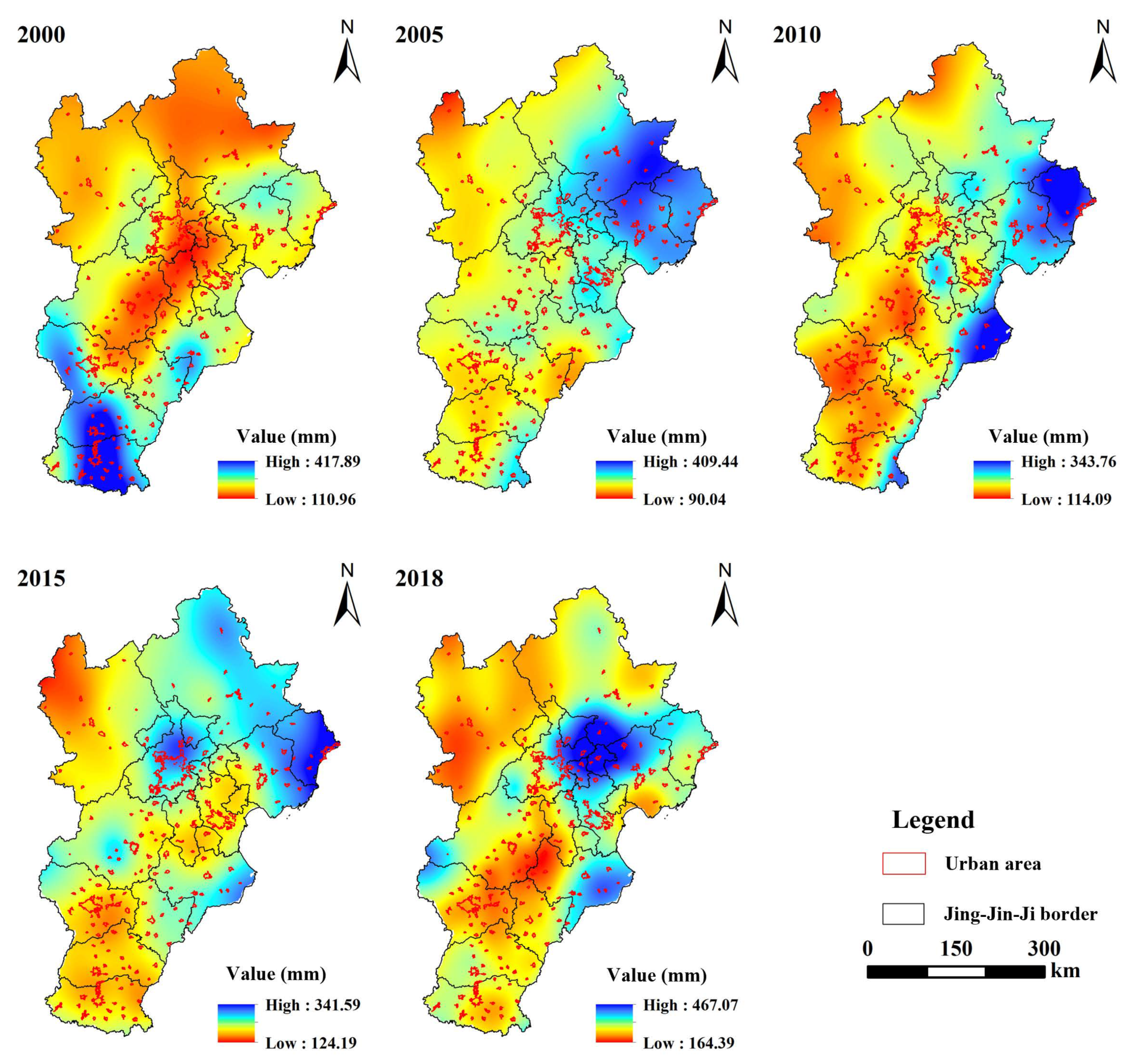
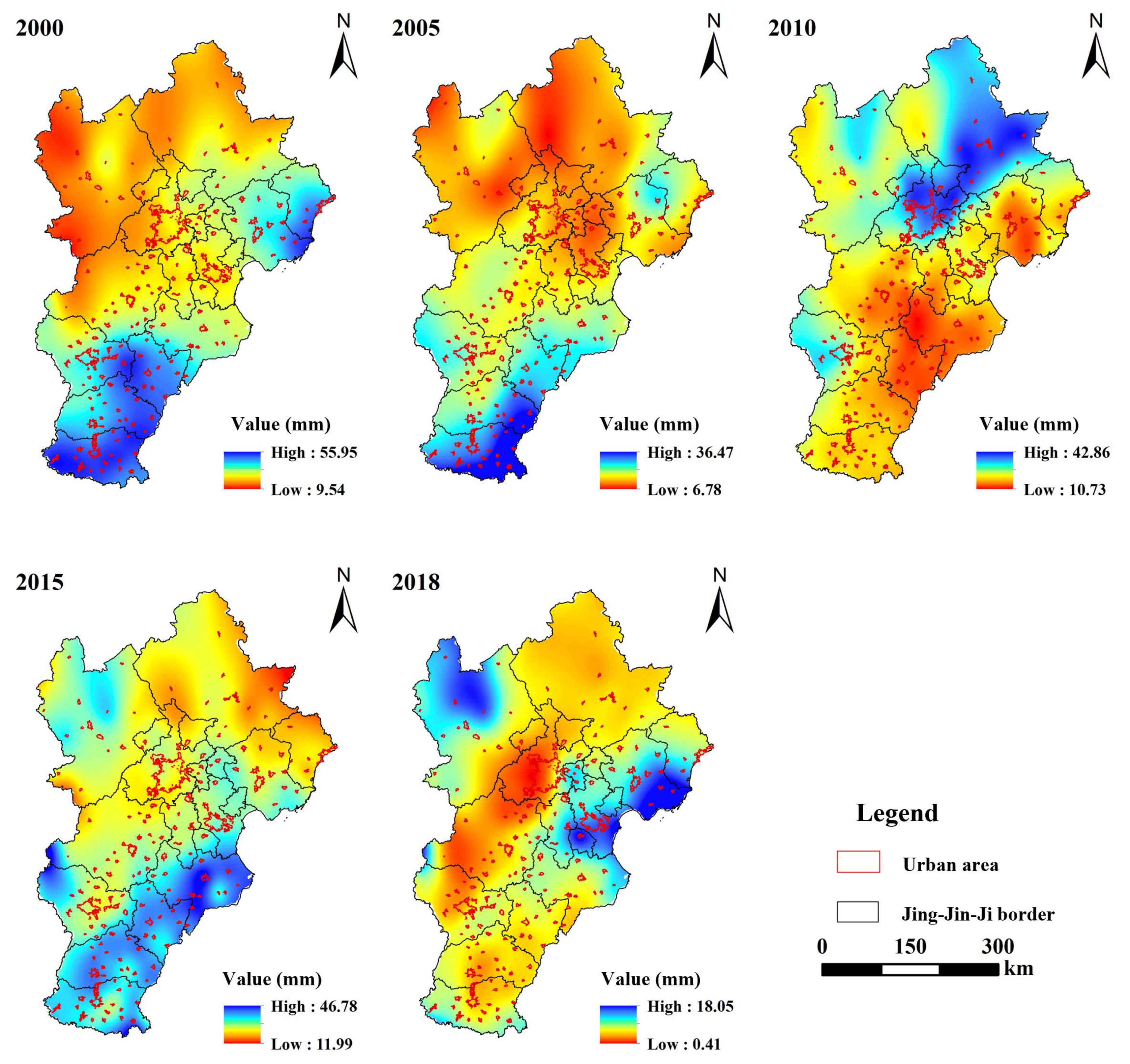
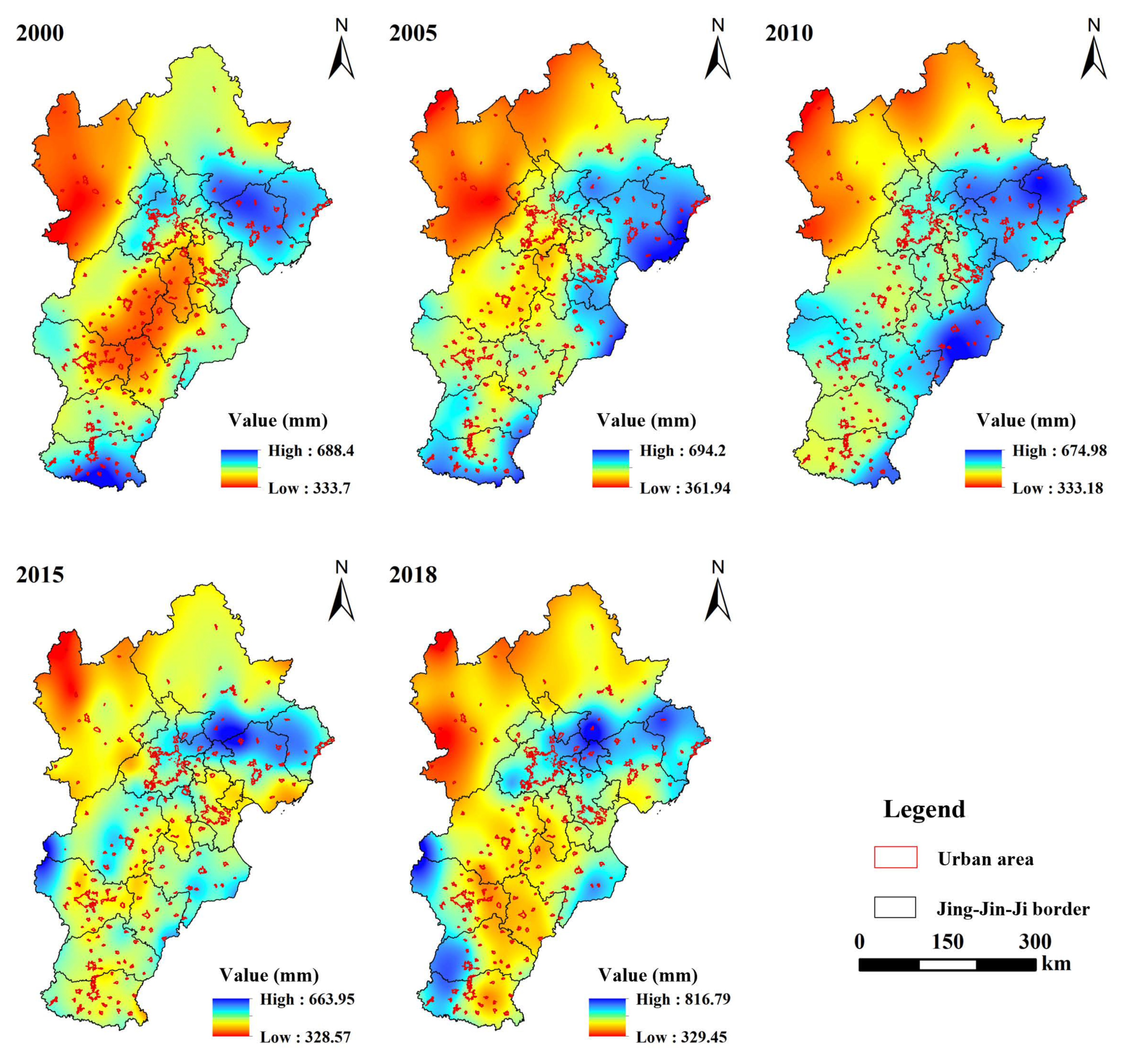
In this study, the ANUSPLIN software (https://fennerschool-anu-edu-au.translate.goog/research/products/anusplin?_x_tr_sl=auto&_x_tr_tl=en&_x_tr_hl=zh-CN&_x_tr_pto=wapp) (accessed on 30 December 2020) was used to interpolate the precipitation data of more than 2400 meteorological stations in China; in addition, the BTHUA boundary was used as a mask to extract the spatial distribution of precipitation in different urban areas in the BTHUA (the spatial resolution is 250 m × 250 m). It can be seen from Figure 2, Figure 3 and Figure 4 that there were seasonal and spatial differences in the changes of precipitation in the BTHUA from 2000 to 2018. In summer, precipitation tends to increase in the northern part of the BTHUA, especially in the northern and northeastern parts of Beijing. In the southern part of the BTHUA, precipitation tends to decrease in summer, winter and throughout the year. In winter, the increase in precipitation was mainly distributed in the northwest Zhangjiakou area (Figure 3).
It can be derived from the perspective of annual precipitation changes (Figure 4) that the increase and decrease in distribution areas of precipitation were roughly consistent with the spatial distribution characteristics of summer precipitation changes. Judging from the spatial distribution characteristics of precipitation changes in different seasons, areas with large precipitation changes were often related to more urban units contained in the area. For example, the area around the Beijing megalopolis had become an area with a large increase in summer precipitation. Therefore, it can be concluded that this may be related to the influence of changes in water vapor and heat balance caused by urbanization on atmospheric precipitation.
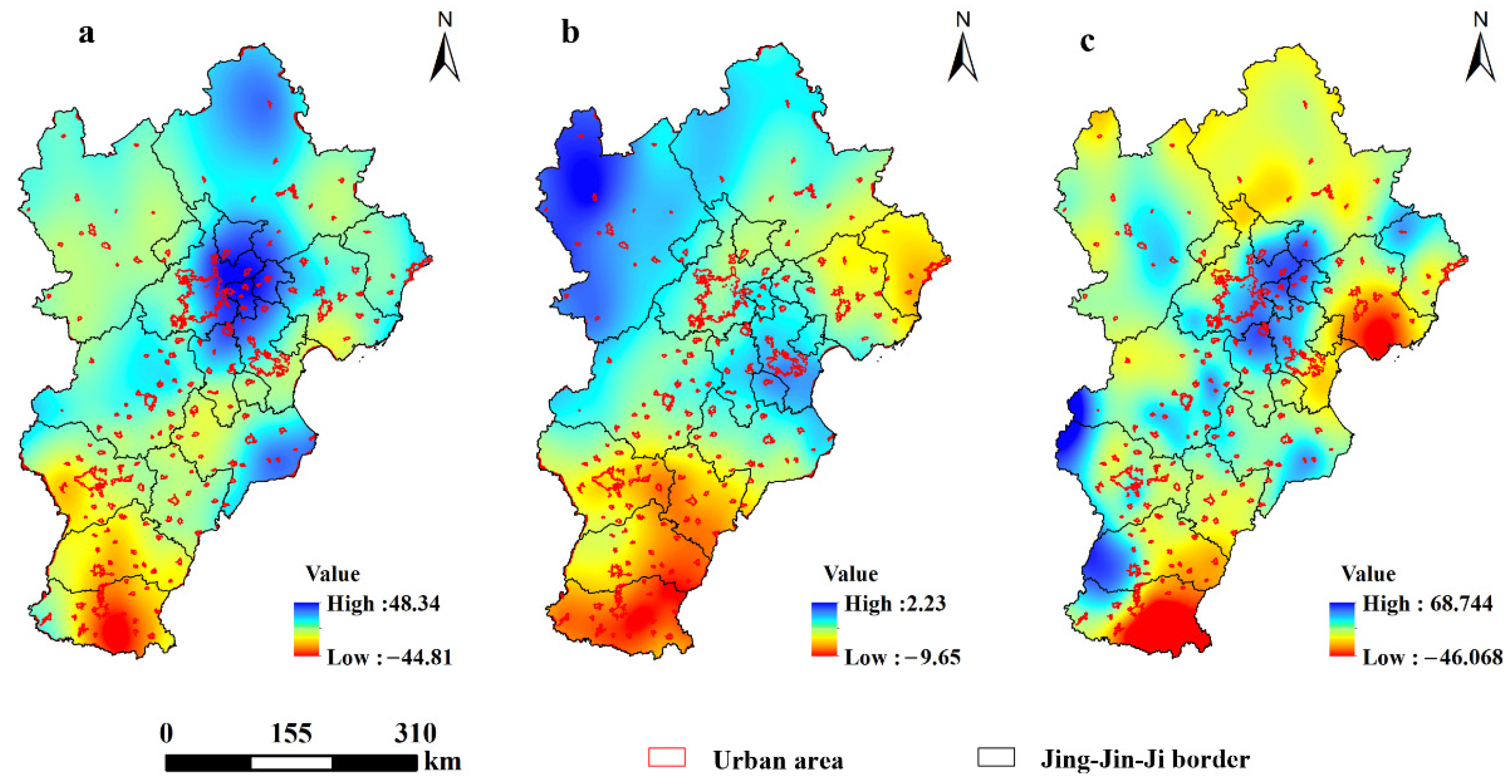
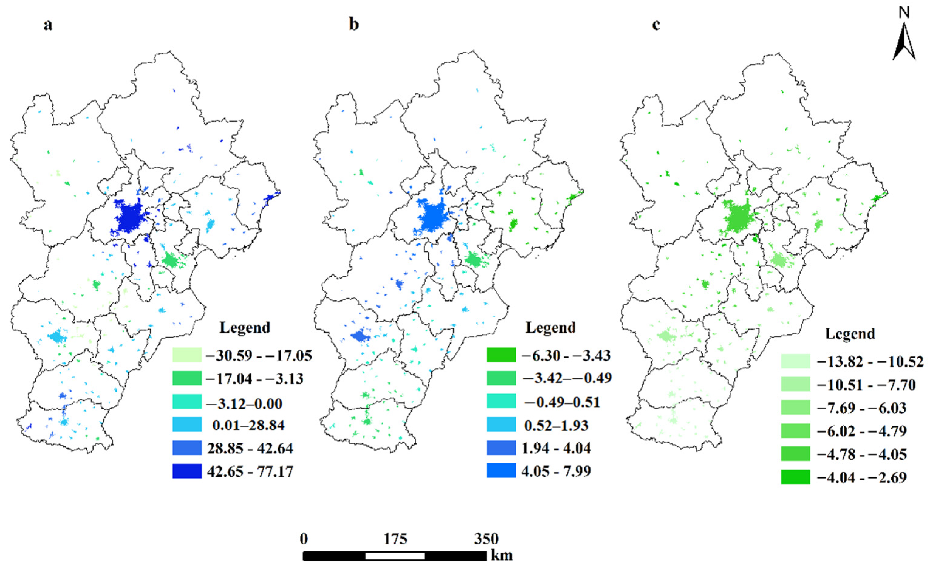
From the perspective of precipitation change rate (Figure 5), it can be clearly seen that, although the average precipitation in the southern part of the BTHUA (such as Handan and Xingtai, etc.) was higher than that in the northern part (such as Beijing, etc.) during 2000–2018, the precipitation in the region showed a decreasing trend no matter whether in summer, winter or throughout the year. Similar situations were also to be seen in Shijiazhuang, Tianjin and Tangshan. The spatial distribution of areas with precipitation increases in different urban areas in summer and throughout the year was generally similar, which were mainly distributed in Beijing, Zhangjiakou, Chengde, the northeast of Qinhuangdao, Baoding and Cangzhou urban areas and its surrounding town areas. Due to the different data sources, research methods and the size of the study area, although the results of this study cannot be directly compared with many existing studies on the whole, it is to be observed that, in the study of the areas with overlapping parts such as Beijing, the precipitation changes in this study were consistent with some existing research conclusions [73,74,75]. In winter, the areas with increased precipitation were mainly distributed in Beijing and northern regions, and some urban areas in the Hengshui–Cangzhou region.

3.1.2. Spatial Distribution of Urban Precipitation Changes in Inner Urban Areas of Different Cities in the BTHUA

In order to evaluate the changes in urban precipitation caused by urbanization, this section utilized the urban boundary in 2000 to extract the average precipitation per unit area of different cities in each period, and adopted the precipitation extracted from the 10 km buffer area outside the urban unit boundary in 2018 as background values. Then, the average precipitation within the urban unit boundary in 2000 was subtracted from the average precipitation in the suburbs outside the 10 km buffer zone of the urban unit boundary in 2018 to obtain the impact of urbanization. The main purpose of this approach was to ensure that, during the study period 2000–2018, urban areas were always cities, and suburban areas were always suburbs, so that the impact of urbanization on precipitation in different periods can be compared. On the basis of the above results, this paper used the trend analysis method to calculate the change rate (slope) of urban precipitation in different cities from 2000 to 2018 (the fifth period). The results are shown in Figure 6. On the whole, the change trend of precipitation in the inner city of the BTHUA was not very obvious (the coefficient is −0.012, p < 0.000), and the change trend was generally consistent with the findings of Jiang et al. [59]. In summer, the change trend of the difference between the urban area and the background values in the entire BTHUA over time was slightly positive (the coefficient is 0.077, p < 0.000). However, there were large spatial differences in the average precipitation changes in different regions and different seasons.
As shown by Figure 6, the areas with increased precipitation in the inner urban areas in summer were mainly concentrated in the larger urban areas of Beijing, Zhangjiakou, small towns in the northeast of Qinhuangdao, Shijiazhuang, Xingtai and some small towns in the south of Handan. The areas with reduced precipitation were mainly distributed in cities and towns such as Baoding and Tianjin. In winter, the areas with slightly increased precipitation were mainly distributed in the urban area of Beijing (consistent with the results of Song et al. [75]), the urban area of Baoding and Shijiazhuang and its surrounding areas, while in Tianjin, Tangshan, Qinhuangdao and the towns of Handan and Xingtai in the south, the precipitation showed a decreasing trend. On the annual scale, relative to the background value, the precipitation in different cities and towns in different seasons showed a decreasing trend. The areas with a significant decrease were mainly located in the southern region, and the northern region had a relatively small decrease, showing a slower decrease trend from south to north. It is worth noting that the precipitation changes in spring and autumn were not considered in this study, and the precipitation changes showed a decreasing trend on the annual scale, which may be caused by the difference in precipitation between inner and suburban areas of different cities in spring and autumn. Overall, the above results indicate that, although different urban areas in the BTHUA are adjacent and have similar climatic backgrounds, there were significant differences in precipitation among them, which may be closely related to changes in the natural environment and human activities caused by urbanization. In addition, in the same city, there were differences in the precipitation between the inner city and the suburbs, which showed that urbanization does have a greater impact on the precipitation.

3.2. Significant Influencing Factors on Precipitation

3.2.1. Significant Influencing Factors on Precipitation in the Whole Factor Layers

The stepwise regression results showed that the explanatory power of each factor layer for spatial changes in precipitation in the BTHUA changed accordingly at different times (Table 2). In summer, the explanatory power of the natural factor layer was greatest (34.5%), followed by the urban thermal-environment factor (16.6%), and then by the land surface attribute layer and urban development level (13.2% and 10.3%, respectively). The explanatory power of the urban morphology factor layer was no higher than 1%. Hence, the change in natural factors caused by urbanization is the most important factor affecting the change in precipitation in summer in the BTHUA, consistent with the research findings of Wei et al. [55]. Nonetheless, the impacts of urbanization on urban precipitation, such as changes in underlying vegetation and increases in the urban thermal environment and urbanization level, should not be ignored.
In winter, the explanatory power of the urban thermal-environment factor layer was greatest (22.8%), indicating that changes in the thermal environment in different cities in the BTHUA had the greatest influence on changes in precipitation. The explanatory power of the air-quality factor was 15.9%, and the explanatory power of the natural-environment factor was 14.8%. These results show that changes in air quality and in the natural environment caused by human activities have an important influence on changes in urban precipitation in winter. The impacts of the other factor layers were relatively small or insignificant. Of these, the highest explanatory power belonged to the natural factor layer (10.7%), followed by the level of urbanization development (7.5%). Table 2 shows that the number of factor layers in the stepping-regression model increased greatly over the year, but that the explanatory power of each factor layer tended to decrease. This indicates that the factors affecting the urbanization of the BTHUA for the whole year may be diverse and more complex.

3.2.2. Significant Influencing Factors on Precipitation in Each Factor Layer

Table 2 shows that, in the urban-morphology factor, only FRAC entered the stepwise regression in summer and for the whole year. The explanatory power of FRAC is small (1%) in summer, which indicates that the fractal dimension could affect the change in precipitation in a city. However, compared with other factors, its direct impact was very small and can even be ignored. The explanatory power for the year is greater (5%), which suggests that the fractal dimension may have a substantial influence on precipitation in other months or seasons. At the urban development level, according to the OLS regression, POP did not pass the significance test, regardless of the season, which indicates that the influence of urban population on precipitation change is limited. NLI had a strong influence on precipitation in summer and in winter. As NLI represents the intensity of human activities, this indicates that the greater the intensity of human activities, the more man-made heat is emitted and the more likely it is to cause atmospheric instability in summer, promoting convective precipitation [55]. In winter, AREA did not enter the stepwise regression model for the urban development level, unlike NLI and POP. The maximum R2 of NLI did not account for 50% of the explanatory power of the stepwise regression model of the urban development level. It may be that the interaction between NLI and POP increased, thereby strengthening the explanatory power [55].
In the natural factor layer, RHU had the highest explanatory power in summer and for the whole year. Its explanatory power in summer was 31.4%, accounting for more than 91% of the natural factor layer, which indicates that relative humidity had the greatest influence on precipitation in the natural factor layer in summer. In winter, ALT was the most important influencing factor. As can be seen from the relationship between ALT and precipitation in Table 2, this may be related to the increase in altitude forcing airflow to lift and increasing topographic rain. In the land-surface attribute layer, the explanatory power of NDVI accounted for more than 70% of the land-surface attribute layer in summer, although it did not enter the stepping-regression model for the year. NDVI represents the growth of vegetation; the higher the NDVI in summer, the better the vegetation coverage. Plant evapotranspiration makes available a large amount of water vapor for meteoric precipitation, thereby increasing precipitation.
In the air-quality layer, no factor entered the stepwise regression model in summer, which indicates that the influence of air quality in summer was not very significant. In winter, AOD and PM2.5 both entered the model, and both had a great impact. Over the whole year, only AOD entered the stepwise regression model. The OLS regression results showed that AOD and PM2.5 had negative effects on precipitation change both in winter and for the year. This suggests that, in the case of relative drought or relatively low humidity, if the air pollution is serious (if AOD or PM2.5 increases), then the higher aerosol concentration will distribute the droplets in the atmosphere more evenly, inhibiting the collision and condensation process of water droplets and reducing precipitation. In the urban-thermal-environment layer, the explanatory power of LST for precipitation change in summer and in winter was higher than that of UHI. The explanatory power of LST in winter was 22.6%, accounting for more than 99.1% of the urban-thermal-environment layer, making it the most influential factor on precipitation change in that layer, and the explanatory power of UHI exceeded that of LST over the year. It should be noted that, although there is a certain connection between LST and UHI, high LST does not necessarily mean high UHI, as UHI is related to the disparity of average surface temperatures between cities and suburbs. In general, the stronger the UHI in summer, the stronger the atmospheric instability, which increases precipitation by triggering convective precipitation [12]. However, in winter or in the dry season, an increase in UHI reduces the probability of precipitation [45]. As can be seen from Table 2, these results are similar to the conclusions drawn by most researchers. However, previous studies have tended to consider only the role of UHI, without taking account of the direct influence of LST. When LST was included as the independent variable, the present study found that the influence of LST exceeded that of UHI.
These results demonstrate that a single variable or single-factor layer can have an influence on precipitation change. If multiple elements are jointly affected, then the sign of the relationship between the univariate and the precipitation may change. Therefore, in order to obtain a more realistic relationship between the variables and precipitation, the joint action of multiple variables was adapted to exclude the influence of various factors and to make the results more convincing (see Section 2.3.2 and Section 2.3.3 for details).

3.3. Optimal Regression Model

For different seasons, if the impact factors of urban precipitation passed the significance test (p < 0.05), they were selected as the influencing factors of urban precipitation and included in the full subset regression. As Table 2 shows, nine, ten, and seven important factors entered the regression model in summer, in winter, and for the whole year, respectively. We set NBEST to 1; that is, every time the number of independent variables changed, an optimal regression model that passed the significance test was generated accordingly. Ultimately, there were eight optional models of output in summer that passed the significance test, eight in winter, and seven for the year. Since several optional models had similar R2 values for each season, we chose models on the basis of higher R2. A small Mallows CP value indicates that the model can explain more urban precipitation changes with fewer variables. Therefore, when R2 values were the same, we determined the model with the lowest Mallows CP value as the best for each season.
As shown in Figure 7a–c, six explanatory variables (CIRCLE, NLI, AREA, RHU, NDVI, and LST) entered the optimal model in summer; the adjusted R2 was 0.38, and the Mallows CP value was 6.2. Eight explanatory variables (WIN, RAD, ALT, NDVI, AOD, PM2.5, UHI, and LST) entered the optimal model in winter; the adjusted R2 was 0.30, and the Mallows CP value was 8.6. On the annual scale, five explanatory variables (RHU, ALT, AOD, UHI, and LST) were incorporated into the optimal model, with an adjusted R2 of 0.32 and a Mallows CP value of 5.9. Hence, the number of explanatory variables that entered the optimal model was greater in winter than in summer. This indicates that, when the temperature in the BTHUA decreased, the mechanism of urbanization on urban precipitation change become more complex and more factors were needed to explain the precipitation change. Since we did not consider the influence of urbanization on precipitation change in other months or other seasons in this study, the decrease in the number of explanatory variables in the optimal model throughout the year may also be related to the interaction of various urban elements in other months or other seasons.

3.4. Relative Importance of Precipitation Influencing Factors

In order to observe the importance of the factors affecting urban precipitation more clearly and intuitively, we used the analytic hierarchy process to rank the factors entering the optimal full subset regression model according to changes in R2. The larger the change in the R2 of a factor, the more important the factor’s influence on urban precipitation.
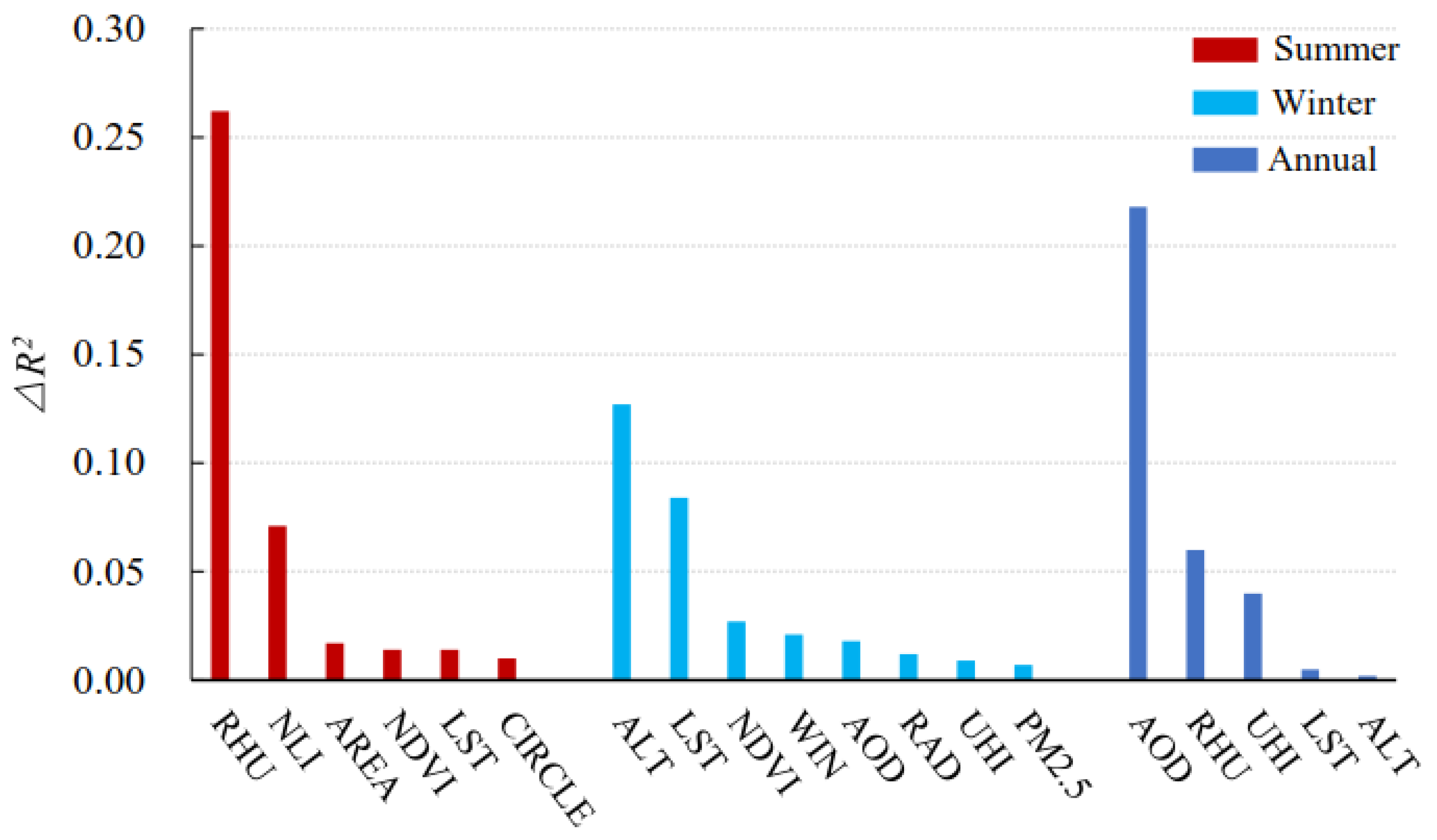
Figure 8 shows the results of entering the optimal full subset regression model in different seasons. Of all the influencing factors considered, RHU in summer made the largest independent contribution (26.2%) to urban precipitation in BTHUA, followed by NLI (7.1%). The values of Area, NDVI, LST, and CIRCLE were 1.7%, 1.4%, 1.4%, and 1%, respectively. ALT and LST made the largest independent contributions in winter, accounting for 12.7% and 8.4%, respectively. The independent contributions of other explanatory variables were as follows: NDVI 2.7%, WIN 2.1%, AOD 1.8%, RAD1.2%, UHI 0.9%, and PM2.5 0.7%. For the whole year, AOD made the largest independent contribution (21.8%) to urban precipitation change in the BTHUA. The independent contributions of RHU, UHI, LST, and ALT accounted for 6%, 4%, 0.5%, and 0.2%, respectively. We can conclude provisionally that, among the influencing factors of urbanization on precipitation in the BTHUA, RHU is the most important factor in summer, ALT is dominant in winter, and AOD is the most important influencing factor for the whole year.
In addition, the independent contribution rate of the dominant factor ranked highest in summer and lowest in winter. The most important factor of the contribution rate between summer and winter for the whole year showed that, when the temperature rises, the change in urban rainfall is more likely to be affected by the dominant factor, and when the temperature falls, the mechanism of the BTHUA urban precipitation becomes more complicated.
The layers of each factor in different seasons, natural factors, and thermal environment all entered the optimal model, but the factors and contribution rates in the model were different in different seasons. Of the natural background layer, only RHU entered the model in summer, and its explanatory contribution was high (26.2%). RHU did not enter the model in winter, but ALT, WIN, and RAD did, and their contribution was 16%. For the whole year, the contribution of the natural background layer accounted for 6.2%. It can be seen that the contribution rate of natural factors to urban precipitation gradually decreased from summer to winter. The contribution of the thermal environment gradually increased from 1.4% in summer (LST) to 9.3% in winter (LST, UHI); for the full year, the contribution was 4.5%. Only in summer did the urban development level and urban form layer factor (CIRCLE) enter the best model. The explanatory power of urban development level factors (NLI, AREA) was 8.8%, second only to the influence of urban natural conditions. This indicates that the intensity of human activities in cities and urban expansion has a significant impact on urban precipitation in summer. Urban morphology factors entered the stepwise regression in summer, and all scales had an impact on the model, but only the CIRCLE factor entered the best subset regression model in summer; nonetheless, its explanatory contribution of 1% suggests that urban-form factor changes can also affect urban precipitation. The land-surface attribute factors had an impact on urban precipitation in summer and in winter, but the impact intensity was not representative in general, and there was no factor that entered into the optimal model for the whole year. Air-quality factors entered the best model only in winter (AOD, PM2.5) and for the year (AOD), with explanatory power of 2.5% and 21.8%, respectively. There is a strong relationship between air quality and atmospheric particulate matter. As condensation nuclei, particulate matter floating in the atmosphere is one of the important conditions for the formation of precipitation, which can increase or decrease the probability of precipitation. Therefore, it was relatively reasonable that AOD had greater explanatory power for precipitation changes throughout the year.

4. Discussion

In terms of urban precipitation from 2000 to 2018 in the BTHUA, the results demonstrate a clear discrepancy in precipitation between different areas in the BTHUA, despite the fact that they are adjacent and that their topographic and climatic backgrounds are similar. These results are of great importance for understanding how urbanization leads to differences between cities in terms of environmental change and the intensity of human activity.
In previous research on the BTHUA, Jiang and Li [59] found that urbanization led to a decreasing trend in urban annual precipitation, similar to annual precipitation trends in some cities. However, their study used statistical analysis to analyze the overall situation of the urban agglomeration, without distinguishing the temporal changes in the spatial areas of each town. Accordingly, more detailed content cannot be provided for the BTHUA. Based on WRF model simulation studies, Wang et al. [76] found that urbanization in Beijing reduced precipitation in urban and suburban areas by 11%. They argued that urbanization increased the impervious layer area, inhibited surface evapotranspiration, reduced relative humidity, and reduced the water vapor cycle of local precipitation. The results in this study are consistent with their findings on changes in relative humidity, which was the dominant factor of precipitation change in the BTHUA in summer. Likewise, Wei et. al. [55], using a geographical probe method to examine the interaction between elements and their influence of urbanization on precipitation, found results for each season that are roughly similar to those of the present study (for example, for RHU in summer, for WIN, AOD, and AOD in winter, and for RHU for the whole year). However, their study considered interactions of two elements only, without taking into account the combined effects among many factors.
Thus, the present study makes a number of novel contributions. In terms of the research content, and unlike traditional single-factor research, it constructs a multi-index system to explore the impact of the urbanization process on precipitation using a specific and comprehensive method. Instead of single-site meteorological data, it takes the city boundary as the inner city in 2000 in order to include the dependent and independent variables in different periods for the years 2000, 2005, 2010, 2015 and 2018. As a result, the independent variable contingency is reduced and the heterogeneity caused by the error is increased, which ensures that the effects of different periods of urbanization on the rainfall are comparable. In terms of research methods, a multiple regression model was established between different factors to eliminate disturbance of the results of the model through the whole subset regression. The city is a complicated coupling system that consists of human and natural elements. Urban precipitation is therefore a complex process that is correlated with many factors and involves many factors in its mechanism, including climate and human activities; however, the intensity of the influence of different factors on precipitation makes accurate measurement and comparison difficult. This study clarifies the effects of various influencing factors of rainfall intensity by computing the contribution rate of the influence of different factors on the precipitation.
The results of this study showed that there were differences in the dominant factors affecting urban precipitation changes in urban areas in different seasons, and the changes in these factors are closely associated with or greatly influenced by human activity and the process of rapid urbanization. Through the analysis of the land-use transition matrix of the BTHUA, we found that, between 2000 and 2018, the urban area of the BTHUA increased by 9450.77 km2, which was 2.5 times the growth rate from 1980 to 2000. In the process of rapid urbanization, the expansion of urban land will lead to the increase in urban impervious area and the decrease in vegetation, and the average surface temperature during the day will also increase; the weakening of urban evapotranspiration will affect the change of relative humidity in the atmosphere. In addition, with the increase in urban population, the intensity of human activities and the emission of pollutants will increase. These processes will finally lead to changes in urban surface latent heat and sensible heat flux, which will affect the stability of the atmosphere. Among these factors, some influence factors (e.g., AOD, PM2.5, and UHI) could be controlled, or humans could curtail certain activities in order to reduce the influence of urbanization on certain elements (e.g., RHU, NLI, and NDVI). Wei et al. [55] showed that, although natural factors such as RHU have a greater impact in summer, human factors such as NLI and UHI are more sensitive and greatly amplify the impact on RHU. Intensification of human activities and increases in UHI are more likely to cause urban atmospheric instability and promote deep convection, which may lead to extreme precipitation. In winter, the RHU is relatively low compared to summer because the wind blows from the land to the ocean. In addition, the increase in coal burning for heating in winter not only increases the AOD in the atmosphere, but also increases the intensity of the UHI, which may increase the condensation saturation of atmospheric water vapor. The combined effect of these factors may reduce the frequency of winter precipitation in the BTHUA (especially light rain), thereby making winter precipitation changes more complicated. Increases in AOD may reduce the probability of light rain (when the relative humidity of the atmosphere is low, the increase in atmospheric pollution will make the water vapor more uniform and reduce the collision efficiency of water droplets, thereby reducing the probability of precipitation), but they increase the probability of heavy and extreme rainstorms [17]. Therefore, during the process of urban development, attention should be paid to the protection of underlying vegetation to reduce the emission of anthropogenic heat and air pollutants, thereby making urban extreme precipitation events less likely. In addition, the urban form (CIRCLE) has become one of the main factors affecting changes in urban precipitation in summer. Therefore, during the process of urbanization, the degree of agglomeration within the city should be subject to reasonable control (that is, the degree of agglomeration should be neither too dense nor too sparse), making it possible to avoid wasting resources.
This study also has certain limitations that should be noted. First of all, this study is based on data analysis for five periods, the years 2000, 2005, 2010, 2015 and 2018. More continuous and complete data that better reflect development trends for different factors are required in order to offer causal explanations. In addition, as urbanization accelerates and human activities intensify, the contributions of different factors are likely to change. This study has not explored the developments and changes in the contribution rates of different factors over time, and this should be the focus of future research. Finally, the goodness of fit (R2) obtained by multiple stepwise regression was not high enough, largely because of the complexity, discontinuity, and strong locality of the precipitation process. Many factors affect precipitation, and the function relationship between natural factors is complex; together with the substantial influence of human activities in the process of urbanization, the roles of various factors, relations, and internal mechanisms are difficult to determine. The present study has identified the general rules and the trend, but a high-precision model is required to study the phenomena more comprehensively and over a longer period.

5. Conclusions

This study explored the correlative relationship between five dimensions of impact factors and spatial changes in different seasons in 156 town areas in the BTHUA from 2000 to 2018. It adopted a mixed-methods analytical approach, using OLS regression, stepwise regression, optimal subset regression, and HR analysis from the perspective of multidimensional indicators for natural and human factors. The provisional conclusions drawn here offer a benchmark for improving adaptability, urban planning, and water-resource management in the BTHUA during the process of urbanization.
First, the change in the natural factor layer caused by urbanization was the most important factor affecting the urban precipitation change in summer and for the whole year, explaining 34.5% and 10.7% of the urban precipitation change, respectively. However, the contribution of the urban thermal environment in summer should not be ignored. In winter, the change in urban thermal environment caused by human activities was the main influencing factor.
Second, in terms of the optimal combination of all factors, RHU, with an independent contribution of 26.2%, was the most important factor affecting spatial changes in precipitation in the BTHUA in summer, followed by NLI, with an independent contribution of 7.1%. These results indicate that changes in the intensity of human activity also have a significant impact on changes in precipitation. The most significant factor in winter was ALT, accounting for 12.7%, but the influence of AOD could not be ignored among the anthropogenic factors in the close relationship with human activities in the city. For the whole year, AOD made the largest independent contribution to urban precipitation change in the BTHUA, as high as 21.8%, followed by the independent contributions of RHU and UHI. The factors affecting precipitation were more complex in winter than in summer. Changes in urban RHU are central to any explanation of the urbanization process in the pad surface NDVI, and NLI, AOD, and UHI are directly related to human activities. Accordingly, attention should be paid to vegetation retention and environment greening in the process of urbanization, in order to reduce seasonal fluctuations of urbanization leading to precipitation change and environmental issues caused by extreme precipitation, and in order to slow down damage to the natural environment as much as possible. Attention should also be paid to controlling emissions of pollutants.
Finally, the results in this study show that urban morphology (CIRCLE) was one of the factors affecting changes in urban precipitation in summer, although its effect was relatively small. Therefore, in the process of urbanization, the degree of agglomeration within the city should be subject to reasonable controls to ensure that it is neither too dense nor too sparse and to avoid wasting resources.

Author Contributions

This manuscript is the result of the research of F.W. under the supervision of S.L. and D.L. and the advising of Z.L., W.M., J.S., Y.W. All authors have read and agreed to the published version of the manuscript.

Funding

This research was funded by the Major Projects of the National Natural Science Foundation of China (grant number 41590843), the Typical Coastal Zone Ecological Restoration Technology and Policy Research (grant number TZ0122001), and the Construction of Key Laboratory of Coastal Zone Science and Integrated Management (grant number GY0221L08).

Acknowledgments

We thank the Major Projects of the National Natural Science Foundation of China (41590843), the Typical Coastal Zone Ecological Restoration Technology and Policy Research (TZ0122001), and the Construction of Key Laboratory of Coastal Zone Science and Integrated Management (GY0221L08) for their support. We are also grateful to the editor and the reviewers for their helpful comments.

Conflicts of Interest

The authors declare that they have no conflict of interest.

References

  1. Zhang, Y.; Pang, X.; Xia, J.; Shao, Q.; Yu, E.; Zhao, T.; She, D.; Sun, J.; Yu, J.; Pan, X.; et al. Regional patterns of extreme precipitation and urban signatures in metropolitan areas. J. Geophys. Res.-Atmos. 2019, 124, 641–663. [Google Scholar] [CrossRef]
  2. Carvalho, D.; Martins, H.; Marta-Almeida, M.; Rocha, A.; Borrego, C. Urban resilience to future urban heatwaves under a climate change scenario: A case study for Porto urban area (Portugal). Urban Clim. 2017, 19, 1–27. [Google Scholar] [CrossRef]
  3. Macintyre, H.L.; Heaviside, C.; Taylor, J.; Picetti, R.; Symonds, P.; Cai, X.M.; Vardoulakis, S. Assessing urban population vulnerability and environmental risks across an urban area during heatwaves—Implications for health protection. Sci. Total Environ. 2018, 610, 678–690. [Google Scholar] [CrossRef] [PubMed] [Green Version]
  4. Mendez-Lazaro, P.A.; Perez-Cardona, C.M.; Rodriguez, E.; Martinez, O.; Taboas, M.; Bocanegra, A.; Mendez-Tejeda, R. Climate change, heat, and mortality in the tropical urban area of San Juan, Puerto Rico. Int. J. Biometeorol. 2018, 62, 699–707. [Google Scholar] [CrossRef] [PubMed]
  5. Oleson, K.W.; Anderson, G.B.; Jones, B.; McGinnis, S.A.; Sanderson, B. Avoided climate impacts of urban and rural heat and cold waves over the US using large climate model ensembles for RCP8.5 and RCP4.5. Clim. Chang. 2018, 146, 377–392. [Google Scholar] [CrossRef] [PubMed] [Green Version]
  6. Polrolniczak, M.; Tomczyk, A.M.; Kolendowicz, L. Thermal conditions in the city of Poznan (Poland) during selected heat waves. Atmosphere 2018, 9, 15. [Google Scholar] [CrossRef] [Green Version]
  7. Seino, N.; Aoyagi, T.; Tsuguti, H. Numerical simulation of urban impact on precipitation in Tokyo: How does urban temperature rise affect precipitation? Urban Clim. 2018, 23, 8–35. [Google Scholar] [CrossRef]
  8. Zhao, L.; Oppenheimer, M.; Zhu, Q.; Baldwin, J.W.; Ebi, K.L.; Bou-Zeid, E.; Guan, K.Y.; Liu, X. Interactions between urban heat islands and heat waves. Environ. Res. Lett. 2018, 13, 11. [Google Scholar] [CrossRef]
  9. Suzuki, K.; Zupanski, M.; Zupanski, D. A case study involving single observation experiments performed over snowy Siberia using a coupled atmosphere-land modelling system. Atmos. Sci. Lett. 2017, 18, 106–111. [Google Scholar] [CrossRef]
  10. Knist, S.; Goergen, K.; Buonomo, E.; Christensen, O.B.; Colette, A.; Cardoso, R.M.; Fealy, R.; Fernandez, J.; Garcia-Diez, M.; Jacob, D.; et al. Land-atmosphere coupling in EURO-CORDEX evaluation experiments. J. Geophys. Res.-Atmos. 2017, 122, 79–103. [Google Scholar] [CrossRef] [Green Version]
  11. Jiang, X.; Luo, Y.; Zhang, D.-L.; Wu, M. Urbanization enhanced summertime extreme hourly precipitation over the Yangtze river delta. J. Clim. 2020, 33, 5809–5826. [Google Scholar] [CrossRef] [Green Version]
  12. Li, Y.; Fowler, H.J.; Argueso, D.; Blenkinsop, S.; Evans, J.P.; Lenderink, G.; Yan, X.; Guerreiro, S.B.; Lewis, E.; Li, X.-F. Strong intensification of hourly rainfall extremes by urbanization. Geophys. Res. Lett. 2020, 47, e2020GL088758. [Google Scholar] [CrossRef]
  13. Lin, L.; Gao, T.; Luo, M.; Ge, E.; Yang, Y.; Liu, Z.; Zhao, Y.; Ning, G. Contribution of urbanization to the changes in extreme climate events in urban agglomerations across China. Sci. Total Environ. 2020, 744, 140264. [Google Scholar] [CrossRef] [PubMed]
  14. Yang, L.; Smith, J.; Niyogi, D. Urban impacts on extreme monsoon rainfall and flooding in complex terrain. Geophys. Res. Lett. 2019, 46, 5918–5927. [Google Scholar] [CrossRef]
  15. Zhao, N.; Jiao, Y.; Ma, T.; Zhao, M.; Fan, Z.; Yin, X.; Liu, Y.; Yue, T. Estimating the effect of urbanization on extreme climate events in the Beijing-Tianjin-Hebei region, China. Sci. Total Environ. 2019, 688, 1005–1015. [Google Scholar] [CrossRef]
  16. Chen, S.; Li, W.B.; Du, Y.D.; Mao, C.Y.; Zhang, L. Urbanization effect on precipitation over the Pearl River Delta based on CMORPH data. Adv. Clim. Chang. Res. 2015, 6, 16–22. [Google Scholar] [CrossRef]
  17. Han, J.Y.; Baik, J.J.; Lee, H. Urban impacts on precipitation. Asia-Pac. J. Atmos. Sci. 2014, 50, 17–30. [Google Scholar] [CrossRef]
  18. Hanson, S.; Nicholls, R.; Ranger, N.; Hallegatte, S.; Corfee-Morlot, J.; Herweijer, C.; Chateau, J. A global ranking of port cities with high exposure to climate extremes. Clim. Chang. 2011, 104, 89–111. [Google Scholar] [CrossRef] [Green Version]
  19. Kebede, A.S.; Nicholls, R.J. Exposure and vulnerability to climate extremes: Population and asset exposure to coastal flooding in Dar es Salaam, Tanzania. Reg. Environ. Chang. 2012, 12, 81–94. [Google Scholar] [CrossRef]
  20. Marengo, J.A.; Alves, L.M.; Ambrizzi, T.; Young, A.; Barreto, N.J.C.; Ramos, A.M. Trends in extreme rainfall and hydrogeometeorological disasters in the Metropolitan Area of Sao Paulo: A review. Ann. N. Y. Acad. Sci. 2020, 1472, 5–20. [Google Scholar] [CrossRef]
  21. Sterzel, T.; Ludeke, M.K.B.; Walther, C.; Kok, M.T.; Sietz, D.; Lucas, P.L. Typology of coastal urban vulnerability under rapid urbanization. PLoS ONE 2020, 15, e0220936. [Google Scholar] [CrossRef] [PubMed] [Green Version]
  22. Huang, X.W.; Wang, D.S.; Ziegler, A.D.; Liu, X.P.; Zeng, H.; Xu, Z.B.; Zeng, Z.Z. Influence of urbanization on hourly extreme precipitation over China. Environ. Res. Lett. 2022, 17, 12. [Google Scholar] [CrossRef]
  23. Seino, N.; Oda, R.; Sugawara, H.; Aoyagi, T. Observations and simulations of the mesoscale environment in TOMACS urban heavy rain events. J. Meteorol. Soc. Jpn. 2018, 96A, 221–245. [Google Scholar] [CrossRef] [Green Version]
  24. Hua, P.; Yang, W.Y.; Qi, X.C.; Jiang, S.S.; Xie, J.Q.; Gu, X.Y.; Li, H.H.; Zhang, J.; Krebs, P. Evaluating the effect of urban flooding reduction strategies in response to design rainfall and low impact development. J. Clean. Prod. 2020, 242, 118515. [Google Scholar] [CrossRef]
  25. Zhou, Q.Q. A review of sustainable urban drainage systems considering the climate change and urbanization impacts. Water 2014, 6, 976–992. [Google Scholar] [CrossRef]
  26. Zhou, Q.; Zhao, X.; Wu, D.H.; Tang, R.Y.; Du, X.Z.; Wang, H.Y.; Zhao, J.C.; Xu, P.P.; Peng, Y.F. Impact of urbanization and climate on vegetation coverage in the Beijing-Tianjin-Hebei region of China. Remote Sens. 2019, 11, 2452. [Google Scholar] [CrossRef] [Green Version]
  27. Zhou, Q.Q.; Leng, G.Y.; Su, J.H.; Ren, Y. Comparison of urbanization and climate change impacts on urban flood volumes: Importance of urban planning and drainage adaptation. Sci. Total Environ. 2019, 658, 24–33. [Google Scholar] [CrossRef]
  28. de Lima, G.N.; Lombardo, M.A.; Magana, V. Urban water supply and the changes in the precipitation patterns in the metropolitan area of Sao Paulo—Brazil. Appl. Geogr. 2018, 94, 223–229. [Google Scholar] [CrossRef] [Green Version]
  29. Matchett, E.L.; Fleskes, J.P. Projected impacts of climate, urbanization, water management, and wetland restoration on waterbird habitat in California’s central valley. PLoS ONE 2017, 12, e0169780. [Google Scholar] [CrossRef]
  30. Shukla, S.; Gedam, S. Evaluating hydrological responses to urbanization in a tropical river basin: A water resources management perspective. Nat. Resour. Res. 2019, 28, 327–347. [Google Scholar] [CrossRef]
  31. Alamdari, N.; Hogue, T.S. Assessing the effects of climate change on urban watersheds: A review and call for future research. Environ. Rev. 2022, 30, 61–71. [Google Scholar] [CrossRef]
  32. Yu, Y.; Chen, L.; Xiao, Y.C.; Chang, C.C.; Zhi, X.S.; Shen, Z.Y. New framework for assessing urban stormwater management measures in the context of climate change. Sci. Total Environ. 2022, 813, 13. [Google Scholar] [CrossRef] [PubMed]
  33. Jin, K.; Wang, F.; Li, P.F. Responses of vegetation cover to environmental change in large cities of China. Sustainability 2018, 10, 270. [Google Scholar] [CrossRef] [Green Version]
  34. Cao, Q.; Liu, Y.P.; Georgescu, M.; Wu, J.G. Impacts of landscape changes on local and regional climate: A systematic review. Landsc. Ecol. 2020, 35, 1269–1290. [Google Scholar] [CrossRef]
  35. Cao, Q.; Yu, D.Y.; Georgescu, M.; Wu, J.G.; Wang, W. Impacts of future urban expansion on summer climate and heat-related human health in eastern China. Environ. Int. 2018, 112, 134–146. [Google Scholar] [CrossRef]
  36. Zhu, X.; Zhang, Q.; Sun, P.; Singh, V.P.; Shi, P.; Song, C. Impact of urbanization on hourly precipitation in Beijing, China: Spatiotemporal patterns and causes. Glob. Planet. Chang. 2019, 172, 307–324. [Google Scholar] [CrossRef]
  37. Mondal, S.K.; Wang, Y.J.; Zhai, J.Q.; Su, B.D.; Jiang, S.; Huang, J.L.; Jing, C.; Lin, Q.G.; Zhou, J.; Gao, M.N.; et al. Projected urban exposure to extreme precipitation over South Asia. Sci. Total Environ. 2022, 822, 15. [Google Scholar] [CrossRef]
  38. Deng, Y.; Cao, G.; Jiang, W.; Wu, J.; Li, Z.; Wang, X. Spatiotemporal changes in heavy precipitation events in the Beijing-Tianjin-Hebei region revealed by hourly meteorological station observations. Theor. Appl. Climatol. 2020, 141, 483–494. [Google Scholar] [CrossRef]
  39. Kusaka, H.; Nishi, A.; Mizunari, M.; Yokoyama, H. Urban impacts on the spatiotemporal pattern of short-duration convective precipitation in a coastal city adjacent to a mountain range. Q. J. R. Meteorol. Soc. 2019, 145, 2237–2254. [Google Scholar] [CrossRef]
  40. Zhang, W.; Villarini, G.; Vecchi, G.A.; Smith, J.A. Urbanization exacerbated the rainfall and flooding caused by hurricane Harvey in Houston. Nature 2018, 563, 7731. [Google Scholar] [CrossRef]
  41. Beshir, A.A.; Song, J. Urbanization and its impact on flood hazard: The case of Addis Ababa, Ethiopia. Nat. Hazards 2021, 109, 1167–1190. [Google Scholar] [CrossRef]
  42. Wang, Q.; Xu, Y.P.; Cai, X.T.; Tang, J.Y.; Yang, L. Role of underlying surface, rainstorm and antecedent wetness condition on flood responses in small and medium sized watersheds in the Yangtze River Delta region, China. Catena 2021, 206, 11. [Google Scholar] [CrossRef]
  43. Oliveros, J.M.; Vallar, E.A.; Galvez, M.C.D. Investigating the effect of urbanization on weather using the Weather Research and Forecasting (WRF) model: A case of metro Manila, Philippines. Environments 2019, 6, 10. [Google Scholar] [CrossRef] [Green Version]
  44. Patel, P.; Ghosh, S.; Kaginalkar, A.; Islam, S.; Karmakar, S. Performance evaluation of WRF for extreme flood forecasts in a coastal urban environment. Atmos. Res. 2019, 223, 39–48. [Google Scholar] [CrossRef]
  45. Gu, Y.F.; Li, D. A modeling study of the sensitivity of urban heat islands to precipitation at climate scales. Urban Clim. 2018, 24, 982–993. [Google Scholar] [CrossRef]
  46. Zhang, H.Y.; Jin, M.L.S.; Leach, M. A study of the Oklahoma City urban heat island effect using a WRF/single-layer urban canopy model, a joint urban 2003 field campaign, and MODIS satellite observations. Climate 2017, 5, 20. [Google Scholar] [CrossRef] [Green Version]
  47. Song, X.M.; Zhang, J.Y.; Zhang, C.H.; Zou, X.J. A comprehensive analysis of the changes in precipitation patterns over Beijing during 1960–2012. Adv. Meteorol. 2019, 2019, 6364040. [Google Scholar] [CrossRef]
  48. Yin, J.; Zhang, D.-L.; Luo, Y.; Ma, R. On the extreme rainfall event of 7 may 2017 over the coastal city of Guangzhou. Part I: Impacts of urbanization and orography. Mon. Weather Rev. 2020, 148, 955–979. [Google Scholar] [CrossRef]
  49. Lin, Y.Z.; Liu, A.P.; Ma, E.J.; Li, X.; Shi, Q.L. Impacts of future urban expansion on regional climate in the Northeast Megalopolis, USA. Adv. Meteorol. 2013, 10, 362925. [Google Scholar] [CrossRef]
  50. Wang, J.; Feng, J.M.; Wu, Q.Z.; Yan, Z.W. Impact of anthropogenic aerosols on summer precipitation in the Beijing-Tianjin-Hebei urban agglomeration in China: Regional climate modeling using WRF-Chem. Adv. Atmos. Sci. 2016, 33, 753–766. [Google Scholar] [CrossRef]
  51. Liang, Z.; Wu, S.Y.; Wang, Y.Y.; Wei, F.L.; Huang, J.; Shen, J.S.; Li, S.C. The relationship between urban form and heat island intensity along the urban development gradients. Sci. Total Environ. 2020, 708, 135011. [Google Scholar] [CrossRef] [PubMed]
  52. Liang, Z.; Wei, F.L.; Wang, Y.Y.; Huang, J.; Jiang, H.; Sun, F.Y.; Li, S.C. The context-dependent effect of urban form on air pollution: A panel data analysis. Remote Sens. 2020, 12, 1793. [Google Scholar] [CrossRef]
  53. Liang, Z.; Wang, Y.Y.; Huang, J.; Wei, F.L.; Wu, S.Y.; Shen, J.S.; Sun, F.Y.; Li, S.C. Seasonal and diurnal variations in the relationships between urban form and the urban heat island effect. Energies 2020, 13, 5909. [Google Scholar] [CrossRef]
  54. Zhong, S.; Qian, Y.; Zhao, C.; Leung, R.; Yang, X.Q. A case study of urbanization impact on summer precipitation in the Greater Beijing Metropolitan Area: Urban heat island versus aerosol effects. J. Geophys. Res.-Atmos. 2015, 120, 10903–10914. [Google Scholar] [CrossRef]
  55. Wei, F.L.; Liang, Z.; Wang, Y.Y.; Huang, Z.B.; Wang, H.; Sun, F.Y.; Li, S.C. Exploring the driving factors of the spatiotemporal variation of precipitation in the Jing-Jin-Ji Urban agglomeration from 2000 to 2015. Sustainability 2020, 12, 7426. [Google Scholar] [CrossRef]
  56. Xie, Y.H.; Weng, Q.H. Spatiotemporally enhancing time-series DMSP/OLS nighttime light imagery for assessing large-scale urban dynamics. ISPRS J. Photogramm. Remote Sens. 2017, 128, 1–15. [Google Scholar] [CrossRef]
  57. Zhang, Q.; Pandey, B.; Seto, K.C. A Robust method to generate a consistent time series from DMSP/OLS nighttime light data. IEEE Trans. Geosci. Remote Sens. 2016, 54, 5821–5831. [Google Scholar] [CrossRef]
  58. Luo, M.; Lau, N.C. Urban expansion and drying climate in an urban agglomeration of East China. Geophys. Res. Lett. 2019, 46, 6868–6877. [Google Scholar] [CrossRef]
  59. Jiang, Z.; Li, Y. Impact of urbanization in different regions of Eastern China on precipitation and its uncertainty. J. Trop. Meteorol. 2014, 30, 601–611. [Google Scholar]
  60. Keshavarzian, E.; Jin, R.Z.; Dong, K.J.; Kwok, K.C.S.; Zhang, Y.; Zhao, M. Effect of pollutant source location on air pollutant dispersion around a high-rise building. Appl. Math. Model. 2020, 81, 582–602. [Google Scholar] [CrossRef]
  61. Wang, J.; Feng, J.; Yan, Z.; Hu, Y.; Jia, G. Nested high-resolution modeling of the impact of urbanization on regional climate in three vast urban agglomerations in China. J. Geophys. Res. Atmos. 2011, 117, 21103. [Google Scholar] [CrossRef] [Green Version]
  62. Grabowski, W.W. Can the impact of aerosols on deep convection be isolated from meteorological effects in atmospheric observations? J. Atmos. Sci. 2018, 75, 3347–3363. [Google Scholar] [CrossRef]
  63. Kawecki, S.; Henebry, G.; Steiner, A. Effects of urban plume aerosols on a mesoscale convective system. J. Atmos. Sci. 2016, 73, 4641–4660. [Google Scholar] [CrossRef]
  64. Carrasco, C.; Palme, M.; Angel Galvez, M.; Inostroza, L.; Padilla, U.; Fonseca, A. Urban heat island of Valparaíso, Chile—A comparison between 2007 and 2016. IOP Conf. Ser. Mater. Sci. Eng. 2017, 245, 072036. [Google Scholar] [CrossRef] [Green Version]
  65. Krall, J.M.; Uthoff, V.A.; Harley, J.B. A step-up procedure for selecting variables associated with survival. Biometrics 1975, 31, 49–57. [Google Scholar] [CrossRef] [PubMed]
  66. Anthony, Y.C.K. All subsets regression in a proportional hazards model. Biometrika 1984, 71, 587–592. [Google Scholar] [CrossRef]
  67. Hamada, C.A.; Hamada, M.S. All-subsets regression under effect heredity restrictions for experimental designs with complex aliasing. Qual. Reliab. Eng. Int. 2010, 26, 75–81. [Google Scholar] [CrossRef]
  68. Liebminger, A.; Papesch, W.; Haberhauer, G.; Varmuza, K. Multivariate models for the concentration of oxygen-18 in precipitation based on meteorological and geographical features. Chemom. Intell. Lab. Syst. 2007, 89, 1–8. [Google Scholar] [CrossRef]
  69. Liu, S.P.; Lu, J.C.; Kolpin, D.W.; Meeker, W.Q. Analysis of environmental data with censored observations. Environ. Sci. Technol. 1997, 31, 3358–3362. [Google Scholar] [CrossRef] [Green Version]
  70. Morrice, J.A.; Danz, N.P.; Regal, R.R.; Kelly, J.R.; Niemi, G.J.; Reavie, E.D.; Hollenhorst, T.; Axler, R.P.; Trebitz, A.S.; Cotter, A.M.; et al. Human influences on water quality in Great Lakes coastal wetlands. Environ. Manag. 2008, 41, 347–357. [Google Scholar] [CrossRef]
  71. Peng, J.; Jia, J.; Liu, Y.; Li, H.; Wu, J. Seasonal contrast of the dominant factors for spatial distribution of land surface temperature in urban areas. Remote Sens. Environ. 2018, 215, 255–267. [Google Scholar] [CrossRef]
  72. Mac Nally, R. Regression and model-building in conservation biology, biogeography and ecology: The distinction between—and reconciliation of—‘predictive’ and ‘explanatory’ models. Biodivers. Conserv. 2000, 9, 655–671. [Google Scholar] [CrossRef]
  73. Song, X.; Zhang, J.; AghaKouchak, A.; Sen Roy, S.; Xuan, Y.; Wang, G.; He, R.; Wang, X.; Liu, C. Rapid urbanization and changes in spatiotemporal characteristics of precipitation in Beijing metropolitan area. J. Geophys. Res.-Atmos. 2014, 119, 11250–11271. [Google Scholar] [CrossRef] [Green Version]
  74. Song, X.; Zhang, J.; Kong, F.; Wang, G.; He, R.; Zhu, K. Spatio-temporal variation characteristics of precipitation extremes in Beijing. Adv. Water Sci. 2017, 28, 161–173. [Google Scholar] [CrossRef]
  75. Song, X.; Zhang, J.; Zou, X.; Zhang, C.; AghaKouchak, A.; Kong, F. Changes in precipitation extremes in the Beijing metropolitan area during 1960–2012. Atmos. Res. 2019, 222, 134–153. [Google Scholar] [CrossRef]
  76. Wang, J.; Feng, J.M.; Yan, Z.W. Impact of extensive urbanization on summertime rainfall in the Beijing region and the role of local precipitation recycling. J. Geophys. Res.-Atmos. 2018, 123, 3323–3340. [Google Scholar] [CrossRef]
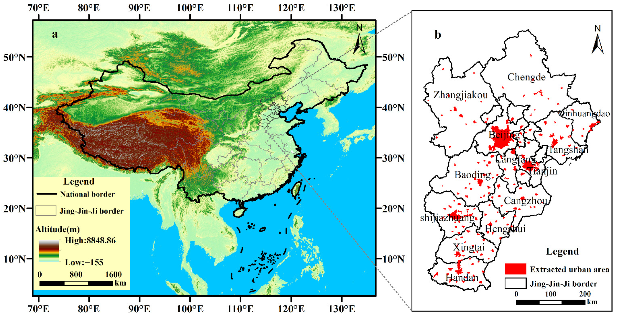
Figure 1. Study area in Beijing–Tianjin–Hebei. (Note that the location of Beijing-Tianjin-Hebei in China (a). The merging and screening of the urban boundary and non-urban land patches were based on the land use status in different periods according to the degree of patch continuity and the influence of the ocean or cities in other provinces; the continuous patches were therefore taken as a research unit, whereas those affected by sea water and inaccurate classification were deleted. This screening and merging process yielded a total of 156 urban areas (b), which are independent of each other and continuous in time, and are not affected by the ocean or adjacent patches).
Remotesensing 14 02880 g001
Figure 2. Spatial distribution of summer precipitation in different periods in the Beijing–Tianjin–Hebei region.
Remotesensing 14 02880 g002
Figure 3. Spatial distribution of winter precipitation in different periods in the Beijing–Tianjin–Hebei region.
Remotesensing 14 02880 g003
Figure 4. Spatial distribution of annual precipitation in different periods in the Beijing–Tianjin–Hebei region.
Remotesensing 14 02880 g004
Figure 5. Spatial distribution of precipitation changes in different seasons in the Beijing–Tianjin–Hebei region ((a), summer; (b), winter; (c), annual, units: mm).
Remotesensing 14 02880 g005
Figure 6. Variations in precipitation in the Beijing–Tianjin–Hebei urban agglomeration from 2000 to 2018 (a), summer; (b), winter; (c), annual; green or light green means decrease, blue or light blue means increase; units: mm).
Remotesensing 14 02880 g006
Figure 7. Results of the optimal full subset regression (a), summer; (b), winter; (c), annual; the red font on the right indicates that the model was the best model).
Remotesensing 14 02880 g007
Figure 8. Ranking of influencing factors by season.
Remotesensing 14 02880 g008
Table 1. Influencing factors on precipitation used in this study.
Category of VariableVariableMeaning of VariableData Sources
Urban form factorFRAC FRAC = 2 ln 0.25 p i j l n a i j ,
P i j = perimeter (m) of patch ij, a i j = area (m2) of patch ij. FRAC can help quantify the degree of complexity of the planar shapes.
Calculated from the 30 m land use data (https://www.resdc.cn/data.aspx?DATAID=283) (accessed on 1 September 2020)
CIRCLE CIRCLE = 1 a i j a i j s
a i j = area (m2) of grid ij. a i j s = area (m2) of smallest circumscribing circle around grid ij. CIRCLE is used to distinguish patches that are linear (narrow) or elongated
Calculated from the 30 m land use data (https://www.resdc.cn/data.aspx?DATAID=283) (accessed on 1 September 2020)
CONTIG CONTIG = p = 1 n c i j p a i j * 1 s 1
c i j r = contiguity value of pixel p in zone ij, a i j * = area of zone ij is represented by the number of grids, s = sum of the values in a 3-by-3 grid template. CONTIG assesses the spatial connectedness or contiguity of cells within a grid cell patch (equals 0 for a one-pixel patch and increases to a limit of 1 as patch contiguity or connectedness increases)
Calculated from the 30 m land use data (https://www.resdc.cn/data.aspx?DATAID=283) (accessed on 1 September 2020)
Urbanization development levelPOPRepresents the degree of population densityhttp://sedac.ciesin.columbia.edu/data/set/gpw-v4-population-density-rev10 (accessed on 1 September 2020)
NLIDenotes the light generated from electricity (areas of high economic prosperity and population are generally well-illuminated)Defense Meteorological Satellite
Program-Operational Linescan System (DMSP-OLS)
AREAIndicates the area of urban expansionBased on the 30 m land use data (https://www.resdc.cn/data.aspx?DATAID=283) (accessed on 20 September 2020)
Natural/meteorological conditionsRHUAverage relative humidity of an urban administrative unithttp://data.cma.cn/data/detail/dataCode/A.0012.0001.html (accessed on 20 September 2020)
WINAverage wind speed of an urban administrative unit (m/s)http://data.cma.cn/data/detail/dataCode/A.0012.0001.html (accessed on 20 September 2020)
RADAverage radiation of an urban administrative unithttp://data.cma.cn/data/cdcdetail/dataCode/RADI_MUL_CHN_DAY.html (accessed on 20 September 2020)
ALTAverage altitude of urban areas obtained from DEM (digital elevation model) data with a resolution of 30 m
Surface propertiesNDVINormalized transform of the NIR (near-infrared radiation) to red reflectance ratio (commonly designed to standardize vegetation indices values to between −1 and +1)https://lpdaac.usgs.gov/dataset_discovery/modis/modis_products_table/mod13a3_v006 (accessed on 1 September 2020)
TREEPercentage of urban forest coveragehttps://modis.gsfc.nasa.gov/data/dataprod/mod44.php (accessed on 1 September 2020)
Air qualityAODAerosol optical depth, the key physical quantity that characterizes the degree of atmospheric turbidityhttps://sedac.ciesin.columbia.edu/data/set/sdei-global-annual-gwr-pm2–5-modis-misr-seawifs-aod-v4-gl-03 (accessed on 1 September 2020)
PM2.5Particulate matter with a diameter of less than 2.5 microns can enter the lungs (expressed as fine particulate matter, in terms of the annual average concentration of micrograms per cubic meter)https://nasasearch.nasa.gov/search?query=PM2.5&affiliate=nasa&utf8=%E2%9C%93 (accessed on 20 September 2020)
Urban thermal environmentUHIAverage surface temperature of the inner city area minus the average surface temperature of the suburbs 10 km from the buffer zoneCalculated from LST data (http://www.gscloud.cn/sources/accessdata/336?pid=333) (accessed on 20 September 2020)
LSTAverage surface temperature of the inner city area http://www.gscloud.cn/sources/accessdata/336?pid=333 (accessed on 20 September 2020)
Table 2. Ordinary least squares (OLS) and stepwise regression results for factors affecting urban precipitation.
Category of VariableVariableSummerWinterAnnual
R2Adj R2R2Adj R2R2Adj R2
Urban form factorFRAC0.01 ** (+)0.010.002 (+/)/0.006 (−)0.05
CIRCLE0.01 ** (+/)0.003 (+/)0.001 (−/)
CONTIG0.000 (+/)0.000 (+/)0.004 (−/)
Urbanization development levelPOP0.000 (+/)0.1030.004 (−)0.0460.000 (−)0.075
NLI0.072 *** (+)0.017 ** (+)0.032 *** (−)
AREA0.007 * (+)0.000 (−/)0.036 *** (−)
Natural/meteorological conditionsRHU0.314 *** (+)0.3450.003 (−/)0.1590.060 *** (+)0.107
WIN0.003 (+)0.021 *** (−)0.000 (−/)
RAD0.012 *** (−)0.011 ** (+/)0.000 (+)
ALT0.000 (+)0.135 *** (+)0.025 *** (−)
Surface propertiesNDVI0.093 *** (+)0.1320.111 *** (−)0.1090.001 (−/)0.006
TREE0.000 (−)0.019 ** (−/)0.008 (+)
Air qualityAOD0.002 (−/)/0.128 *** (−)0.1480.014 ** (−)0.012
PM2.50.005 (−/)0.093 *** (−)0.003 (−/)
Urban thermal environmentUHI0.041 *** (+)0.1660.011 ** (−)0.2280.051 *** (−)0.062
LST0.140 *** (−)0.226 *** (−)0.008 * (+)
Note: ***, **, and * represent significance at the 0.001, 0.01, and 0.05 levels, respectively. The R2 column shows the OLS regression results for a factor analyzed alone with precipitation. (+) and (−) indicate that the correlation between the explanatory variable and precipitation is positive or negative, respectively. Adj R2 shows the result of stepwise regression between each factor layer and precipitation. The symbol/indicates that the variable did not enter the stepwise regression equation.
Publisher’s Note: MDPI stays neutral with regard to jurisdictional claims in published maps and institutional affiliations.