Article

Summer Marine Heatwaves in the Kuroshio-Oyashio Extension Region

1
CAS Key Laboratory of Ocean Circulation and Waves, Institute of Oceanology, Chinese Academy of Sciences, Qingdao 266071, China
2
University of Chinese Academy of Sciences, Beijing 100049, China
3
CSIRO Oceans and Atmosphere, Indian Ocean Marine Research Centre, Crawley, WA 6009, Australia
4
Centre for Southern Hemisphere Ocean Research, Hobart, TAS 7000, Australia
5
Pilot National Laboratory for Marine Science and Technology, Qingdao 266237, China
6
Center for Ocean Mega-Science, Chinese Academy of Sciences, Qingdao 266071, China
7
CAS Engineering Laboratory for Marine Ranching, Institute of Oceanology, Chinese Academy of Sciences, Qingdao 266071, China
8
CSIRO Oceans and Atmosphere, Hobart, TAS 7000, Australia
*
Author to whom correspondence should be addressed.
Remote Sens. 2022, 14(13), 2980; https://doi.org/10.3390/rs14132980
Submission received: 6 April 2022 / Revised: 3 May 2022 / Accepted: 18 June 2022 / Published: 22 June 2022

Abstract

:
During 1982–2021, the highest sea surface temperature (SST) variability over the North Pacific was in the Kuroshio-Oyashio Extension (KOE) region, with more intense marine heatwaves (MHWs), especially during summertime. In this study, we explored the evolution and driving factors of the strongest summer MHWs based on their cumulative intensity using satellite observations and reanalyzed model results. Strong summer MHWs in 1999, 2008, 2012, and 2016 were initiated and peaked around summer. The more recent summer MHW events in 2018, 2020, and 2021 appeared to be associated with intermittent MHW events in the previous winter that extended to boreal summer. Based on a mixed layer temperature budget analysis from March to their peaks in summer, MHWs in 1999, 2008, 2012, and 2016 were primarily driven by the air-sea heat flux anomalies, with anomalous shortwave radiation due to reduced cloud cover being the dominant factor. Summer MHWs in 2018, 2020, and 2021 were mainly contributed by the ocean memory of winter warming. The northward shift of the Kuroshio Extension axis, the northward intrusion of the anticyclonic eddies, and the decadal warming trend may contribute to the positive sea surface height anomalies and increased upper ocean heat content in the KOE to increase winter SST and precondition the summer MHWs. Understanding MHW variability and the underlying mechanisms will help manage the marine ecosystem of the KOE region, as well as predict climate change impacts.

1. Introduction

Extreme events in the ocean are becoming more frequent, causing severe ecological disasters and socio-economic losses [1,2,3]. Marine heatwaves (MHWs; [4]) are extreme thermal events with abnormally high sea surface temperature (SST) at a specific location during a certain period. They can extend over hundreds to thousands of kilometers and last for up to hundreds of days [5]. MHWs can be affected by atmospheric processes and ocean circulation processes (e.g., [6,7]). Notably, MHWs can lead to severe environmental and ecological impacts, such as decreased surface chlorophyll levels due to increased ocean stratification [8], range shift [9], mass mortality of marine species [10,11], and causing detrimental impacts on fisheries [12,13].
Many MHWs, with diverse physical drivers, have been recorded over the global ocean [5,6]. The five major West Boundary Currents (WBCs) and their extension regions, with large SST variability of 2~5 °C, are prominent MHW hotspots [6], such as MHWs off southeast Australia in 2015/16 [14,15], the Northwest Atlantic in 2012 and during 1993–2018 [16], and the Southwest Atlantic in 2017 [17]. Recently, MHWs in the Northwest Pacific have also attracted wide attention: Miyama et al. [18] explained that the MHWs in the Oyashio region during summer in 2010–2016 were attributed to increased anticyclonic eddy activity; Kuroda and Setou [19] reported that a MHW occurred in July-August 2021 over the Northwest Pacific, including the entire Sea of Japan and part of the Sea of Okhotsk, which was mainly caused by anomalous surface heat flux forced by the atmospheric conditions.
The Kuroshio-Oyashio Extension (KOE; 141–175°E, 35–44°N) region has the largest SST variability (Figure 1a) and the fastest long-term warming rate in the North Pacific [20,21]. Therefore, it is imperative to systematically detect and quantify the mechanism of MHWs in the KOE region. The KOE is located between the northern branch of the Kuroshio Extension (KE; 141–150°E, 35–40°N) front and the Oyashio subarctic front, with a large meridional SST gradient and vigorous air-sea heat exchanges [22,23]. The Kuroshio, the WBC of the North Pacific subtropical gyre, forms a swift eastward jet along the coast of Japan before leaving the Japan coast at ~35°N, carrying warm and saline waters northeastward and releasing large amounts of heat into the atmosphere [24,25]. The Oyashio is the WBC of the western subarctic gyre, branching off the Japan coast at ~41°N, of which part of the Oyashio water in the intermediate layer is fed into the subtropical gyre, and the rest returns to the western subarctic gyre [26]. The zone between the two extensions is important fishing ground. SST anomalies (SSTA) in this region greatly affect the population dynamics of Japanese sardines [27,28] and saury migration [29,30].
Previous research in the KOE and KE regions mainly focused on wintertime SST variability, with identified driving factors including El Niño-Southern Oscillation (ENSO)-driven atmospheric circulation disturbances [31], KE path migration [32,33], and mixed layer depth (MLD) variation [34,35]. The KOE region has the highest SST variability in the Northwest Pacific (Figure 1a), especially in summer (Figure 1b), with the potential for strong MHWs. In this study, we examined SST and MHW variability in the KOE region, with a focus on the summer season, aiming to analyze their evolution, quantify their driving factors, and assess the influences from atmospheric circulation systems and ocean circulation. This paper is organized as follows. Section 2 describes the materials and methods; In Section 3, we detect MHWs in the KOE region during 1982–2021, and analyze their forcing mechanisms; Section 4 and Section 5 provide discussion and conclusions.

2. Materials and Methods

2.1. Materials

2.1.1. Satellite Observation Data

The datasets and key components used in this study are listed in Table 1. The National Oceanic and Atmospheric Administration Optimum Interpolated Sea Surface Temperature (NOAA OISST) Version 2 [36] is based upon the Advanced Very High-Resolution Radiometer (AVHRR) satellite, with daily and monthly resolution. The Ssalto/Ducas daily sea surface height (SSH) and geostrophic current (u, v) products on the Copernicus Marine Environment Monitoring Service (CMEMS) website are used, including the delayed time data from 1993 to 2020 and near-real time data from 2021 [37]. The monthly outgoing longwave radiation (OLR) data from NOAA polar-orbiting satellites [38] and the monthly precipitation (PRE) data from Climate Prediction Center (CPC) Merged Analysis of Precipitation (CMAP) [39] are also used.

2.1.2. Reanalysis Data

For the ocean, we used data from the National Centers for Environmental Prediction (NCEP) Global Ocean Data Analysis System (GODAS) [40]. This product is based on a quasi-global configuration of the Geophysical Fluid Dynamics Laboratory Modular Ocean Model version 3, assimilating data from expendable bathythermographs (XBTs), Tropical Atmosphere Ocean (TAO), Triangle Trans-Ocean Buoy Network (TRITON), Prediction and Research Moored Array in the Tropical Atlantic (PIRATA), and Argo profiling floats. Data used in the study include potential temperature (T), zonal and meridional components of horizontal current (u, v), geometric vertical velocity (w), air-sea heat flux, and MLD. For atmospheric variables, data from the National Centers for Environmental Prediction (NCEP) Climate Forecast System Reanalysis (CFSR) [41] and Climate Forecast System version 2 (CFSv2) [42] were used, including monthly sea level pressure (SLP), total cloud cover (TCC), and daily air-sea heat flux (shortwave radiation, longwave radiation, sensible heat flux, latent heat flux).

2.2. MHW Definition

The definition of MHW was following Hobday et al. [4], as a discrete prolonged anomalously warm water event when the daily SST exceeds a 90th percentile threshold based on a long-term climatology for five or more days. The 90th percentile threshold and climatological mean were calculated for each calendar day from daily SST within an 11-day window and a 31-day moving average. MHWs with gaps of less than two days were considered a continuous event. In this study, the threshold and climatology were determined over a base period of 1982–2021 from NOAA OISST. Here, we describe MHW characteristics by a series of metrics, including mean intensity (the average temperature anomaly above the threshold over the duration of an event), days (the total number of MHW days in each year or season), and cumulative intensity (the integrated intensity over the duration of the event) [4,14].

2.3. Model Verification

Before analyzing the mixed layer (ML) heat budget, we assessed the accuracy of GODAS temperature data with satellite observation. The Root Mean Square Error (RMSE) of summer daily SST between GODAS and OISST was mostly less than 1 °C, except near the Japan coast (Figure 2a), with correlation coefficient (CC) mostly above 0.8 and reaching ~0.9 in eastern KOE (Figure 2b). Averaged in the KOE region, summer SSTA from the two products were well correlated, with a correlation of 0.97 (Figure 2c). Thus, the GODAS SST can realistically reproduce satellite SST variability in this region. Note that GODAS doesn’t assimilate satellite SST data, which may have caused small differences between the two in some of the recent years.

2.4. Mixed Layer Heat Budget

To quantitatively assess the SST warming during the MHWs, we performed a heat budget analysis of the ocean ML temperature [43,44,45]. Averaged within a control area A in the KOE domain (Figure 1a, box), the ML temperature equation can be written as:
1 A A T m t d A = 1 A A U m · T m d A + 1 ρ C P A A Q n e t h m d A 1 A A w e Δ T h m d A + R e s
where T m is the ML temperature, representing summer SST; h m is the MLD; U m is the horizontal velocity vertically averaged in the ML, including the zonal (u) and meridional (v) components, and ∇ denotes the gradient operator in the two directions; ρ and C P are the reference density (1024 kg m−3) and heat capacity of seawater (3985 J kg−1 °C−1), respectively; Q n e t is net air-sea heat flux; w e is entrainment velocity. In the following, we refer to the terms in Equation (1) as temperature tendency (left, T T o t a l ), and the contribution of the horizontal advection ( T A d v ), surface net heat flux ( T Q n e t ), vertical entrainment ( T V E ), and residual ( T R e s ). In particular, the MLD is provided in the GODAS output, which is estimated as a depth where the density difference relative to the surface level is 0.03 kg m−3 [40,46]. In summer, the lowest MLD is limited to 20 m. Δ T = T m T d , which is the temperature difference between ML temperature ( T m ) and at 10 m below the ML base ( T d ) [47].
The net air-sea heat flux is decomposed as:
Q n e t = Q s w + Q l w + Q s h f + Q l h f = q ( 0 ) q ( - h ) + Q l w + Q s h f + Q l h f
where Q s w is the shortwave radiation absorbed in the ML, and Q l w , Q s h f , Q l h f are the surface net longwave radiation, sensible heat flux, and latent heat flux, respectively. Moreover, q ( 0 ) is the surface download shortwave radiative flux, and q ( - h ) represents the penetrating shortwave radiation [48]. In the remainder of this paper, we express the surface heat flux into (out of) the ocean as a positive (negative) heat flux.

3. Results

3.1. MHWs in the KOE during 1982–2021

The frequency of MHWs in the KOE region showed a prominent increase over the past four decades, especially in the last decade, which was closely related to the observed long-term warming trend (Figure 3a; [49,50]). The mean intensity and cumulative intensity of MHW showed noticeable seasonal variations, with weaker seasonal variations in the total MHW days (Figure 3b,d,f). Particularly, the cumulative intensity of MHW, which combines the effects of mean intensity and duration, is a good proxy for the potential impact of MHW on marine ecosystems [51]. The cumulative intensity of MHWs in the KOE region was highest in summer, almost twice as those in spring or winter (Figure 3f), consistent with strong summer SSTA variability (Figure 1b).
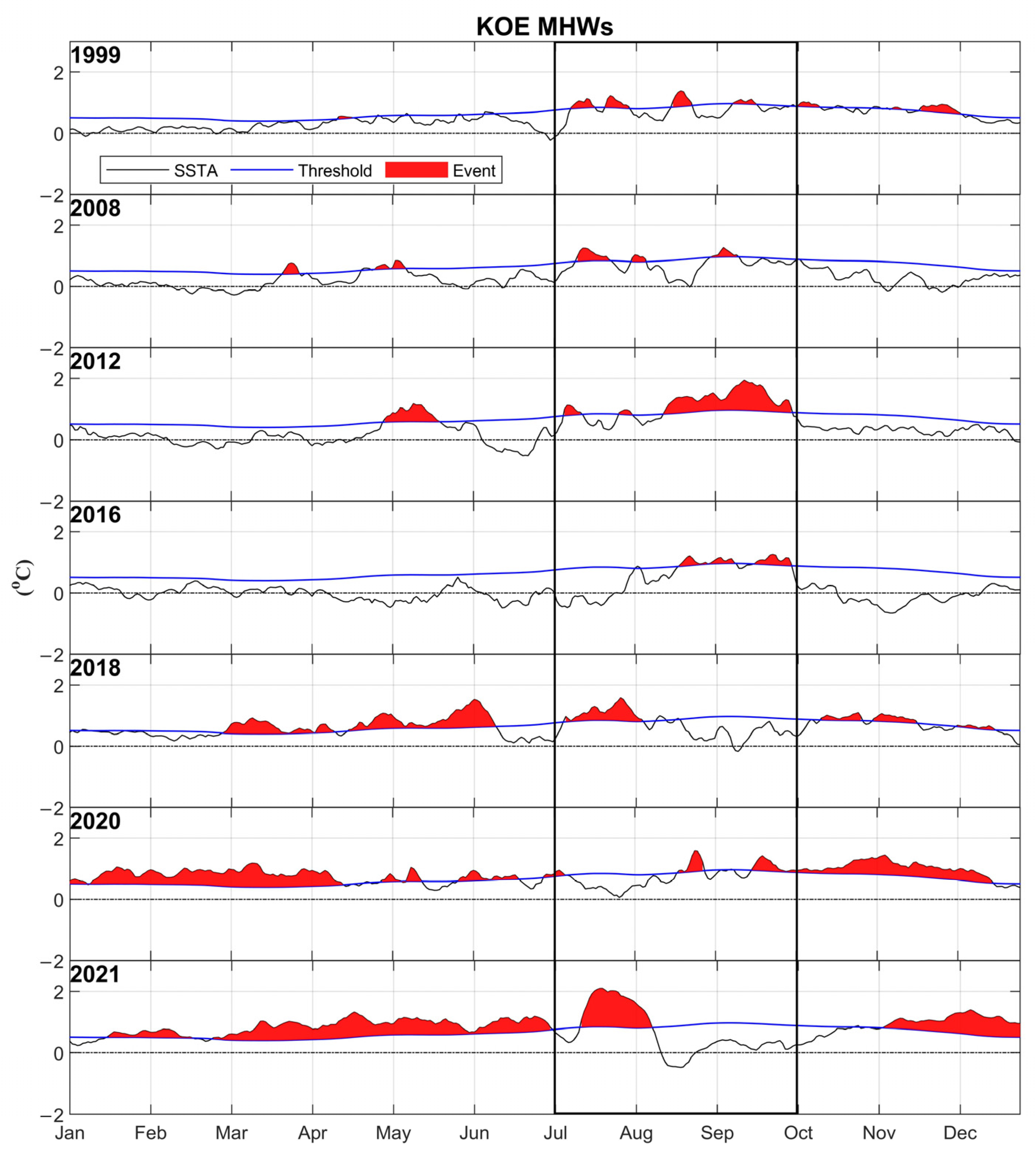
Focusing on the summer MHWs in the KOE region, the seven strongest events were selected based on the summer averaged cumulative intensity exceeding 30 °C day (Figure 3g). The MHWs in 1999, 2008, 2012, and 2016 were mainly initiated and peaked in summer, with some smaller intermittent MHWs in other seasons (Figure 4). However, the MHWs in 2018, 2020, and 2021 already existed in the previous winter (particularly in March), and the warm anomalies continued to develop in spring and peaked in summertime (Figure 4). Other stronger summer MHW events, such as 1998, 2010, 2011, and 2013 will be briefly described in Appendix A.

3.2. Mechanisms of MHWs

In this section, we used the ML heat budget analysis to understand the driving mechanisms of the strongest MHWs in JAS.

3.2.1. Heat Budget Analysis

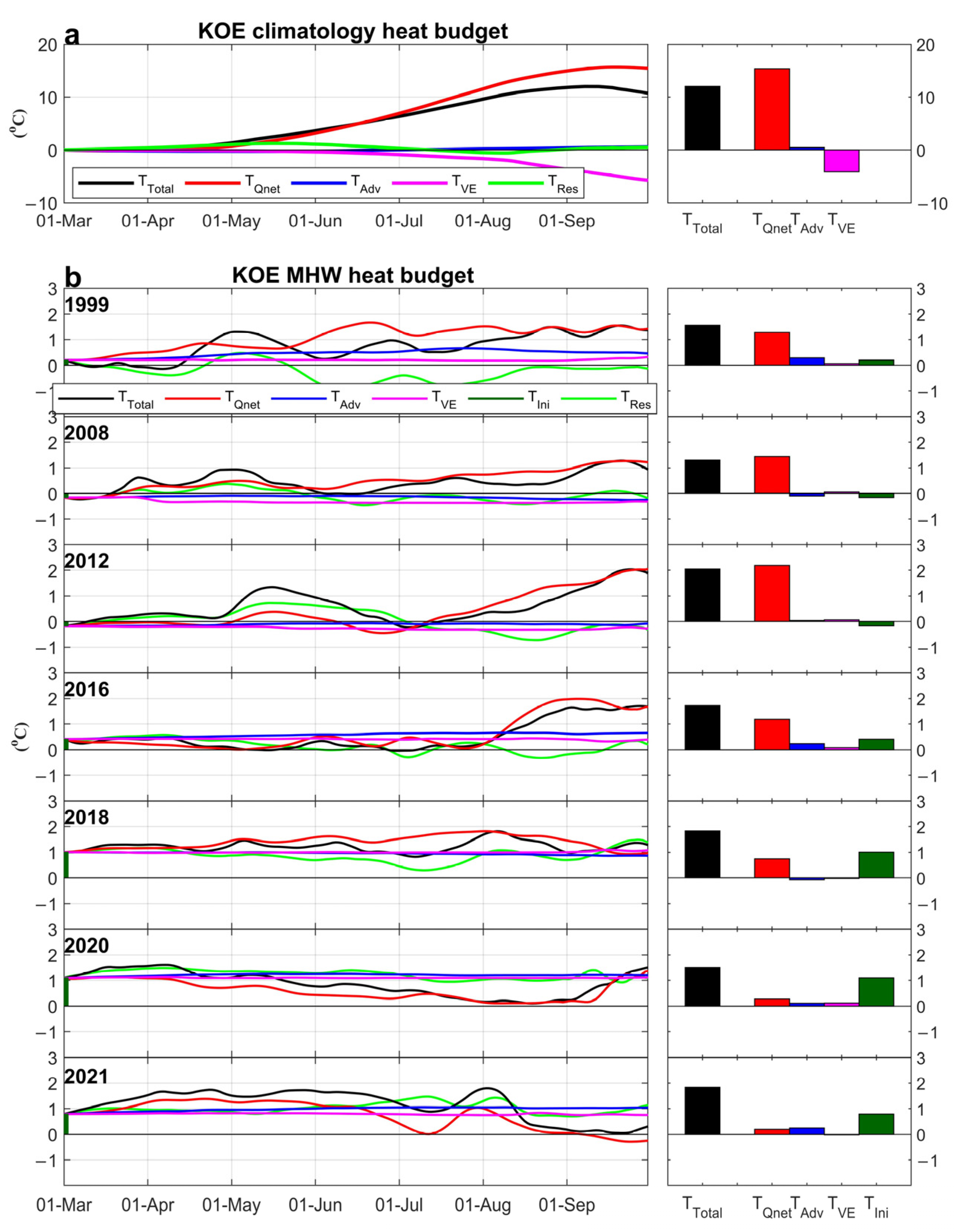
To quantitatively evaluate the driving mechanisms of the seven strongest MHWs in the KOE region, we examined the daily ML temperature budget from March to September (Figure 5), which covers the seasonal warming period. The climatology ML temperature reaches a peak in early-September. The seasonal warming is mainly controlled by the net air-sea heat flux, with little contribution from advection. Notably, entrainment cooling becomes increasingly important in summer, partly balancing the surface heat flux contribution (Figure 5a; [34]).
Peak temperature anomalies of summer MHWs in 1999, 2008, 2012, and 2016 were mainly contributed by air-sea heat flux anomalies (1.3 °C, 1.4 °C, 2.2 °C and 1.2 °C, respectively; Figure 5b). In 2018, 2020, and 2021, however, significant warming had already existed at the end of previous winters (1 March), at 1.0 °C, 1.1 °C, and 0.8 °C, respectively. Contributions from anomalous air-sea heat fluxes were less significant (Figure 5b). Thus, the summer MHW peaks in the early events were mainly caused by anomalous air-sea heat flux, whereas in 2018, 2020, and 2021, ocean memory of winter warming was the key factor.

3.2.2. The Effect of Air-Sea Heat Flux

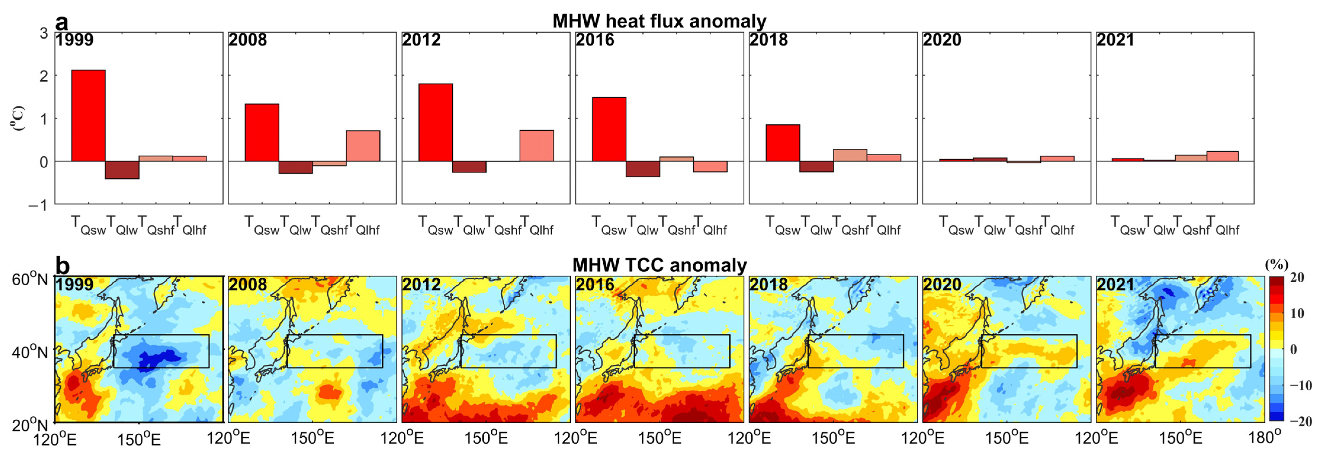
The summer MHWs in 1999, 2008, 2012, and 2016 were mainly caused by air-sea heat flux anomalies (Figure 5b). Based on NCEP CFSR/CFSv2 atmospheric reanalysis products, shortwave radiation flux anomalies were the leading component in causing the peak ML temperature anomalies among the surface heat flux terms in 1999, 2008, 2012, 2016, and 2018 (Figure 6a). Consequently, shortwave radiation anomalies were the major driving force of the summer MHWs in 1999, 2008, 2012, 2016. Other flux terms played a lesser role in the MHW development. In 2018, the shortwave radiation contribution was only secondary to winter warming in causing the summer MHW (Figure 5b).
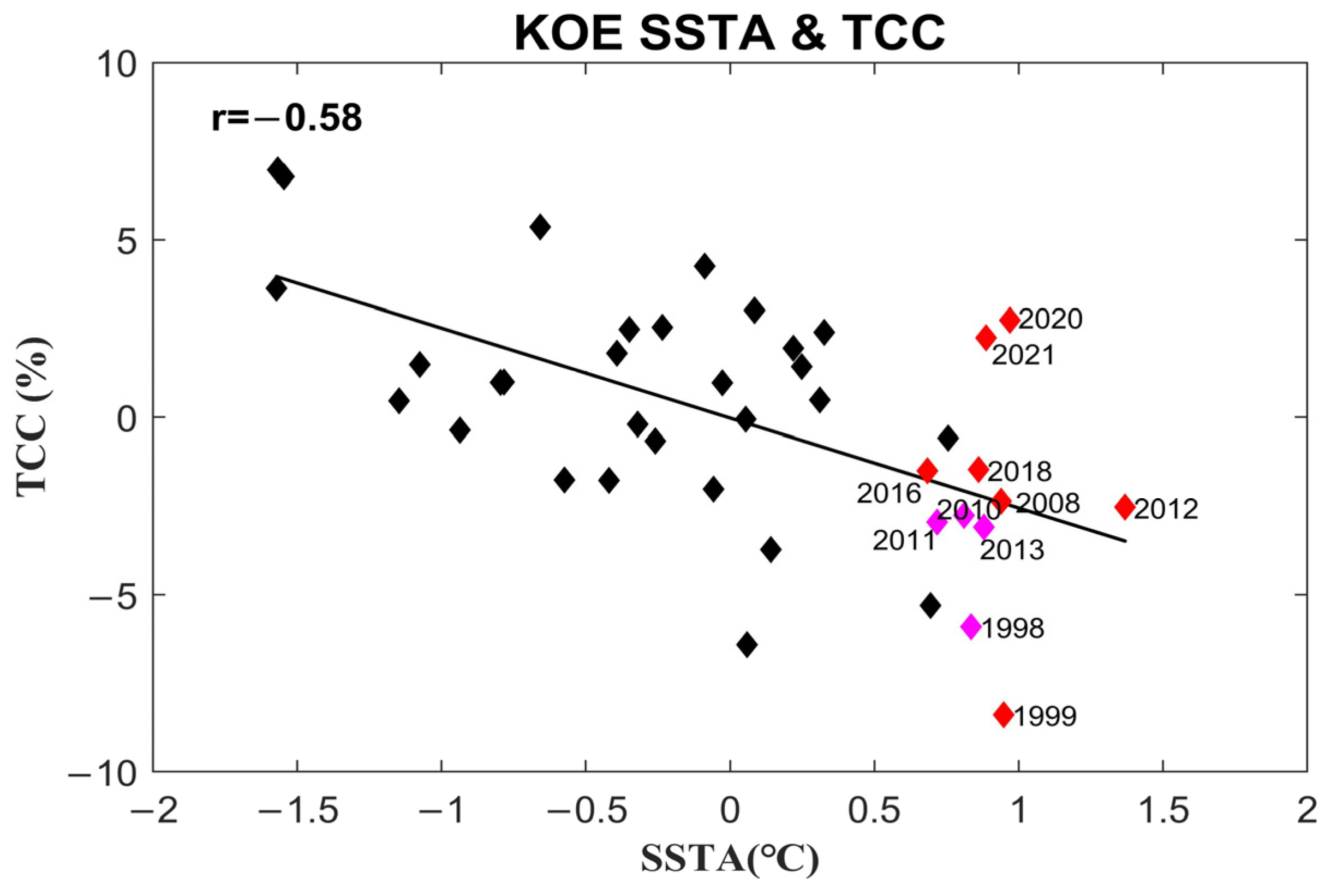
During summertime, the air-sea feedback between cloud cover and SST was particularly significant [46,52]. Reduced TCC in the KOE region corresponded well with the increased shortwave radiation anomalies that dominated in the summer MHW development (Figure 6b). Furthermore, the anti-correlation between TCC and SSTA in the KOE region reflected the shortwave radiation contribution to the MHWs in the region (Figure A2).

3.2.3. The Effect of Winter Warming

Summer MHWs in 2018, 2020, and 2021 developed upon abnormally large ML temperature warming at the end of winter (1 March) (Figure 5b).To explore the effect of the winter ocean warming, we examined the wintertime SSH variability and upper ocean temperature anomalies during the MHW years (Figure 7). On average, the Kuroshio separates from the coast at 35°N and extends eastward following two quasi-stationary meanders with a strong SSH gradient (Figure 1a,c). There were positive SSH anomalies in the KOE region in 2018, 2020, and 2021, with enhanced anticyclonic eddy activities (Figure 7). In 2020 and 2021, there were significant positive SSH anomalies near the southern boundary of the KOE region, indicating a northward migration of the KE axis (Figure 7a). In addition, there was a strong SSH trend in the KOE region after 2018, indicating heat accumulation in the KOE region (Figure 8).
Furthermore, the vertical profile of temperature anomalies in the KOE showed that there was higher winter warming of the upper ocean in 2018, 2020, and 2021 (Figure 7b). As winter warming persisted into spring and summer, they would have preconditioned the MHWs in summer.

4. Discussion

4.1. Impact of Atmospheric Circulation System

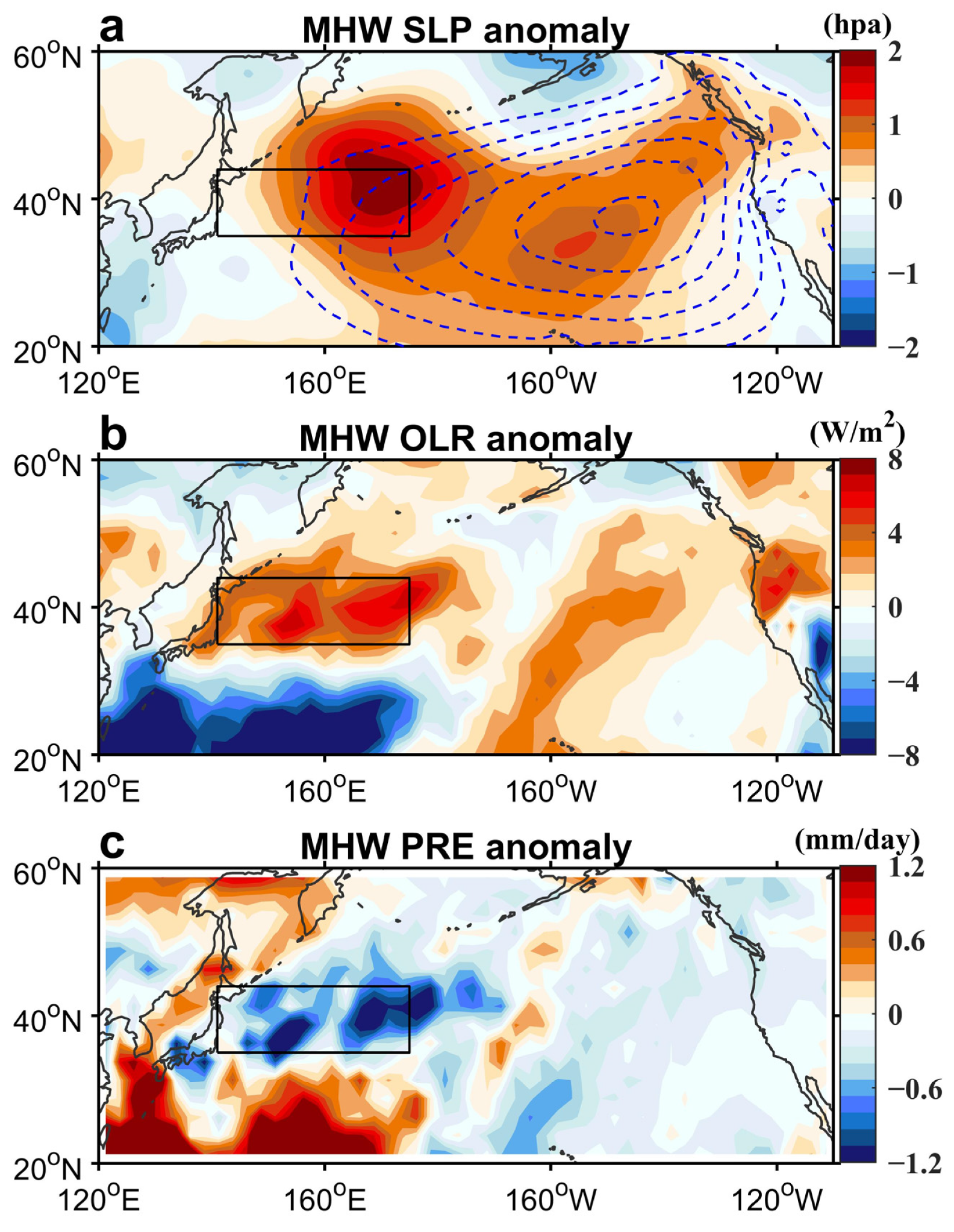
Strong summer MHWs in 1999, 2008, 2012, and 2016 in the KOE region, the positive shortwave radiation anomalies were prominent during summertime, associated with the reduction in cloud cover (Figure 6). Further analysis found that the reduction of cloud cover in the KOE was primarily explained by the anomalously strengthened North Pacific High (NPH) system (Figure 9a), which suppressed the convective activity, manifested as positive OLR and negative precipitation anomalies (Figure 9b,c). Similarly, Kuroda and Setou [19] found that MHW in the Northwest Pacific in summer 2021 was related to air-sea heat fluxes, and the northwestern shift of the NPH was an important factor. However, besides the NPH system, some other factors were still worthy of consideration. For example, the northward movement of the westerly jet induced warm atmospheric conditions [19]; the Philippine-Japan teleconnection triggered by the SST-forced tropical Pacific anomaly led to the great decay of cloud amounts near Japan [53]. All these factors can have some effect on the KOE region, resulting in an anomalous increase in SST. The large-scale drivers of atmospheric circulation systems in the KOE region are worth further attention.

4.2. Factors Affecting Upper Ocean Heat Content

The winter memory dominated MHWs (2018, 2020, and 2021) were closely associated with the upper ocean heat content in the KOE region (Figure 7). Previous studies demonstrated that the KE index represents the low-frequency variability of the KE system [33,54]. For example, KE had significant decadal variability between stable and unstable dynamic states [32,33,54]. Specifically, the stable state exhibited a northward shift of KE and an intensified recirculation gyre [54], with a significant decadal warming trend since 2018 (Figure 8), which is consistent with the increasing occurrences of MHWs in the KOE region. The decadal modulation of the KE system was related to the basin-scale wind stress associated with the Pacific Decadal Oscillation (PDO) [55], and the negative PDO phase can lead the positive SSH anomalies by three years [54]. Influences from the ocean dynamic processes on the KOE warming or cooling events, such as Rossby waves and North Pacific oscillations, need to be further studied.
Another factor worth considering forced the northward shift of the KE axis was the long-term global warming. The enhanced warming trend showed a synchronous change with the subtropical WBCs. Wu et al. [20] proposed that the Kuroshio Current has shifted poleward by about 0.8 ± 0.4° in the past century, which was associated with a regional warming trend. Yang et al. [21] pointed out that the Kuroshio Current would strengthen and shift poleward under global warming. In general, the northward migration of the KE axis in recent years may be due to the superposition of internal decadal oscillations and externally forced warming trends.

4.3. Biological Implications

MHWs in a region can cause stress for marine life. Mobile or migratory species may move elsewhere, or deeper, to remain in their preferred temperature range. For lower mobility species (or life stages), or where MHW conditions are spatially extensive, declines in survival or performance have been reported from around the world [56]. Long-term changes in the distribution of coastal species adjacent to the Kuroshio have been reported (e.g., [57]), but less is known in the more offshore KOE region. This region is an important foraging ground for a range of marine species, including marine mammals (e.g., [58]), presumably exploiting the rich feeding environment created by the convergence of the warm and cold currents. In turn, offshore fisheries have also used this region for many decades, and have long noted the relationship between SST and the abundance of the focal species, particularly saury [59]. With the predicted increase in the frequency, duration, and intensity of MHWs, an understanding of species responses to extremes can help anticipate and plan responses to offset unwanted outcomes for species and fisheries.

5. Conclusions

As the region with the largest SST variability in the North Pacific, the KOE has been experiencing more intense MHWs over the past four decades. Particularly, the cumulative intensity during boreal summer was the strongest, almost twice that of spring or winter. In this study, we explored the summer MHWs in the KOE region and analyzed the seven strongest summer MHWs based on cumulative intensities. We found that the MHWs in 1999, 2008, 2012, and 2016 mainly initiated and reached their peak temperature in summer, while in 2018, 2020, and 2021, MHWs in winter persisted, some intermittently, and continued to affect boreal summer. ML temperature budget analysis showed that MHWs in 1999, 2008, 2012, and 2016 were mainly driven by the air-sea heat flux due to the increased shortwave radiation associated with the reduced cloud cover; MHWs in 2018, 2020, and 2021 were primarily contributed by the initial value of winter ML which was associated with the anomalous KE axial migration and the decadal warming trend to produce positive upper ocean heat content anomalies. A better understanding of the driving mechanism of MHWs in the KOE region provides a reference for projecting MHWs in the region in future climate change.

Author Contributions

Conceptualization, Y.D., M.F. and Z.X.; methodology, Y.D., M.F., Z.X. and B.Y.; writing-original draft presentation, Y.D.; writing-review and editing, M.F., Z.X. and A.J.H. All authors have read and agreed to the published version of the manuscript.

Funding

This study was jointly supported by the National Natural Science Foundation of China (NSFC), the Strategic Pioneering Research Program of CAS, the NSFC-Shandong Joint Fund, the National Key Research and Development Program of China (92058202, XDB42000000, XDA22050202, 42076022, U1806227, 2017YFA0604102), the CAS Key Research Program of Frontier Sciences, the Key Deployment Project of Center for Ocean Mega-Research of Science, and the project jointly funded by the CAS and CSIRO (QYZDB-SSW-DQC024, COMS2020Q07, 133244KYSB20190031), Shandong special funding for Qingdao Pilot National Laboratory for Marine Science and Technology (No.2022QNLM010302).

Data Availability Statement

NOAA OISST provided by the NOAA/OAR/ESRL PSD, Boulder, Colorado, USA, from their web site at https://psl.noaa.gov/data/gridded/data.noaa.oisst.v2.highres.html (accessed on 17 June 2022). The altimetry sea surface height and geostrophic current data used are obtained from the Copernicus Marine Environment Monitoring Service (CMEMS), including the delayed time (SEALEVEL_GLO_PHY_CLIMATE_L4_MY_008_057) via (DOI) https://doi.org/10.48670/moi-00145 (accessed on 17 June 2022) and near-real time (SEALEVEL_GLO_PHY_L4_NRT_OBSERVATIONS_008_046) via (DOI) https://doi.org/10.48670/moi-00149 (accessed on 17 June 2022). NOAA OLR and CPC Merged Analysis of Precipitation data are obtained from https://psl.noaa.gov/data/gridded/data.olrdcdr.interp.html and https://climatedataguide.ucar.edu/climate-data/cmap-cpc-merged-analysis-precipitation (accessed on 17 June 2022). The GODAS data via https://psl.noaa.gov/data/gridded/data.godas.html (accessed on 17 June 2022). The CFSR/CFSv2 reanalysis data developed by National Centers for Environmental Prediction (NCEP), from their web site at https://hycom.org/dataserver/ncep-cfsr (accessed on 17 June 2022).

Acknowledgments

Thanks to Maxime Marin for the help in this work. This research is partly supported by the Centre for Southern Hemisphere Oceans Research (CSHOR), which is a joint initiative between the Qingdao National Laboratory for Marine Science and Technology (QNLM), CSIRO, University of New South Wales and University of Tasmania. We thank the anonymous reviewers for commenting on the early draft of the paper.

Conflicts of Interest

The authors declare no conflict of interest. The funders had no role in the design of the study; in the collection, analyses, or interpretation of data; in the writing of the manuscript, or in the decision to publish the results.

Appendix A

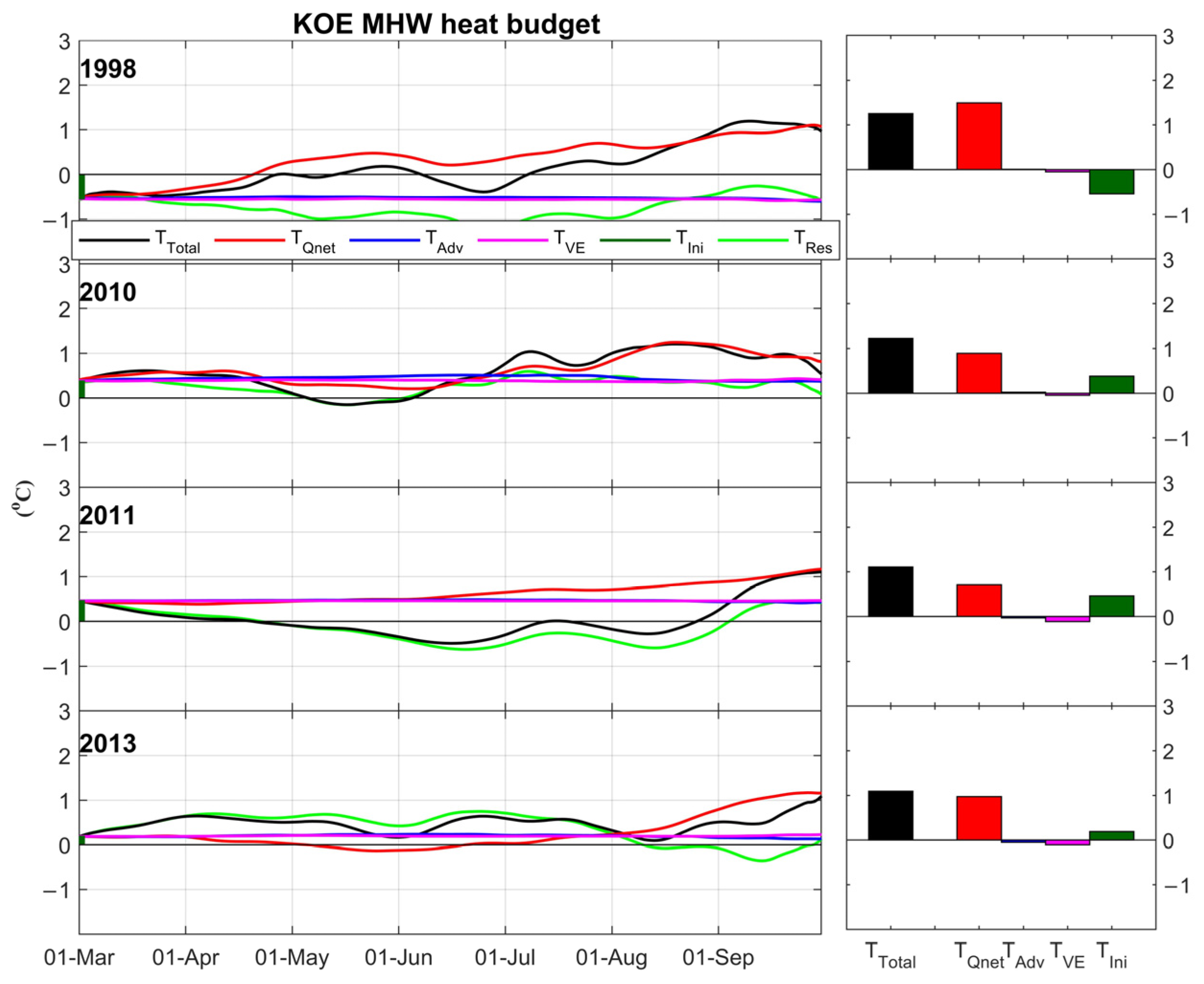
To further investigate the drivers of some of the less strong MHW events in the KOE region, the ML temperature budget analysis was calculated and shown in Figure A1. We found that the summer MHWs in 1998 and 2013 were mostly attributed to air-sea heat flux anomalies, whereas the summer MHWs in 2010 and 2011 were due to a mixed contribution from winter memory and air-sea heat flux anomalies.
Figure A1. ML temperature anomaly budget of the MHW years. Contributions from different terms to the temperature change from March to the summer peak values are shown in the right panels. Initial value contributions are denoted with dark green bars. The units of the right panels are the same as the left panels.
Remotesensing 14 02980 g0a1

Appendix B

To better clarify the driving role of TCC in severe SST/MHW, we further investigated the relationship between TCC and SSTA in the KOE region. As shown in Figure A2, lower TCC corresponded to stronger SSTA, with a correlation coefficient of −0.58.
Figure A2. Scatter diagram of the JAS averaged TCC and SSTA in the KOE region. The solid line denotes the linear regression. Red dots indicate the six largest MHWs and magenta dots indicate the less strong MHWs.
Remotesensing 14 02980 g0a2

Appendix C

Table A1. List of English Abbreviations.
AbbreviationFull name
AVHRRAdvanced Very High-Resolution Radiometer
AVISOArchiving, Validation, and Interpolation of Satellite Oceanographic
CCCorrelation Coefficient
CMEMSCopernicus Marine Environment Monitoring Service
CPC CMAPClimate Prediction Center Merged Analysis of Precipitation
ENSOEl Niño-Southern Oscillation
GODASGlobal Ocean Data Analysis System
KEKuroshio Extension
KOEKuroshio-Oyashio Extension
MHWMarine heatwave
ML/MLDMixed layer/Mixed layer depth
NCEP CFSR/CFSv2National Centers for Environmental Prediction Climate Forecast System Reanalysis and Climate Forecast System version 2
NOAA OI SSTNational Oceanic and Atmospheric Administration Optimum Interpolated Sea Surface Temperature
NPHNorth Pacific High
OLROutgoing longwave radiation
PIRATAPrediction and Research Moored Array in the Tropical Atlantic
PREPrecipitation
RMSERoot Mean Square Error
SLPSea level pressure
SSHSea surface height
SSTSea surface temperature
SSTASea surface temperature anomaly
TTemperature
TAOTropical Atmosphere Ocean
TCCTotal cloud cover
TRITONTriangle Trans-Ocean Buoy Network
WBCsWest Boundary Currents
XBTsExpendable bathythermographs

References

  1. Meehl, G.A.; Tebaldi, C. More intense, more frequent, and longer lasting heat waves in the 21st century. Science 2004, 305, 994–997. [Google Scholar] [CrossRef] [PubMed] [Green Version]
  2. Sun, J.Q.; Yuan, W.; Gao, Y.Z. Arabian Peninsula-North Pacific Oscillation and its association with the Asian summer monsoon. Sci. China Ser. D. Earth Sci. 2008, 51, 1001–1012. [Google Scholar] [CrossRef]
  3. Frölicher, T.L.; Fischer, E.M.; Gruber, N. Marine heatwaves under global warming. Nature 2018, 560, 360–364. [Google Scholar] [CrossRef]
  4. Hobday, A.J.; Alexander, L.V.; Perkins, S.E.; Smale, D.A.; Straub, S.C.; Oliver, E.C.J.; Benthuysen, J.A.; Burrows, M.T.; Donat, M.G.; Feng, M. A hierarchical approach to defining marine heatwaves. Prog. Oceanogr. 2016, 141, 227–238. [Google Scholar] [CrossRef] [Green Version]
  5. Sen Gupta, A.; Thomsen, M.; Benthuysen, J.A.; Hobday, A.J.; Smale, D.A. Drivers and impacts of the most extreme marine heatwaves events. Sci. Rep. 2020, 10, 19359. [Google Scholar] [CrossRef] [PubMed]
  6. Holbrook, N.J.; Scannell, H.A.; Gupta, A.S.; Benthuysen, J.A.; Feng, M.; Oliver, E.C.J.; Alexander, L.V.; Burrows, M.T.; Donat, M.G.; Hobday, A.J. A global assessment of marine heatwaves and their drivers. Nat. Commun. 2019, 10, 2624. [Google Scholar] [CrossRef]
  7. Gao, G.; Marin, M.; Feng, M.; Yin, B.; Yang, D.; Feng, X.; Ding, Y.; Song, D. Drivers of Marine Heatwaves in the East China Sea and the South Yellow Sea in Three Consecutive Summers During 2016–2018. J. Geophys. Res. Ocean. 2020, 125. [Google Scholar] [CrossRef]
  8. Bond, N.A.; Cronin, M.F.; Freeland, H.; Mantua, N. Causes and impacts of the 2014 warm anomaly in the NE Pacific. Geophys. Res. Lett. 2015, 42, 3414–3420. [Google Scholar] [CrossRef]
  9. Wernberg, T.; Bennett, S.; Babcock, R.C.; De Bettignies, T.; Cure, K.; Depczynski, M.; Dufois, F.; Fromont, J.; Fulton, C.J.; Hovey, R.K. Climate-driven regime shift of a temperate marine ecosystem. Science 2016, 353, 169–172. [Google Scholar] [CrossRef] [Green Version]
  10. Garrabou, J.; Coma, R.; Bensoussan, N.; Bally, M.; Cerrano, C. Mass mortality in Northwestern Mediterranean rocky benthic communities: Effects of the 2003 heat wave. Glob. Chang. Biol. 2010, 15, 1090–1103. [Google Scholar] [CrossRef]
  11. Genin, A.; Levy, L.; Sharon, G.; Raitsos, D.E.; Diamant, A. Rapid onsets of warming events trigger mass mortality of coral reef fish. Proc. Natl. Acad. Sci. USA 2020, 117, 25378–25385. [Google Scholar] [CrossRef] [PubMed]
  12. Caputi, N.; Kangas, M.; Chandrapavan, A.; Hart, A.; Lestang, S.D. Factors Affecting the Recovery of Invertebrate Stocks From the 2011 Western Australian Extreme Marine Heatwave. Front. Mar. Sci. 2019, 6, 484. [Google Scholar] [CrossRef] [Green Version]
  13. Barbeaux, S.J.; Holsman, K.; Zador, S. Marine Heatwave Stress Test of Ecosystem-Based Fisheries Management in the Gulf of Alaska Pacific Cod Fishery. Front. Mar. Sci. 2020, 7, 703. [Google Scholar] [CrossRef]
  14. Oliver, E.C.J.; Benthuysen, J.A.; Bindoff, N.L.; Hobday, A.J.; Holbrook, N.J.; Mundy, C.N.; Perkins-Kirkpatrick, S.E. The unprecedented 2015/16 Tasman Sea marine heatwave. Nat. Commun. 2017, 8, 16101. [Google Scholar] [CrossRef] [PubMed] [Green Version]
  15. Oliver, E.C.J.; Lago, V.; Hobday, A.J.; Holbrook, N.J.; Ling, S.D.; Mundy, C.N. Marine heatwaves off eastern Tasmania: Trends, interannual variability, and predictability. Prog. Oceanogr. 2018, 161, 116–130. [Google Scholar] [CrossRef]
  16. Scannell, H.A.; Pershing, A.J.; Alexander, M.A.; Thomas, A.C.; Mills, K.E. Frequency of marine heatwaves in the North Atlantic and North Pacific since 1950. Geophys. Res. Lett. 2016, 43, 2069–2076. [Google Scholar] [CrossRef] [Green Version]
  17. Manta, G.; Mello, S.D.; Trinchin, R.; Badagian, J.; Barreiro, M. The 2017 Record Marine Heatwave in the Southwestern Atlantic Shelf. Geophys. Res. Lett. 2018, 45, 12449–12456. [Google Scholar] [CrossRef]
  18. Miyama, T.; Minobe, S.; Goto, H. Marine Heatwave of Sea Surface Temperature of the Oyashio Region in Summer in 2010–2016. Front. Mar. Sci. 2021, 7, 576240. [Google Scholar] [CrossRef]
  19. Kuroda, H.; Setou, T. Extensive Marine Heatwaves at the Sea Surface in the Northwestern Pacific Ocean in Summer 2021. Remote Sens. 2021, 13, 3989. [Google Scholar] [CrossRef]
  20. Wu, L.; Cai, W.; Zhang, L.; Nakamura, H.; Timmermann, A.; Joyce, T.M.; Mcphaden, M.J.; Alexander, M.A.; Qiu, B.; Visbeck, M. Enhanced Warming over the Global Subtropical Western Boundary Currents. Nat. Clim. Chang. 2012, 2, 161–166. [Google Scholar] [CrossRef]
  21. Yang, H.; Lohmann, G.; Wei, W.; Dima, M.; Ionita, M.; Liu, J. Intensification and poleward shift of subtropical western boundary currents in a warming climate. J. Geophys. Res. 2016, 121, 4928–4945. [Google Scholar] [CrossRef] [Green Version]
  22. Yasuda, I. Hydrographic Structure and Variability in the Kuroshio-Oyashio Transition Area. J. Oceanogr. 2003, 59, 389–402. [Google Scholar] [CrossRef]
  23. Kwon, Y.O.; Alexander, M.A.; Bond, N.A.; Frankignoul, C.; Thompson, L.A. Role of the Gulf Stream and Kuroshio–Oyashio Systems in Large-Scale Atmosphere–Ocean Interaction: A Review. J. Clim. 2010, 23, 3249–3281. [Google Scholar] [CrossRef]
  24. Taguchi, B.; Xie, S.P.; Schneider, N.; Nonaka, M.; Sasaki, H.; Sasai, Y. Decadal Variability of the Kuroshio Extension: Observations and an Eddy-Resolving Model Hindcast. J. Clim. 2007, 20, 2357–2377. [Google Scholar] [CrossRef] [Green Version]
  25. Xu, Z.; Wang, Y.; Liu, Z.; McWilliams, J.C.; Gan, J. Insight into the Dynamics of the Radiating Internal Tide Associated with the Kuroshio Current. J. Geophys. Res. Ocean. 2021, 126, e2020JC017018. [Google Scholar] [CrossRef]
  26. Yasuda, I. North Pacific Intermediate Water: Progress in SAGE (SubArctic Gyre Experiment) and Related Projects. J. Oceanogr. 2004, 60, 385–395. [Google Scholar] [CrossRef]
  27. Noto, M. Population decline of the Japanese sardine, Sardinops melanostictus, in relation to sea surface temperature in the Kuroshio Extension. Can. J. Fish. 1999, 56, 973–983. [Google Scholar] [CrossRef]
  28. Noto, M.; Yasuda, I. Empirical biomass model for the Japanese sardine, Sardinops melanostictus, with sea surface temperature in the Kuroshio Extension. Fish. Oceanogr. 2010, 12, 1–9. [Google Scholar] [CrossRef]
  29. Yasuda, I.; Watanabe, Y. On the relationship between the Oyashio front and saury fishing grounds in the north-western Pacific: A forecasting method for fishing ground locations. Fish. Oceanogr. 1994, 3, 172–181. [Google Scholar] [CrossRef]
  30. Yasuda, I.; Kitagawa, D. Locations of early fishing grounds of saury in the northwestern Pacific. Fish. Oceanogr. 2010, 5, 63–69. [Google Scholar] [CrossRef]
  31. Alexander, M.A.; Bladé, I.; Newman, M.; Lanzante, J.R.; Lau, N.C.; Scott, J.D. The atmospheric bridge: The influence of ENSO teleconnections on air–sea interaction over the global oceans. J. Clim. 2002, 15, 2205–2231. [Google Scholar] [CrossRef]
  32. Qiu, B.; Chen, S. Variability of the Kuroshio Extension Jet, Recirculation Gyre, and Mesoscale Eddies on Decadal Time Scales. J. Phys. Oceanogr. 2005, 35, 2090–2103. [Google Scholar] [CrossRef]
  33. Qiu, B.; Chen, S.; Schneider, N.; Taguchi, B. A Coupled Decadal Prediction of the Dynamic State of the Kuroshio Extension System. J. Clim. 2014, 27, 1751–1764. [Google Scholar] [CrossRef] [Green Version]
  34. Vivier, F.; Kelly, K.A.; Thompson, L.A. Heat Budget in the Kuroshio Extension Region: 1993–99. J. Phys. Oceanogr. 2002, 32, 3436–3454. [Google Scholar] [CrossRef]
  35. Thomas, L.N.; Lee, C.M. Intensification of Ocean Fronts by Down-Front Winds. J. Phys. Oceanogr. 2005, 35, 1086–1102. [Google Scholar] [CrossRef]
  36. Reynolds, R.W.; Rayner, N.A.; Smith, T.M.; Stokes, D.C.; Wang, W.Q. An improved in situ and satellite SST analysis for climate. J. Clim. 2002, 15, 1609–1625. [Google Scholar] [CrossRef]
  37. Ducet, N.; Traon, P.Y.L.; Reverdin, G. Global high-resolution mapping of ocean circulation from TOPEX/Poseidon and ERS-1 and -2. J. Geophys. Res. Ocean. 2000, 105, 19477–19498. [Google Scholar] [CrossRef]
  38. Liebmann, B.; Smith, C.A. Description of a Complete (Interpolated) Outgoing Longwave Radiation Dataset. Bull. Amer. Meteor. Soc. 1996, 77, 1275–1277. [Google Scholar] [CrossRef]
  39. Xie, P.; Arkin, P.A. Global Precipitation: A 17-Year Monthly Analysis Based on Gauge Observations, Satellite Estimates, and Numerical Model Outputs. Bull. Am. Meteorol. Soc. 1997, 78, 2539–2558. [Google Scholar] [CrossRef]
  40. Behringer, D.W.; Yan, X. Evaluation of the Global Ocean Data Assimilation System at NCEP: The Pacific Ocean. In Eighth Symposium on Integrated Observing and Assimilation Systems for Atmosphere, Oceans, and Land Surface, AMS 84th Annual Meeting; Washington State Convention and Trade Center: Seattle, WA, USA, 2004; Available online: https://ams.confex.com/ams/84Annual/techprogram/paper_70720.htm (accessed on 17 June 2022).
  41. Saha, S.; Moorthi, S.; Pan, H.-L.; Wu, X.; Wang, J.; Nadiga, S.; Tripp, P.; Kistler, R.; Woollen, J.; Behringer, D. The NCEP climate forecast system reanalysis. Bull. Am. Meteorol. Soc. 2010, 91, 1015–1058. [Google Scholar] [CrossRef]
  42. Saha, S.; Moorthi, S.; Wu, X.; Wang, J.; Nadiga, S.; Tripp, P.; Behringer, D.; Hou, Y.-T.; Chuang, H.-y.; Iredell, M. The NCEP climate forecast system version 2. J. Clim. 2014, 27, 2185–2208. [Google Scholar] [CrossRef]
  43. Qiu, B.; Kelly, K.A. Upper-Ocean Heat Balance in the Kuroshio Extension Region. J. Phys. Oceanogr. 1993, 23, 2027–2041. [Google Scholar] [CrossRef]
  44. Feng, M.; Hacker, P.; Lukas, R. Upper ocean heat and salt balances in response to a westerly wind burst in the western equatorial Pacific during TOGA COARE. J. Geophys. Res. Ocean. 1998, 103, 10289–10311. [Google Scholar] [CrossRef]
  45. Feng, M.; Biastoch, A.; Boning, C.W.; Caputi, N.; Meyers, G. Seasonal and interannual variations of upper ocean heat balance off the west coast of Australia. J. Geophys. Res. Ocean. 2008, 113, C12025. [Google Scholar] [CrossRef]
  46. Amaya, D.J.; Miller, A.J.; Xie, S.P.; Kosaka, Y. Physical drivers of the summer 2019 North Pacific marine heatwave. Nat. Commun. 2020, 11, 1903. [Google Scholar] [CrossRef] [PubMed]
  47. Foltz, G.R.; Vialard, J.; Kumar, B.P.; Mcphaden, M.J. Seasonal Mixed Layer Heat Balance of the Southwestern Tropical Indian Ocean. J. Clim. 2010, 23, 947–965. [Google Scholar] [CrossRef] [Green Version]
  48. Paulson, C.A.; Simpson, J.J. Irradiance Measurements in the Upper Ocean. J. Phys. Oceanogr. 1977, 7, 952–956. [Google Scholar] [CrossRef]
  49. Oliver, E.C.J.; Donat, M.G.; Burrows, M.T.; Moore, P.J.; Smale, D.A.; Alexander, L.V.; Benthuysen, J.A.; Feng, M.; Gupta, A.S.; Hobday, A.J. Longer and More Frequent Marine Heatwaves Over the Past Century. Nat. Commun. 2018, 9, 1324. [Google Scholar] [CrossRef]
  50. Oliver, E.C.J. Mean warming not variability drives marine heatwave trends. Clim. Dyn. 2019, 53, 1653–1659. [Google Scholar] [CrossRef]
  51. Marin, M.; Feng, M.; Phillips, H.E.; Bindoff, N.L. A global, multi-product analysis of coastal marine heatwaves: Distribution, characteristics and long-term trends. J. Geophys. Res. Ocean. 2021, 126, e2020JC016708. [Google Scholar] [CrossRef]
  52. Ronca, R.E.; Battisti, D.S. Anomalous Sea Surface Temperatures and Local Air–Sea Energy Exchange on Intraannual Timescales in the Northeastern Subtropical Pacific. J. Clim. 1997, 10, 102–117. [Google Scholar] [CrossRef] [Green Version]
  53. Nitta, T. Convective activities in the tropical western Pacific and their impact on the northern hemisphere summer circulation. J. Meteorol. Soc. Jpn. 1987, 65, 373–390. [Google Scholar] [CrossRef] [Green Version]
  54. Qiu, B.; Chen, S.; Schneider, N.; Oka, E.; Sugimoto, S. On Reset of the Wind-Forced Decadal Kuroshio Extension Variability in Late 2017. J. Clim. 2020, 33, 1–49. [Google Scholar] [CrossRef]
  55. Mantua, N.J.; Hare, S.R.; Zhang, Y.; Wallace, J.M.; Francis, R.C. A Pacific Interdecadal Climate Oscillation with Impacts on Salmon Production. Bull. Am. Meteorol. Soc. 1997, 78, 1069–1079. [Google Scholar] [CrossRef]
  56. Smale, D.A.; Wernberg, T.; Oliver, E.C.J.; Thomsen, M.; Harvey, B.P.; Straub, S.C.; Burrows, M.T.; Alexander, L.V.; Benthuysen, J.A.; Donat, M.G. Marine heatwaves threaten global biodiversity and the provision of ecosystem services. Nat. Clim. Chang. 2019, 9, 306–312. [Google Scholar] [CrossRef] [Green Version]
  57. Tanaka, K.; Taino, S.; Haraguchi, H.; Prendergast, G.; Hiraoka, M. Warming off southwestern Japan linked to distributional shifts of subtidal canopy-forming seaweeds. Ecol. Evol. 2012, 2, 2854–2865. [Google Scholar] [CrossRef]
  58. Yu, K.; Makoto, O.; Tomio, M. Spatial patterns of distribution, abundance, and species diversity of small odontocetes estimated using density surface modeling with line transect sampling. Deep. Sea Res. Part II Top. Stud. Oceanogr. 2017, 140, 151–162. [Google Scholar] [CrossRef]
  59. Tian, Y.; Akamine, T.; Suda, M. Modeling the influence of oceanic-climatic changes on the dynamics of Pacific saury in the northwestern Pacific using a life cycle model. Fish. Oceanogr. 2004, 13, 125–137. [Google Scholar] [CrossRef]
Figure 1. (a) Standard deviation of sea surface temperature anomalies (SSTA, shading) and mean sea surface height (gray lines) in the Northwest Pacific Ocean; (b) Standard deviation of SSTA in the boreal spring (AMJ), summer (JAS), autumn (OND), and winter (JFM); (c) Amplitude of annual mean geostrophic current velocity (shading) and sketches of main near-surface currents (black lines). SST anomalies are derived from NOAA OISST V2 with 0.25° × 0.25° resolution from 1982 to 2021, and sea surface height and geostrophic current data are from CMEMS with 0.25° × 0.25° resolution from 1993 to 2021. The area framed by the black dashed lines represent the KOE domain (141–175°E, 35–44°N), the inset of (a) shows the pattern of the North Pacific.
Remotesensing 14 02980 g001
Figure 2. (a) The Root Mean Square Error and (b) Correlation coefficient of JAS daily SST in the KOE region between GODAS SST and OISST. (c) Time series of JAS-averaged surface temperature anomaly (GODAS, blue line) and satellite SSTA (OISST, red line), and their correlation coefficient in the KOE. The pentad 1° × 0.33° GODAS SST grid is interpolated onto the daily 0.25° × 0.25° OISST grid.
Remotesensing 14 02980 g002
Figure 3. (a) Times series of daily SSTA (black line) averaged over the KOE region and the MHWs (red shading) detected using the 90th percentile threshold (blue line). Anomaly is relative to the 1982–2021 climatology and the red line denotes the linear trend. (b) The mean intensity (Meanint) of MHWs in different seasons; (d,f) same as (b), but for average total days (Days) and average cumulative intensity (Cumint); (c) The JAS averaged MHW mean intensity; (e,g) same as (c), but for total days and cumulative intensity. Red dots in (g) indicate the seven MHWs with the highest cumulative intensity in JAS.
Remotesensing 14 02980 g003
Figure 4. Times series of the SST anomalies during the seven strongest summer MHW events. The area framed by the black line represents the summer period (July–September).
Remotesensing 14 02980 g004
Figure 5. (a) Climatology ML temperature budget and the contributions from air-sea heat flux (red line), horizontal advection (blue line), vertical entrainment (magenta line), and residual (green line) in the KOE region. (b) same as (a), but for the ML temperature anomaly budget of the individual MHW years. Contributions from different terms to the temperature change from March to the JA peak values are shown in the right panels. Initial value contributions are denoted with dark green bars. The units of the right panels are the same as the left panels.
Remotesensing 14 02980 g005
Figure 6. (a) Contributions from different air-sea heat flux components to the peak summer MHW temperature anomalies. (b) The JAS averaged TCC anomalies during the MHW years. In (b), the areas framed by the black dashed lines denote the KOE domain.
Remotesensing 14 02980 g006
Figure 7. (a) The JFM averaged SSH anomalies (shading) and surface geostrophic current anomalies (vectors; showing values greater than 0.05 m s−1) for the KOE summer MHW years. The area framed by the black lines represents the KOE domain. (b) Time-depth plots of temperature anomalies (shading) and the MLD (black lines) averaged in the KOE region. The SSH and geostrophic current data are from CMEMS, and the temperature and MLD data are from GODAS.
Remotesensing 14 02980 g007
Figure 8. The time series of SSH anomalies in the KOE region, after removing a linear trend of 2.5 mm per year in the global ocean. The red stars indicate the seven strongest MHWs.
Remotesensing 14 02980 g008
Figure 9. (a) Sea level pressure anomalies (SLP; shading) in KOE MHWs (1999, 2008, 2012, 2016). The blue dashed contours denote climatology SLP. (b,c) are the same as (a) but for the outgoing longwave radiation (OLR) anomalies and the precipitation (PRE) anomalies.
Remotesensing 14 02980 g009
Table 1. List of the datasets and key components in this study.
Data TypeData NamePeriodsSpatial Time Variable
Satellite–observation
data
NOAA OISST1982–20210.25° × 0.25°Daily; MonthlySST
CMEMS data1993–20210.25° × 0.25°DailySSH; u; v
NOAA interpolated OLR1982–20212.5° × 2.5°MonthlyOLR
CPC CMAP1982–20212.5° × 2.5°MonthlyPRE
Reanalysis dataNCEP GODAS1982–20211° × 0.33°Pentad; MonthlyT; u; v; w; Heat flux; MLD
NCEP CFSR/CFSv21982–20210.5° × 0.5°Daily; MonthlySLP; TCC; Heat flux
Publisher’s Note: MDPI stays neutral with regard to jurisdictional claims in published maps and institutional affiliations.