Sea Salt Aerosol Identification Based on Multispectral Optical Properties and Its Impact on Radiative Forcing over the Ocean

Abstract

The ground-based measurement of sea salt (SS) aerosol over the ocean requires the massive utilization of satellite-derived aerosol products. In this study, n-order spectral derivatives of aerosol optical depth (AOD) based on wavelength were examined to characterize SS and other aerosol types in terms of their spectral dependence related to their optical properties such as particle size distributions and complex refractive indices. Based on theoretical simulations from the second simulation of a satellite signal in the solar spectrum (6S) model, AOD spectral derivatives of SS were characterized along with other major types including mineral dust (DS), biomass burning (BB), and anthropogenic pollutants (APs). The approach (normalized derivative aerosol index, NDAI) of partitioning aerosol types with intrinsic values of particle size distribution and complex refractive index from normalized first- and second-order derivatives was applied to the datasets from a moderate resolution imaging spectroradiometer (MODIS) as well as by the ground-based aerosol robotic network (AERONET). The results after implementation from multiple sources of data indicated that the proposed approach could be highly effective for identifying and segregating abundant SS from DS, BB, and AP, across an ocean. Consequently, each aerosol’s shortwave radiative forcing and its efficiency could be further estimated in order to predict its impact on the climate.

1. Introduction

More than two-thirds of the Earth’s surface is covered by ocean; thus, any material exchange between land and sea will inevitably and significantly affect the energy balance at a global scale. Sea salt (SS) aerosol is produced by sea spray and is a major particulate matter emitted from the ocean [1,2]. The ocean is the largest source of natural aerosols, and SS is the most abundant natural aerosol available. Along with other aerosol species, SS has long been known for its contributions to alter the climate both directly and indirectly due to scattering and absorption [3]. The direct radiative effect represents aerosols’ capabilities to scatter and/or absorb portions of our solar radiation. However, SS’s indirect impact is the result of the cloud condensation nuclei (CCN) formed by aerosols that alter cloud albedo and lifetime, which in turn affect precipitation [4].

The Fifth Assessment Report of the Intergovernmental Panel on Climate Change (IPCC, 2013) indicated that aerosol radiation and cloud interactions represented the largest source of uncertainties in climate prediction as opposed to well-mixed greenhouse gases that affect the climate due to their radiative forcing [4,5]. In the radiative forcing estimation, there have been more anthropogenic sources added to the list while natural ones have been removed. Furthermore, among the forcing agents from aerosols, dust particles (DSs) are the only natural aerosol listed. One may ask where the other natural aerosols such as SS are.

SS in the marine boundary layer can be transported over polluted regions and interact with anthropogenic emissions. Water-soluble cations originating from SS such as potassium, sodium, magnesium, and calcium react with nitrate, elevating its total column loading through the uptake of nitric acid [6]. This, in turn, will strengthen the nitrate’s climate cooling feedback [7,8,9,10], called “mass-enhancement effect” [10]. Coarse particle dominance of SS will shift the total mass of nitrate from sub- to super-micron (coarse) sizes, called the “redistribution effect”, counteracting the mass-enhancement effect [10]. In other cases, super-micron SS may also effectively mix with anthropogenic sulphate aerosols originating from continental emissions of sulfur dioxide, causing a reduction in the extinction efficiency of sulphate [11]. A study by Struthers et al. [12] suggested that the amount of SS emissions from 1870–2100 was expected to escalate globally due to increasing surface wind speed, although the increase would not be uniform due to an increase in sea surface temperature. Accordingly, it is very crucial to identify and monitor the distribution of SS on a regular basis.

The variety of aerosol sources, both natural and anthropogenic, spatially and temporally, results in complexities due to chemical compositions, shapes, size distribution, and so on [13,14]. Those complexities govern the amount of incoming solar radiation that is scattered and absorbed by each aerosol species. Consequently, aerosol characterization and modeling, particularly over the oceans, has been a challenge. The moderate resolution imaging spectroradiometer (MODIS) provides spectral aerosol optical depth (AODs) for various wavelengths and aerosol types such as dust, sulfate, smoke, heavy absorbing smoke, and mixed-type over land [15]. These aerosol types characterize distinct behaviors in single scattering albedo (SSA) and particle size distribution that are recorded in MODIS aerosol products over land due to the deep blue (DB) algorithm employed [15,16]. However, MODIS aerosol products over the ocean are retrieved under the dark target (DT) algorithm, which does not record SSA and aerosol types [15,17]. Therefore, aerosol partitioning over the ocean remains limited.

In situ measurements on over-ocean AODs are an ideal way to investigate the abundance of SS. To date, however, there are only small portions of coastal and maritime regions covered by ground-based aerosol robotic networks (AERONET), as compared to those over land. To complement the lack of in situ measurements, several ship-borne measurements (e.g., the maritime aerosol network (MAN) managed by the National Aeronautics and Space Administration (NASA)) and other flurry field experiments from various agencies have been conducted [13]; however, the coverage is still not proportional to the vast ocean. Research has been conducted in minimally perturbed coastal areas and remote ocean waters, reducing the effects from continental sources, to investigate the optical properties of maritime aerosols. Despite these efforts, interpreting 2D results from single point observations was a challenge.

Retrieval of AODs, especially for short wavelengths, can be highly affected by cloud cover since scattering occurs primarily in the corresponding wavelengths. Due to the lack of long-term in situ measurements, the measurements of over-ocean AODs rely heavily on modeling and satellite-derived aerosol products such as those from MODIS, multi-angle imaging spectroradiometers (MISRs), and so on. However, such satellites only provide aerosol optical properties rather than the aerosol types. The Cloud-Aerosol Lidar and Infrared Pathfinder Satellite Observation (CALIPSO) is currently the only spaceborne platform that offers aerosol categorization over both land and ocean [18]. It has been continuously providing unique vertical profile measurements of the Earth’s atmosphere and differentiates aerosol subtypes (e.g., clear marine, dust, polluted dust, clean continental, polluted continental, elevated smoke, etc.) under a vertical feature mask (VFM) [19]. However, CALIPSO has a 16-day revisit period and has a line look-alike or tiny swath where data are only collected along the ground track of the satellite, providing yet another issue for the 2D interpretation of a plane from a one-dimensional line. Given the potential benefits, though, it would be worthwhile to address its limitations.

Since the development of low-Earth-orbit (LEO) satellites, such as MODIS and MISR, more global satellite-derived aerosol data have been available with more frequency, ranging from hourly, daily, weekly, as well as monthly. Long-term observation of aerosol properties has suggested that aerosol types can be segregated according to their optical characteristics including particle size (Angstrom Exponent/AE/α) and radiative properties such as SSA and complex refractive index [20,21,22,23,24]. Furthermore, SSA values of biomass burning (BB) aerosols are approximately 0.87 ± 0.06, indicating strong absorption in contrast with anthropogenic pollutants (APs) with SSA values of 0.95 ± 0.05 associated with strong scattering, while DS has demonstrated the most scattering. Typically, BB and AP have indicated decreasing SSA trends in wavelengths, as opposed to DS that has exhibited an increasing trend across wavelengths. In addition, BB aerosols and APs have similar particle size distributions with fine particle dominance, while DS has coarse particle dominance.

Each aerosol type is composed of different chemical constituents. Along with aerosols’ size, shape, concentration, and mixing state, the chemical composition determines an aerosol’s direct radiative effects [25,26]; therefore, each type can have various degrees of radiative forcings. In addition, APs are primarily composed of sulfate and nitrate and are considered the primary particles responsible for cooling the atmosphere, as they reflect nearly all radiation they encounter. They also act as effective CCN, resulting in a negative radiative feedback mechanism that in turn leads to cooling the Earth’s surface [25,26,27]. However, BB aerosols are light-absorbing, consist primarily of black carbon generated by the incomplete combustion of carbonaceous fuels, and are associated with warming the atmosphere. In addition, pure DS tends to have a cooling effect at the top of the atmosphere (TOA) and the bottom of the atmosphere (BOA) at varying degrees yet has a warming effect at the atmosphere [28]. To understand and accurately estimate the radiative effect of each aerosol species, a pure aerosol species has to be solely selected and excluded from other species or mixtures to avoid bias in the estimation of its radiative effect.

Due to the insufficient SS characterization using fixed ground-based and spaceborne satellite observations over the ocean, the objective of this study was to identify SS using MODIS aerosol products using normalized spectral derivatives proposed by Lin et al. [24]. A second simulation of a satellite signal in the solar spectrum (6S) model was developed to characterize their spectrally derived behaviors. CALIPSO VFM was utilized to extract aerosol subtypes collocated with MODIS AODs. We selected in situ measurements represented by AERONET sites to validate the aerosol portions generated from the 6S model. Finally, we used SYN1DEG from the Clouds and the Earth’s Radiant Energy System (CERES) to estimate the direct shortwave aerosol radiative forcing.

2. Methodology

In general, this study attempted to replicate a previous study by Lin et al. [24] on exploring the first- and second-order derivatives, related to particle size distribution and complex refractive index in Lorenz–Mie theory, respectively, to discriminate type and loading of aerosol mixtures (further described in Section 2.1 and Section 2.2). However, there were marked differences between this study and the previous one particularly because (1) there were no in situ measurements and satellite retrievals for aerosol type identification over the ocean, (2) the particle size was computed from the longer wavelengths (discussed in more detail in Section 4) to further segregate between DS and SS, and (3) the radiative forcings were estimated according to the corresponding aerosol species. Indeed, there was limitation due to the absence of in situ observations over the ocean, therefore some ground-based measurements (AERONETs) at remote coastal regions and satellite observation (MODIS) were selected to compensate and apply the approach from the previous study, and then the results were examined in more detail.

2.1. Experiment of Theoretical Simulation

Radiative transfer models (RTM) simulate the radiative transfer interactions of light scattering and absorption through the atmosphere and are typically used for atmospheric corrections in airborne/satellite data and retrieving atmospheric composition. The 6S model is an RTM consisting of basic code widely used for the calculation of look-up tables, such as those in the MODIS atmospheric correction algorithm. The model demonstrates simulations of spaceborne and plane observations while accounting for elevated targets, thus modeling a realistic molecular/aerosol/mixed atmosphere on Lambertian/anisotropic ground surfaces measured by satellites. In this study, the 6S model was used to reproduce spectral derivatives of AODs under collective models of aerosol types; maritime (representing SS), BB, urban (representing AP), and DS aerosol models identified pure types of corresponding aerosols. The calculated spectral outputs included direct and diffuse transmittance, AODs, SSA, spherical albedo, atmospheric path radiance, and TOA radiance fluxes with spectral outputs ranging from 0.3 to 4 µm at a resolution of 2.5 nm [29,30]. Further, the 6S transfer code allows the user to configure geometrical conditions such as solar zenith and azimuth angles as well as sensor zenith and azimuth angles and define atmospheric profile and aerosol model. For the 6S simulation, US standard 62 atmospheric profile, user-defined aerosol component percentage settings, and AOD_0.55μm input were selected. Thus, the characteristics of spectral AODs can be derived to investigate the spectral behaviors of SS, DS, BB, and AP aerosols in multiple perspectives. It is worth nothing that the experimental input datasets used this study were slightly smaller than those in the previous study because SS is typically characterized by low loadings [31].

2.2. Spectral Derivatives of AOD

Derivative spectroscopy was originally introduced in the 1950s and became more specific and rapidly reproducible a few decades later due to the rapid adoption of microcomputers; until recently, derivative analysis has been extensively utilized in multispectral and hyperspectral analyses [32]. Differences in spectral features between media have been attributed to particle size and the imaginary part of the complex refractive index that is associated with absorption [32]. In other words, spectral derivatives should fit into any spectrally dependent analysis. For instance, in reflectance spectra, healthy chlorophyl-rich vegetation demonstrated low reflectance in the visible spectrum, but strong reflectance in the near-infrared (NIR) spectrum. Another example is water, which has low reflectance in the visible spectrum but no reflectance in the NIR. Likewise, aerosols exhibit spectral characteristics via wavelengths. DS shows increasing SSA across the wavelengths while AP and BB have decreasing SSA across the wavelengths. In other words, discrepancies in spectral behavior attributed to SSA magnitude can be a useful proxy for categorizing the presented aerosols. However, identification of aerosol species on a large scale that relies on SSA becomes challenging due to insufficient satellite retrievals [24]. MODIS employs the dark target algorithm over the ocean (dark in visible and longer wavelengths) and over vegetated/dark-soiled land (dark in the visible) resulting in the absence of SSA in the retrievals [15,17].

The typically used optical variable following spectral derivative is the Angstrom exponent (α) [33], indicating optical particle size, which is the negative first-order derivative or the negative slope of AODs in logarithmic scale, and is written:

$$\alpha =-\frac{\partial ln\tau }{\partial ln\lambda }=-\frac{ln\left(\frac{{\tau }_1}{{\tau }_2}\right)}{ln\left(\frac{{\lambda }_2}{{\lambda }_1}\right)}$$

(1)

where τ and λ are the AODs and wavelength, respectively.

Based on Equation (1), Lin et al. [24] rewrote the first-order derivative in a linear/arithmetic scale for the corresponding parameters as follows:

$$\frac{\partial \tau }{\partial \lambda }\approx {\nabla }_{\left({\lambda }_1,{\lambda }_2\right)}=\frac{{\tau }_{{\lambda }_1}-{\tau }_{{\lambda }_2}}{∆\lambda }={\tau }_{{\lambda }_2}\times \left(1-A^{\alpha }\right)\times B$$

(2)

where Δλ = λ₂ − λ₁, A = λ₂/λ₁, and B = 1/(λ₂ − λ₁). Equation (2) depends on α, related to the particle size distribution, and the aerosol load (τ). It is obvious that ${\nabla }_{\left({\lambda }_1,{\lambda }_2\right)}$ is dependent on the magnitude of τ which is not an intrinsic property of aerosols. Consequently, the value of ${\nabla }_{\left({\lambda }_1,{\lambda }_2\right)}$ will vary according to the magnitude of τ even for the same aerosol species [24]. To remove the loading effect, Equation (2) is normalized by referencing AODs (τ_λref) and taken from either any wavelength, and is referred to as the normalized derivative aerosol index (NDAI), which is an intrinsic property of aerosols beneficial for categorizing the AOD fractions of major components in mixed aerosols [24]. In addition, to complement the first-order derivative, a parameter substituting SSA is required to describe the complex refractive index and is called the second-order derivative (∇²τ_(λ1λ2λ3)). It represents the imaginary part of the refractive index [24,32] and can be written as follows:

$$\frac{{\partial }^2\tau }{\partial {\lambda }^2}\cong {\nabla }^2{}_{\left({\tau }_{{\lambda }_1{\lambda }_2{\lambda }_3}\right)}=\frac{\left({\tau }_{{\lambda }_1}-2{\tau }_{{\lambda }_2}-{\tau }_{{\lambda }_3}\right)}{\left({\lambda }_1-{\lambda }_2\right)\left({\lambda }_2-{\lambda }_3\right)}$$

(3)

$$\frac{{\partial }^2\tau }{\partial {\lambda }^2}/{\tau }_{{\lambda }_{ref}}\cong {\nabla }^2{}_{\left({\tau }_{{\lambda }_1{\lambda }_2{\lambda }_3}\right)}=\frac{\left({\tau }_{{\lambda }_1}-2{\tau }_{{\lambda }_2}-{\tau }_{{\lambda }_3}\right)∕{\tau }_{{\lambda }_{ref}}}{\left({\lambda }_1-{\lambda }_2\right)\left({\lambda }_2-{\lambda }_3\right)}$$

(4)

where λ₁ < λ₂ < λ₃. In this study, the wavelengths used were 0.44, 0.675, and 0.87 μm for AERONET stations, and 0.47, 0.66, and 0.87 μm for MODIS. The reference AODs were that of 0.44 μm for AERONET stations and 0.47 μm for MODIS.

2.3. Shortwave Aerosol Direct Radiative Forcing and Efficiency

Radiative forcing refers to a change in the net radiative flux (both longwave and shortwave) due to an externally imposed perturbation that has the potential to alter the radiative energy budget in the Earth’s climate system [4]. The magnitude of radiative forcing is strongly dependent on an increase in concentration of each forcing agent (e.g., greenhouse gases, aerosols, etc.). Since SS is considered as one of the most scattering aerosols via shortwave wavelengths, it is relevant to estimate the shortwave direct radiative forcing. It is the difference between the net fluxes under clean (no aerosol) and perturbed atmospheric conditions in shortwave wavelengths, and is therefore written:

$$∆F_{\left(TOA,BOA\right)}=F_a-F_0$$

(5)

$$F_{\left(TOA,BOA\right)}=\left(F_a\downarrow -F_a\uparrow \right)-\left(F_0\downarrow -F_0\uparrow \right)$$

(6)

$$ARFE=\frac{∆F}{{\tau }_{0.55\mathsf{\mu }\mathrm{m}}}$$

(7)

where ΔF: radiative forcing, Fa: the broadband shortwave flux in the presence of aerosol, F₀: the broadband shortwave flux in the absence of aerosol, ↑: upward direction, ↓: downward direction, and ARFE: aerosol radiative forcing efficiency.

3. Measurements

3.1. In Situ Aerosol Measurements

This study utilized ground-based sun photometer datasets from AERONET stations to distinguish optical characteristics in aerosol types. Selection of the sites was based on long-term data availability, emitting sources of BB, AP, DS, and SS, and former investigations of related aerosol types. In this study, spectral AODs and SSA from level 1.5 and level 2.0 cloud-screened data were selected at wavelengths of 0.44, 0.676, 0.87, and 1.02 μm. The optical particle size was computed from AODs at wavelengths of 0.44 and 0.675 μm. The AERONET stations selected in this study are listed in

Table 1. The aerosol robotic network (AERONET) stations used for type identification.

Location	Time Span	Aerosol Type
Tahiti (17.6°S, 149.6°W)	1999–2009	SS
Nauru (0.5°S, 166.9°E)	1999–2007	SS
American Samoa (14.2°S, 170.6°W)	2014–2017	SS
Guam (13.4°N, 144.8°E)	2006–2009	SS
Midway Island (28.2°N, 177.4°W)	2001–2014	SS
Lanai (20.7°N, 156.9°W)	1996–2004	SS

.

3.2. Spaceborne Aerosol Observations

NASA launched the Earth-observing system Terra satellite carrying MODIS and CERES sensors onboard on 18 December 1999. On 4 May 2002, NASA sent the Aqua satellite to orbit the Earth-observing system, carrying 6 sensors including MODIS and CERES. Terra and Aqua have circular sun-synchronous polar orbits every 99 min and repeated ground-track cycles of 16 days each. MODIS has a 2330 km wide viewing swath and views the Earth every 1–2 days in 36 discrete spectral bands. CERES measures the Earth’s total radiation budget and provides cloud property estimates to assess clouds’ roles in radiative fluxes from the Earth’s surface to the top of the atmosphere.

The MODIS aerosol product monitors the ambient aerosol optical thickness globally, including the oceans and most of the continental land area. The aerosol size distribution is retrieved over the oceans while aerosol types are determined over land at full global coverage. In this study, daily level 2 aerosol products from the Terra platform (MOD04_L2) were utilized consisting of spectral optical properties with spatial resolution of a 10 × 10 1 km pixel array (at nadir) and a 5 min time interval. The MODIS daily level 2 cloud product consists of cloud optical and physical parameters derived from infrared, visible, and near-infrared solar-reflected radiances. In this study, MOD06_L2 with a spatial resolution of 5 km (at nadir) was utilized at a 5 min time interval to determine cloud-free conditions. Daily CERES ES-8 datasets were used consisting of TOA shortwave (0.3–5.0 μm) and longwave (5.0–50.0 μm) fluxes.

In addition to in situ measurements from coastal regions, this study also utilized satellite datasets such as CALIPSO aerosol subtypes and MODIS aerosol products. CALIPSO was used to extract the MODIS spectral optical properties on collocated pixels to link the CALIPSO subtypes and their spectral derivatives. This approach was necessary to validate the spectral derivatives computed by the 6S model. The 6S model operated under ideal assumptions such as a standard atmospheric profile. However, actual atmospheric conditions can deviate from ideal assumptions at varying degrees, resulting in a difference between modeled and observed spectral derivatives. Furthermore, although the ocean surface appears homogenous, it has high humidity that controls aerosol hygroscopic growth and alters chemical compositions, which then affect physical and optical properties [34,35]. Therefore, the spectral derivatives would be altered accordingly. Detailed satellite products used in this study are listed in

Table 2. Satellite-derived aerosol products utilized in the study.

Sensor	Data	Time	Study Area
MODIS	MOD04_L2 and MOD08_D3 spectral over-ocean AODs: 0.47, 0.55, 0.66, 0.87, 1.24, 1.64, and 2.13 μm	25 August 2017	0–90°S 0–180°W
CALIPSO	VFM: vertical aerosol subtypes	25 August 2017	0–90°S 0–180°W
CERES	SYN1DEG: TOA and BOA shortwave Fluxes	25 August 2017	0–90°S 0–180°W

.

4. Results and Analysis

4.1. Theoretical Spectral AOD Derivatives

The spectral distributions of the AODs at wavelengths of 0.44, 0.47, 0.55, 0.66, 0.676, 0.87, and 1.02 μm were simulated with the 6S model with four initial loadings (AOD_0.55μm: 0.2, 0.5, 0.8, and 1.1) for each aerosol type. Each discrete point of simulated AODs was connected to create a Bezier curve over the corresponding wavelengths, as presented in Figure 1. The spectral distribution of DS (yellow lines) and SS (blue lines) particles revealed a flat trend with a slight increase across wavelengths. At short wavelengths (smaller than 0.87 μm), both DS and SS were nearly identical, but at larger wavelengths (0.87–1.02 μm), DS and SS varied as SS exhibited slightly smaller loadings. SS had similar spectral characteristics as DS. This indicated that SS acted as a scattering aerosol for DS. AP and BB aerosols (red and green lines) tended to demonstrate loadings in terms of wavelengths, which was also found by Lin et al. [24]. The curves of AP and BB merged at approximately 0.55 μm and split again at longer wavelengths (0.675–1.02 μm). The gradients or slopes between two discreet points depicted particle size information and could, therefore, be linked to the Angstrom exponent (particle size). A steep slope indicated fine particle dominance while a flatter one indicated coarse particle dominance. Accordingly, following the aforementioned rules, AP and BB had more fine particles, in contrast to DS and SS that had more coarse particle distributions.

Figure 1 provides a zero-order spectrum for the different spectral AODs of BB and AP, as well as DS and SS. Here, spectral derivatives magnified the differences. The spectral derivatives associated particle size and complex refractive index to strengthen the aerosol characteristics [24,32], which allowed the distinct optical properties of aerosol species to be identified more easily. Based on the data shown in Figure 1, Figure 2a shows the first-order derivative computed from two adjacent AOD pairs (0.44–0.55, 0.55–0.675, 0.675–0.87, and 0.87–1.02 μm) for the four aerosol species. Different curves with the same colors indicated the initial input of AOD_0.55μm for 0.2, 0.5, 0.8, and 1.1. The first-order derivative of DS illustrated flat curves for all initial inputs and only varied within the tight range of 0.025–0.221. SS was similar but with a different range of variation (0.003–0.262). BB and AP dispersed at shorter wavelengths and merged at longer wavelengths. BB showed a steeper increase in magnitudes of the first-order derivative at short wavelengths, as compared to AP. Conversely, the increase in the magnitudes was less pronounced in the longer wavelengths. After normalizing with AOD_0.44μm, Figure 2b shows that the first-order derivative calculated from each AOD_0.55μm of each aerosol species merged into their own intrinsic spectrums. The divergent curves shifted into convergent curves, which were more distinct in magnitudes and spectral behaviors. It is clearly seen that the discrepancy in the normalized first-order derivative between DS and SS was not obviously seen at shorter wavelength pairs but was more obvious at longer wavelength pairs. Unlike DS and SS, the difference in the normalized first-order derivative between AP and BB was more evident in all AOD pairs, in which BB showed a more dramatic increase in shorter wavelengths.

The spectral second-order derivative wavelengths are shown in Figure 2c. Again, SS demonstrated similar spectral behaviors to DS with more converging lines but a slight decreasing trend in wavelength pairs. Adding up AOD_0.55μm, the initial input tended to shift the second-order derivative from the short, or first, wavelength pairs (AODs: 0.44, 0.55, and 0.675 μm) to the larger, and the longer (or third) wavelength pairs (AODs: 0.675, 0.87, and 1.02 μm) shifted to the smaller. DS depicted merging lines with a slight increase in the second wavelength pairs (AODs: 0.55, 0.675, and 0.87 μm). The larger AOD_0.55μm tended to elevate the magnitude of the second-order derivatives from the second pairs. AP and BB experienced similar behaviors for all wavelength pairs. However, AP portrayed a steep rise from the second to the third wavelength pairs, while BB had a steeper decline from the first to the second wavelength pairs. In addition, the increments of AOD_0.55μm had a more convex curve. Figure 2d shows the second-order derivatives after normalization with AOD_0.44μm. Here, the second-order derivatives of all types converged together into their own intrinsic spectra. Likewise, the difference between AP and BB was enlarged. Moreover, the difference between DS and SS was still noticeable. DS had a low second-order derivative at short wavelength pairs and portrayed an increasing trend at shorter wavelengths and decreasing trend toward longer wavelengths, while SS had a slightly greater second-order derivative at short wavelength pairs and demonstrated a decreasing trend over increasing wavelengths.

Under various AOD_0.55μm scenarios, the first- and second-order derivatives computed from short wavelength pairs behaved differently. The difference in magnitude of the first order between fine-particle-dominating aerosols (AP and BB) and coarse-particle-dominating aerosols (DS and SS) expanded when the AOD_0.55μm input increased. The larger the input, the greater the difference in magnitude (as illustrated in Figure 3a). SS was practically binding with DS. Second-order wise, the difference in magnitude between high-scattering aerosols (DS and SS) and low-scattering aerosols (BB and AP) broadened along with the incremental loading of AOD_0.55μm (Figure 3c). Here, DS and SS also consolidated again, indicating that both species have similar scattering–absorption properties. Low aerosol loading could create unfavorable conditions for aerosol type discrimination via derivative spectroscopy, as very low aerosol loading tends to have higher uncertainty concerning its retrieval [36,37]. After being normalized by AOD_0.44μm, all the lines congregated more consistently into their own intrinsic characteristics (Figure 3b,d). Here, the split between SS and DS was more easily observed.

However, typically in the atmosphere, aerosols reside and clump together to form complex mixtures. Ocean water is constantly evaporating, creating a warm, humid atmosphere over the ocean and enhancing water uptake by aerosols, which results in changes in their microphysical and optical characteristics [38,39,40,41,42]. Therefore, segregating an aerosol-pure type is difficult. Figure 4a illustrates the relationship between the first- and second-order derivatives. The colors represent aerosol types (green: BB, red: AP, yellow: DS, and blue: SS) while the bullet shapes denote AOD_0.55μm inputs (triangle: 0.2, rhombus: 0.5, square: 0.8, and round: 1.1). BB typically had the smallest first-order derivative due to its fine particle dominance. However, BB also had the highest second-order derivative as a result of having the most absorbent particles. AP was similar to BB in particle size distribution but had more scattering. DS and SS had the highest first-order and the smallest second-order derivatives at all AOD_0.55μm inputs, indicating coarse fraction dominance and the most scattering, respectively. After being normalized by AOD_0.44μm, all the spectral derivatives converged into their own intrinsic magnitudes (Figure 4b), resulting in more recognizable pure aerosol types. However, both DS and SS still showed tight intervals in particle size and complex refractive indices.

According to the 6S model results, the approach of utilizing spectral derivatives, particularly in a linear arithmetic scale, fit appropriately for aerosol segregation. The only concern at this point was that SS had similar optical characteristics as DS, both in particle size distribution and complex refractive index, as illustrated in the magnitudes of the first- and second-order derivatives (

Table 3. The optical characteristics of anthropogenic pollutant (AP), biomass burning (BB), dust (DS), and sea salt (SS) from the 6S simulations using experimental datasets.

Aerosol Intrinsic Characteristics	AP	BB	DS	SS
AOD0.44μm	0.83 ± 0.43	0.89 ± 0.46	0.64 ± 0.33	0.63 ± 0.33
AE(0.44–0.675μm)	1.21	1.42	0.089	0.087
∇τλ(0.44,0.675,τ(ref)=0.44μm)	−1.73	−1.94	0.166	0.170
∇τλ(0.44,0.675,τ(ref)=0.675μm)	−2.9	−3.55	0.160	0.162
∇τλ(0.44,0.675,τ(ref)=0.87μm)	−4.37	−5.0	0.156	0.159
∇τλ(0.44,0.675,τ(ref)=1.02μm)	−5.8	−6.01	0.153	0.159
AE(0.675–1.02μm)	1.79	1.24	0.113	0.013
∇τλ(0.87,1.02,τ(ref)=0.44μm)	−0.65	−0.46	0.129	0.014
∇τλ(0.87,1.02,τ(ref)=0.675μm)	−1.09	−0.84	0.124	0.014
∇τλ(0.87,1.02,τ(ref)=0.87μm)	−1.65	−1.19	0.121	0.013
∇τλ(0.87,1.02,τ(ref)=1.02μm)	−2.19	−1.45	0.118	0.013

). The intrinsic properties computed from both short and long wavelength pairs clearly demonstrated significant differences in magnitudes between BB and AP. On the other hand, the difference in magnitudes were less pronounced in short wavelength pairs for DS and SS, but more obvious at long wavelength pairs. For example, DS and SS had nearly similar values of AE_{(0.44–0.675μm),} 0.089 and 0.087, respectively, but more distinguishable magnitudes of AE_{(0.675–1.02μm)}, with 0.113 and 0.013, respectively.

4.2. Measurements for Spectral AOD Derivatives

The datasets from six AERONET sites located in the coastal regions were extracted (

Table 4. The optical properties of sea salt aerosol (SS) from various source regions: Tahiti, Nauru, American Samoa, Guam, Midway Island, and Lanai.

Aerosol Intrinsic Characteristics	Tahiti n = 20	Nauru n = 97	A. Samoa n = 25	Guam n = 15	Midway Island, n = 83	Lanai n = 195
AOD0.44μm	0.06 ± 0.02	0.075 ± 0.04	0.069 ± 0.02	0.077 ± 0.02	0.083 ± 0.04	0.072 ± 0.02
AE(0.44–0.675μm)	0.028 ± 0.12	0.045 ± 0.01	0.091 ± 0.05	0.079 ± 0.08	0.09 ± 0.09	0.045 ± 0.08
∇τλ(0.44,0.675,τ(ref)=0.44μm)	0.057 ± 0.22	0.078 ± 0.18	−0.163 ± 0.09	−0.14 ± 0.15	−0.158 ± 0.18	−0.038 ± 0.23
∇τλ(0.44,0.675,τ(ref)=0.675μm)	0.05 ± 0.21	0.087 ± 0.17	−0.169 ± 0.11	−0.149 ± 0.15	−0.171 ± 0.16	−0.05 ± 0.21
∇τλ(0.44,0.675,τ(ref)=0.87μm)	0.049 ± 0.22	0.085 ± 0.21	−0.169 ± 0.13	−0.154 ± 0.15	−0.169 ± 0.17	−0.049 ± 0.22
∇τλ(0.44,0.675,τ(ref)=1.02μm)	0.047 ± 0.21	0.086 ± 0.18	−0.171 ± 0.10	−0.159 ± 0.17	−0.169 ± 0.16	−0.03 ± 0.63
AE(0.675–1.02μm)	0.268 ± 0.19	0.644 ± 0.74	0.413 ± 0.30	0.605 ± 0.43	0.421 ± 0.39	0.424 ± 0.38
∇τλ(0.87,1.02,τ(ref)=0.44μm)	0.240 ± 0.19	0.540 ± 0.65	0.362 ± 0.26	0.506 ± 0.37	0.375 ± 0.38	0.387 ± 0.38
∇τλ(0.87,1.02,τ(ref)=0.675μm)	0.290 ± 0.24	0.650 ± 0.72	0.422 ± 0.30	0.635 ± 0.46	0.479 ± 0.50	0.454 ± 0.42
∇τλ(0.87,1.02,τ(ref)=0.87μm)	0.292 ± 0.22	0.776 ± 1.03	0.460 ± 3.40	0.690 ± 0.51	0.477 ± 0.47	0.479 ± 0.45
∇τλ(0.87,1.02,τ(ref)=1.02μm)	0.274 ± 0.19	0.611 ± 0.62	0.417 ± 0.29	0.598 ± 0.40	0.421 ± 0.37	0.424 ± 0.36

). As all the sites were considered remote and far from large land masses, diminishing pollutant transport effects from continental sources resulted in remarkably low aerosol loadings. AOD_0.44μm larger than 0.05 was considered for further analysis. All the AERONET sites had low aerosol loading at 0.44 μm. Tahiti had the smallest aerosol loading (0.06 ± 0.02), followed by American Samoa (0.069 ± 0.02), Lanai (0.072 ± 0.02), Nauru (0.075 ± 0.04), and Guam (0.077 ± 0.02), while Midway Island encountered the highest loadings (0.083 ± 0.04). Tahiti had the lowest particle size distribution (0.028 ± 0.12), and American Samoa had the largest (0.091 ± 0.05). The normalized first-order derivatives of all the sites were also in agreement with the Angstrom exponent coefficient, illustrating coarse particle dominance.

4.3. Measurements from Satellite Observations

On August 25, 2017, CALIPSO had three tracks over the ocean, which were extracted and overlaid on MOD04_L2 (Figure 5 upper). Each track represented BB, DS, and SS. There were no AP species available. MOD04_L2 provided spectral AODs at wavelengths of 0.47, 0.55, 0.66, 0.87, 1.24, 1.64, and 2.13 μm. The wavelength pairs for the calculation of the first- and second-order derivatives were 0.44–0.66 μm and 0.44–0.66–0.87 μm, respectively. The vertical feature mask (VFM) consisting of aerosol subtypes was unraveled and segregated into three major types (as shown in Figure 5, lower), which were used to extract the optical and spectral properties from MOD04_L2. Linking the aerosol subtypes extracted from CALIPSO VFM and MOD04_L2 optical properties was necessary to differentiate each aerosol type behavior in the spectral derivatives, and more importantly, it would be beneficial for aerosol type discrimination over a large two-dimensional area. The extracted spectral derivatives of the corresponding aerosol types were applied in MOD08_D3 (MODIS daily aerosol products) as it had the same spatial and temporal resolution as the CERES SYN1Deg products.

There was a discrepancy in the magnitudes between the outcomes of 6S simulations and the spectral derivatives computed from satellite aerosol observations, even though the patterns were similar for all three species (BB, DS, and SS). The differences in magnitudes were due to the 6S model being operated under ideal conditions, resulting in pure-type identifications. In reality, pure aerosols are rare due to the warm, humid atmosphere over the ocean. Therefore, particles absorb water from the surrounding air at varying degrees of hygroscopicity. Any missing APs would be substituted by spectral derivatives computed from the 6S model.

As CALIPSO could provide multi-layered aerosol constituents (Figure 5), CALIPSO’s pixels with single vertically distributed aerosol species were selected for further analysis. Of the various aerosol types illustrated in Figure 5, SS, DS, and BB (represented by elevated smoke) were chosen. Based on the CALIPSO subtypes, SS was mostly concentrated near the surface and up to a few kilometers, vertically (Figure 5). SS is predominantly generated by wind-driven breaking waves. The amount of SS and how it is ejected into the upper atmosphere is strongly dependent on the interaction of wind speed and gravitational settling. As opposed to BB, which reaches the upper atmosphere due to its small optical size, SS often accumulates near the surface due to its particle size and hygroscopic growth, which affects its gravitational settling. Furthermore, although DS and SS had similar particle sizes and are dominated predominantly by coarse particles, DS could reach the upper air more easily than SS. This was due to their differences in hygroscopicity and water solubility: DS was less water-soluble and had a slower rate of hygroscopicity, as compared to SS.

Using spectral derivatives calculated from MOD08_D3, SS was identified along with BB, AP, and DS. They each had distinct optical behaviors (

Table 5. Optical properties of various aerosol types extracted from MODIS daily aerosol products (MOD08_D3) on 25 August 2017.

Aerosol Intrinsic Characteristics	AP n = 314	BB n = 51	DS n = 656	SS n = 190
AE(0.47,0.66μm)	1.18 ± 0.08	2.34 ± 0.35	0.11 ± 0.13	0.08 ± 0.09
∇τλ(0.47,0.66,τ(ref)=0.47μm)	−1.66 ± 0.05	−2.77 ± 0.19	−0.26 ± 0.14	0.11 ± 0.18
∇τλ(0.47,0.66,τ(ref)=0.66μm)	−2.42 ± 0.12	−5.91 ± 0.86	−0.28 ± 0.15	0.10 ± 0.16
∇τλ(0.47,0.66,τ(ref)=0.86μm)	−3.41 ± 0.25	−12.05 ± 3.62	−0.30 ± 0.16	0.10 ± 0.17
AE(0.87,2.13μm)	1.01 ± 0.35	1.43 ± 0.59	0.41 ± 0.24	0.61 ± 0.10
∇τλ(0.87,2.13,τ(ref)=0.47μm)	−0.22 ± 0.04	−0.14 ± 0.02	−0.21 ± 0.10	−0.31 ± 0.04
∇τλ(0.87,2.13,τ(ref)=0.87μm)	−0.46 ± 0.09	−0.59 ± 0.13	−0.23 ± 0.12	−0.33 ± 0.04
∇τλ(0.87,2.13,τ(ref)=2.13μm)	−1.27 ± 0.79	−2.54 ± 2.41	−0.37 ± 0.24	−0.58 ± 0.11

). Most aerosols identified in the study area were mixtures. In moist air, aerosols interact with water vapor, resulting in the partial wetting of an insoluble particle (e.g., DS) and complete dissolution of water-soluble aerosols (e.g., BB, AP, and SS). When aerosols are sheathed by water, due to their movements, they can collide with each other and coalesce to form new, larger particle mixtures. However, smaller portions of pure aerosol types were still present. Pure DS was identified and distributed all over the study area with the particle size (AE) 0.11 ± 0.13 indicating coarse mode dominance slightly smaller than that of SS (0.08 ± 0.09). Continents such as Africa are known sources for DS. A small amount of BB was found near South America with the smallest particle size (2.34 ± 0.35), corresponding to a dominant fine mode. Large numbers of APs with the AE 1.18 ± 0.08 were observed not only in the area close to land, but also over remote oceanic regions. Not only were APs transported from the continents, but they also have been emitted by marine algae in the form of dimethyl sulfide (DMS). DMS oxidation has been identified as the cause of biogenic sulfate aerosols over the ocean [43].

The distribution of BB, AP, DS, and SS is shown in Figure 6, and the distribution of spectral derivatives are listed in the Supplementary Material (Figures S2 and S3). It is obviously seen that SS was distributed throughout the study area particularly in the western and eastern Pacific Ocean with similar magnitudes of normalized first-order derivative as DS but with more negative magnitude of the normalized second-order derivative. Interestingly, DS was spotted in high latitudes. The corresponding normalized first-order derivative of DS was similar to that of SS but with slightly greater normalized second-order magnitude (greater than −0.34 but smaller than 0.9). A study by Bullard et al. [44] revealed that high-latitude (≥50°N and ≥40°S) dust sources were attributed to nearly 5% of the global dust budget and were projected to increase under future climate change scenarios. In the Southern Hemisphere, the source regions covered Patagonia, Argentine, such as Provinces of Chubut (e.g., Lago Colhué Huapi), Santa Cruz, and Tierra del Fuego [44]. In addition, southern Argentine has been subject to desertification, since most of the areas have been classified as semi-arid, arid, and hyper arid due to their very low aridity indexes, the ratio of average annual precipitation amount to potential evapotranspiration amount [45,46].

Each aerosol type had a different chemical composition, size, and shape, all of which significantly affected the radiative effects of the corresponding species. CERES Syn1Deg was utilized to assess the shortwave radiative forcing and efficiency (SWARFE) at the TOA, the BOA, and in the atmosphere itself under clear-sky conditions, as shown in Figure 7a. SS had the highest SWARFE at the TOA, −36 W/m², followed by DS, APs, and BB. APs had the lowest magnitude of SWARFE in the BOA, −66.2 W/m², followed by BB, DS, and SS. SWARFE at the atmosphere (ATM) is defined as the difference between radiative forcing at TOA and BOA. DS had the lowest SWARFE in the ATM, 13.0 W/m², followed by SS (15.3 W/m²), BB (24.4 W/m²), and APs (32.5 W/m²). The relationships between AOD_0.55μm and SWARFE at the TOA and the BOA are shown in Figure 7b,c, respectively. All the linear regression equations indicated negative slopes, that is, negative correlations between SWARFE and AOD_0.55μm. Based on the analysis of RF and AOD_0.55μm estimated from Syn1Deg, the slopes were −33.802, −27.794, −29.128, and −37.148 (TOA) and −65.451, −84.373, −40.859, and −62.826 (BOA) for BB, AP, DS, and SS, respectively, indicating different efficiencies of the corresponding AOD_0.55μm with respect to RF.

5. Conclusions

• Of the forcing agents in the aerosol group listed in the Fifth Assessment IPCC report, the aerosol species were dominated by anthropogenic sources in our study. Mineral dust was the only natural one (see Supplement Material Figure S1). This result suggests that future research should consider searching for other natural aerosols (e.g., sea salt over the ocean) and their impact on the climate. However, aerosol research over the ocean has significant limitations, such as no in situ measurements predominantly over the open ocean on a regular basis, which results in the reliance on satellite measurements. It has been widely known that climate change is linked to changes in wind patterns with increases in near surface wind speed, rise in sea surface temperature, and change in salinity [47], which in turn affect the emissions and distribution of SS. Transported SS will undergo heterogeneous reactions with anthropogenic aerosols (e.g., nitrate and sulphate), forming secondary aerosols which potentially have quite different physicochemical properties than the original aerosols. Consequently, the secondary aerosols will pose markedly different radiative forcing directly and indirectly [7,10].
• Spectral derivatives were beneficial as a substitute for absent SSA in MODIS aerosol products over the ocean and were not affected by the absence of aerosol segregation over the ocean. The availability of satellite-derived aerosol products at various spatial and temporal resolutions has increased in recent years due to low-Earth-orbit satellites. Aerosol categorization using particle size without considering radiative properties will skew the results. Aerosol portioning is required to accurately estimate aerosol radiative forcing.
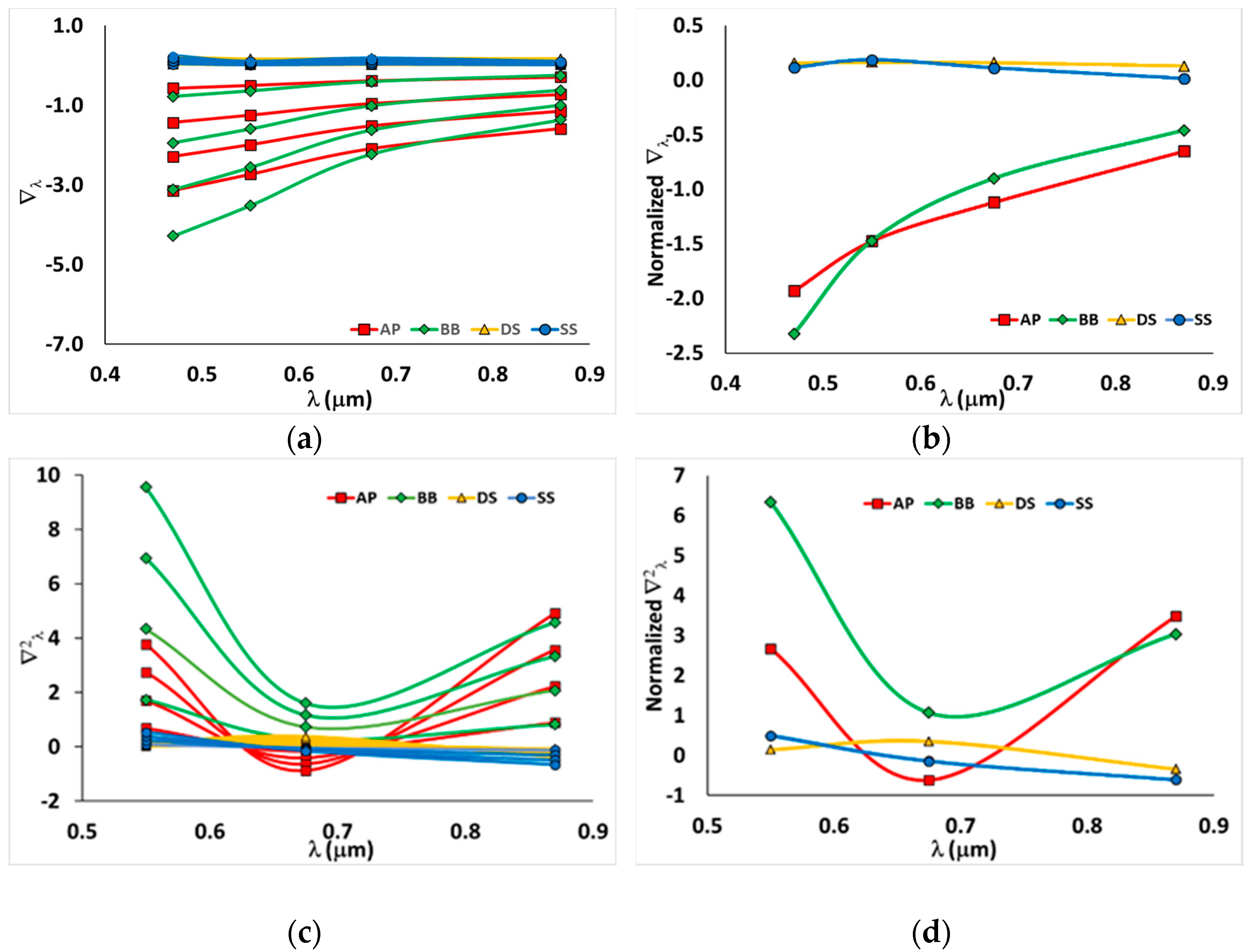
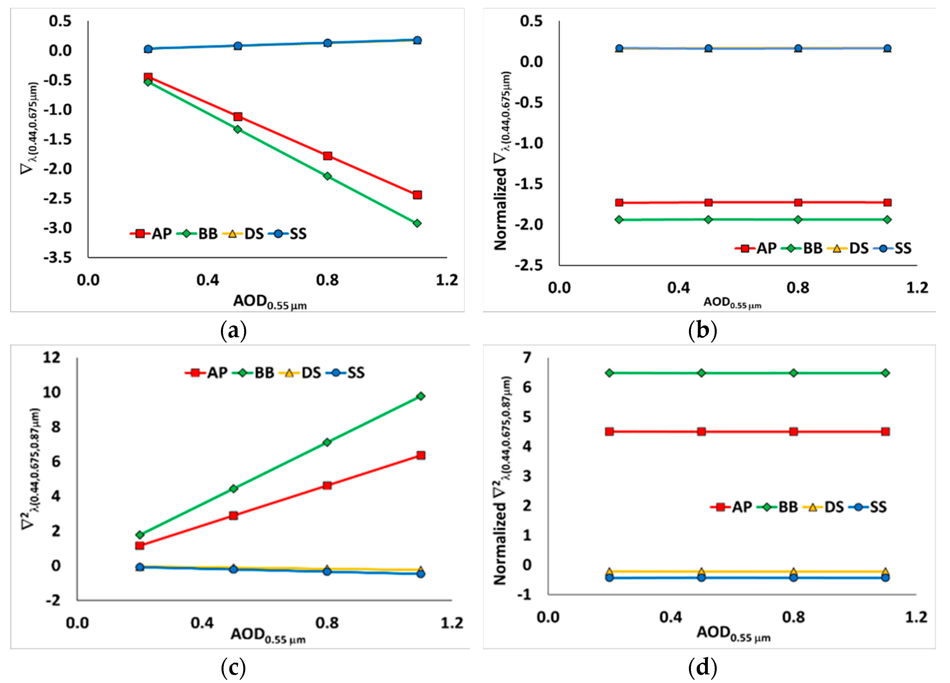
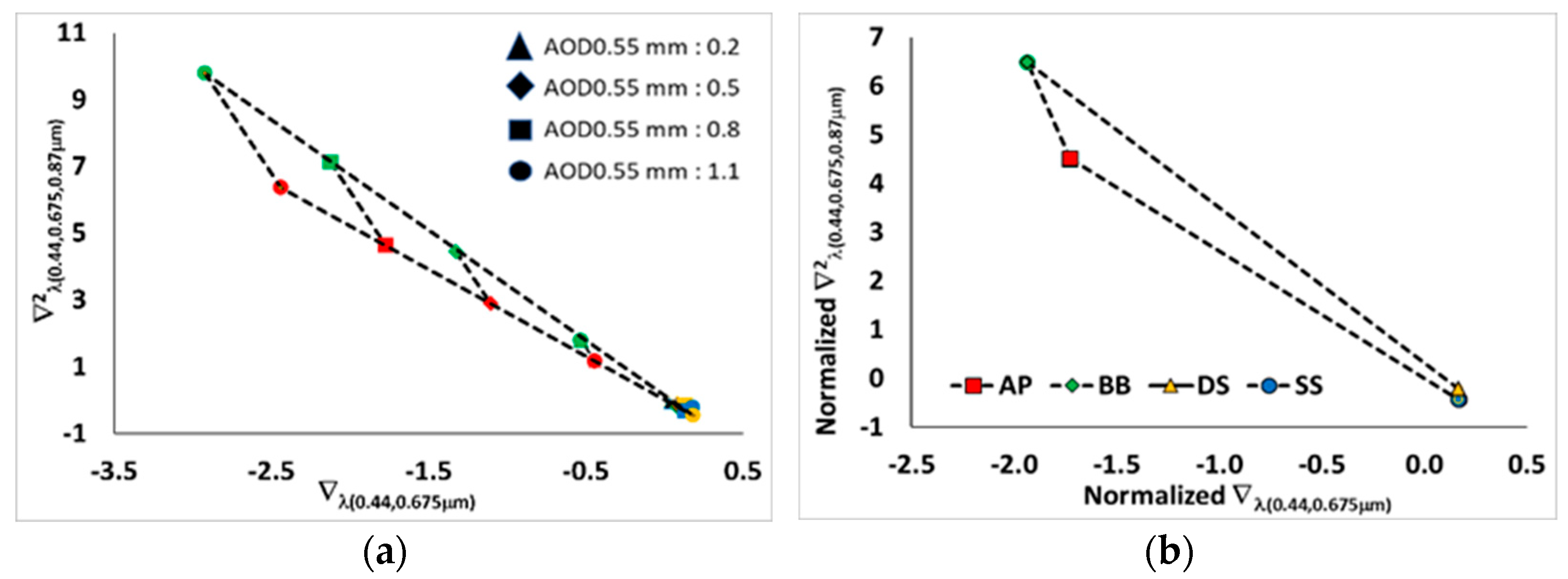
• Spectral derivatives explored the characteristics of each aerosol type through absorption between the wavelength pairs. Aerosol loadings governed the magnitude of spectral derivatives such as NDAI (Figure 4a). Based on Equation (2), NDAI was a function of particle size (Angstrom exponent) and also the first-order derivative of AODs at a logarithmic scale. The second-order derivatives compensated for the absence of SSA, and successfully partitioned aerosols based on their radiative characteristics. After normalization, the spectral derivatives converged and had their own individual values that served to differentiate them (Figure 4b).
• The simulation of a radiative transfer model such as the 6S model was advantageous to experiment or predict the radiative transfer of light-scattering absorption through the Earth’s atmosphere, according to the response variables used for fitting. However, in this study, there was a slight discrepancy in magnitudes between the spectral derivatives calculated from the 6S model and the satellite measurements (AERONET and satellite observation). This minor disagreement was due to the 6S model being operated under ideal atmospheric conditions. Nevertheless, a comparison of the results from simulation and the observation showed they were similar.
• SS had similarities to DS including its optical particle size and its imaginary part of the refractive index, but after normalization, both had their own individual optical characteristics. The particle size computed from longer wavelength pairs (e.g., AE_{(0.675–1.02μm),} AE_{(0.87,2.13μm)}) could illustrate more obvious differences in magnitudes between DS and SS. BB and AP were less complicated to discriminate, as although they have similar particle sizes, they have different radiative effects.
• Each aerosol species indicated different characteristics in radiative forcing and efficiency at the TOA, the BOA, and the atmosphere itself. Radiative forcing is dependent not only on the amount of radiation entering the atmosphere but also on the mass concentration of aerosol perturbing the atmosphere. To remove the influence of aerosol loading in the calculations of radiative forcing, AOD_0.55μm was used to normalize the radiative forcing, which is called radiative forcing efficiency. At the TOA, SS had the smallest magnitude, −36 W/m², while AP had the lowest magnitude at the BOA but the highest in the atmosphere, with −66.2 and 32.5 W/m², respectively. In addition, the relationship between AOD_0.55μm and radiative forcing efficiency was illustrated to compare the forcing abilities of the different aerosol types. The relationships were marked by negative slopes indicating negative relationships. When the AOD_0.55μm was increasing, the SWARFE was decreasing, and vice versa. Figure 7b,c shows the relationship between RF and AOD_0.55μm for the different aerosol types. The slopes of the best-fit line, shown by dashed lines, give the average forcing efficiency, as estimated by Equation (7). SS generated the most efficient radiative cooling effects, as it had the steepest slope, on the TOA among the three aerosol types. For instance, when the AOD_0.55μm is 0.2, the aerosol RFs from SS, BB, DS, and AP are estimated to be −7.35, −6.73, −6.19, and −6.04 W/m², respectively. This means that with the same magnitude of AOD_0.55μm, SS produced the strongest cooling effect at TOA compared to the other aerosol species. At BOA, AP had the greatest cooling effect among the other three aerosol constituents. The emissions and corresponding radiative effects of SS will change dynamically depending on the availability of driving factors such as global warming and climate change.
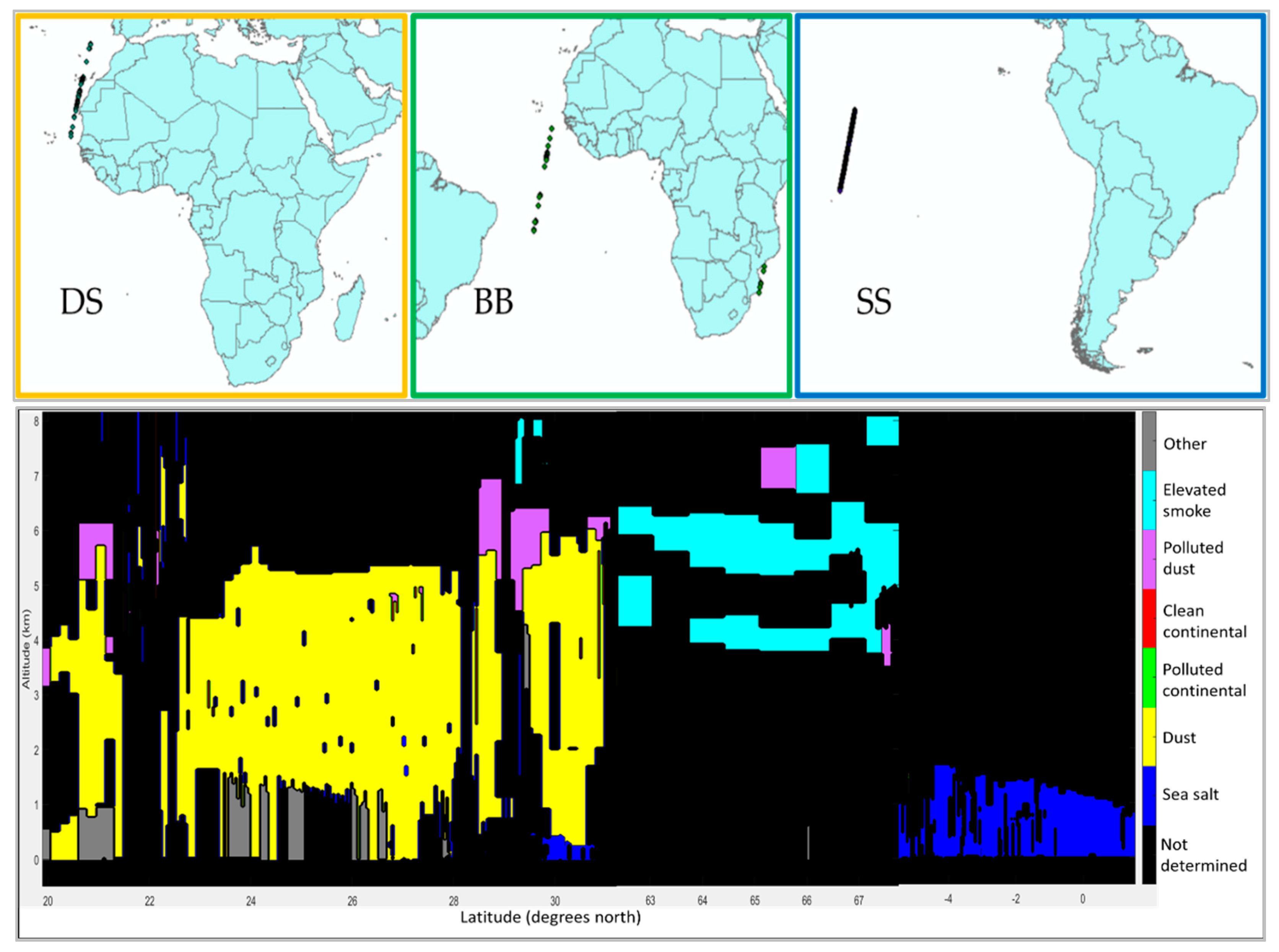
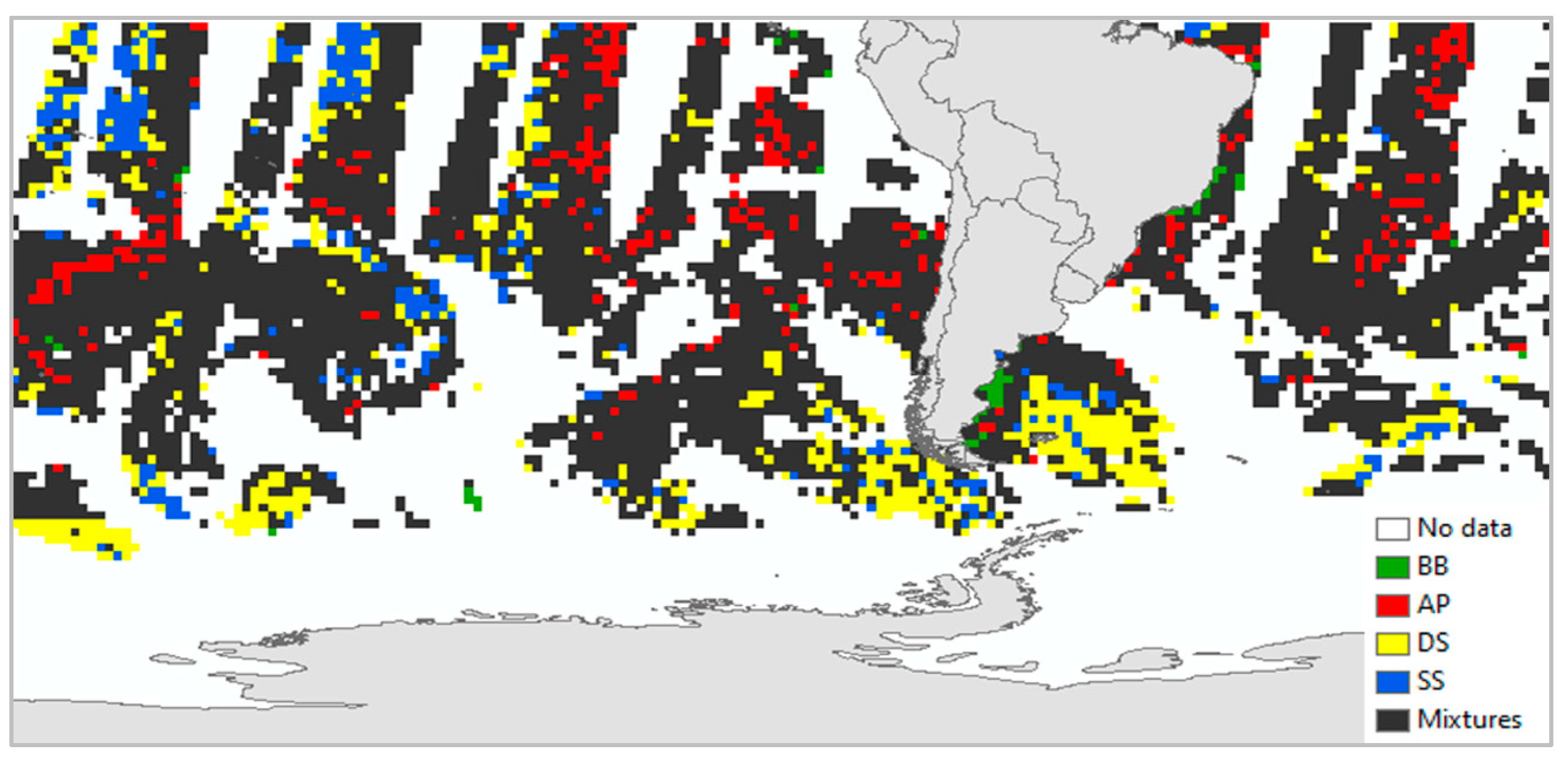
• MODIS aerosol products (e.g., MOD04_L2, MOD08_D3) providing daily observations of AOD globally can overcome the absence or limited coverage from surface monitoring, particularly over the ocean. It can be used to monitor the spatial and temporal distribution of SS and other aerosol types. The first- and second-order derivatives calculated from spectral AODs can be useful and practical tools to compensate the absence of SSA due to the dark target algorithm applied for AOD retrieval over the ocean. In addition, the spectral derivatives optimistically discriminate major components of aerosol species (e.g., BB, AP, DS, SS) and map out their distributions and corresponding radiative forcings. Continuing global aerosol monitoring over the ocean is required to better understand the spatio-temporal distribution of aerosol types and their radiative effects in a changing climate.

References

1. Liu, S.; Liu, C.-C.; Froyd, K.D.; Schill, G.P.; Murphy, D.M.; Bui, T.P.; Dean-Day, J.M.; Weinzierl, B.; Dollner, M.; Diskin, G.S.; et al. Sea spray aerosol concentration modulated by sea surface temperature. Proc. Natl. Acad. Sci. USA 2021, 118, e2020583118. [Google Scholar] [CrossRef]
2. Schiffer, J.M.; Mael, L.E.; Prather, K.A.; Amaro, R.E.; Grassian, V.H. Sea spray aerosol: Where marine biology meets atmospheric chemistry. ACS Cent. Sci. 2018, 4, 1617–1623. [Google Scholar] [CrossRef]
3. Andreae, M.O.; Jones, C.D.; Cox, P.M. Strong present-day aerosol cooling implies a hot future. Nature 2005, 435, 1187–1190. [Google Scholar] [CrossRef] [PubMed]
4. Boucher, O.D.; Randall, P.; Artaxo, C.; Bretherton, G.; Feingold, P.; Forster, V.-M.; Zhang, X.Y. Clouds and Aerosols. In Climate Change 2013: The Physical Science Basis. Contribution of Working Group I to the Fifth Assessment Report of the Intergovernmental Panel on Climate Change; Cambridge University Press: Cambridge, UK; New York, NY, USA, 2013. [Google Scholar]
5. Frey, M.M.; Norris, S.J.; Brooks, I.M.; Anderson, P.S.; Nishimura, K.; Yang, X.; Wolff, E.W. First direct observation of sea salt aerosol production from blowing snow above sea ice. Atmos. Chem. Phys. 2020, 20, 2549–2578. [Google Scholar] [CrossRef] [Green Version]
6. Metzger, S.; Mihalopoulos, N.; Lelieveld, J. Importance of mineral cations and organics in gas-aerosol partitioning of reactive nitrogen compounds: Case study based on MINOS results. Atmos. Chem. Phys. 2006, 6, 2549–2567. [Google Scholar] [CrossRef] [Green Version]
7. Liao, H.; Seinfeld, J.H. Global impacts of gas-phase chemistry-aerosol interactions on direct radiative forcing by anthropogenic aerosols and ozone. J. Geophys. Res. 2005, 110, D18208. [Google Scholar] [CrossRef] [Green Version]
8. Xu, L.; Penner, J.E. Global simulations of nitrate and ammonium aerosols and their radiative effects. Atmos. Chem. Phys. 2012, 12, 9479–9504. [Google Scholar] [CrossRef] [Green Version]
9. Lowe, D.; Archer-Nicholls, S.; Morgan, W.; Allan, J.; Utembe, S.; Ouyang, B.; Aruffo, E.; Le Breton, M.; Zaveri, R.A.; Di Carlo, P.; et al. WRF-Chem model predictions of the regional impacts of N2O5 heterogeneous processes on night-time chemistry over north-western Europe. Atmos. Chem. Phys. 2015, 15, 1385–1409. [Google Scholar] [CrossRef] [Green Version]
10. Chen, Y.; Cheng, Y.; Ma, N.; Wei, C.; Ran, L.; Wolke, R.; Größ, J.; Wang, Q.; Pozzer, A.; Denier van der Gon, H.A.; et al. Natural sea-salt emissions moderate the climate forcing of anthropogenic nitrate. Atmos. Chem. Phys. 2020, 20, 771–786. [Google Scholar] [CrossRef] [Green Version]
11. IPCC. Climate Change 2013: The Physical Science Basis. Contribution of Working Group I to the Fifth Assessment Report of the Intergovernmental Panel on Climate Change; Report; Stocker, T.F., Qin, D.H., Plattner, G.K., Tignor, M.M.B., Allen, S.K., Boschung, J., Nauels, A., Xia, Y., Bex, V., Midgley, P.M., Eds.; Cambridge University Press: New York, NY, USA, 2013; Available online: http://www.ipcc.ch/report/ar5 (accessed on 21 June 2022).
12. Struthers, H.; Ekman, A.M.L.; Glantz, P.; Iversen, T.; Kirkevåg, A.; Seland, Ø.; Mårtensson, E.M.; Noone, K.; Nilsson, E.D. Climate-induced changes in sea salt aerosol number emissions: 1870 to 2100. J. Geophys. Res. Atmos. 2013, 118, 670–682. [Google Scholar] [CrossRef]
13. Smirnov, A.; Holben, B.N.; Kaufman, Y.J.; Dubovik, O.; Eck, T.F.; Slutsker, I.; Pietras, C.; Halthore, R.N. Optical properties of atmospheric aerosol in maritime environments. J. Atmos. Sci. 2002, 59, 501–523. Available online: https://journals.ametsoc.org/view/journals/atsc/59/3/1520-0469_2002_059_0501_opoaai_2.0.co_2.xml (accessed on 21 May 2022). [CrossRef] [Green Version]
14. Quinn, P.K.; Coffman, D.J.; Kapustin, V.N.; Bates, T.S.; Covert, D.S. Aerosol optical properties in the marine boundary layer during the First Aerosol Characterization Experiment (ACE 1) and the underlying chemical and physical aerosol properties. J. Geophys. Res. 1998, 103, 16547–16563. [Google Scholar] [CrossRef]
15. Platnick, S.; King, M.; Meyer, K.G.; Wind, G.; Amarasinghe, N.; Marchant, B.; Arnold, G.T.; Zhang, Z.; Hubanks, P.A.; Ridgway, B.; et al. MODIS Atmosphere L3 Daily Product. In NASA MODIS Adaptive Processing System; Goddard Space Flight Center: Greenbelt, MD, USA, 2015. [Google Scholar] [CrossRef]
16. Sayer, A.M.; Hsu, N.C.; Lee, J.; Kim, W.V.; Dutcher, S.T. Validation, stability, and consistency of MODIS collection 6.1 and VIIRS version 1 Deep Blue aerosol data over land. J. Geophys. Res. Atmos. 2019, 124, 4658–4688. [Google Scholar] [CrossRef]
17. Zhou, Y.; Levy, R.C.; Remer, L.A.; Mattoo, S.; Shi, Y.; Wang, C. Dust aerosol retrieval over the oceans with the MODIS/VIIRS Dark-Target algorithm: 1. Dust detection. Earth Space Sci. 2020, 7, e2020EA001221. [Google Scholar] [CrossRef]
18. Kim, M.-H.; Omar, A.H.; Tackett, J.L.; Vaughan, M.A.; Winker, D.M.; Trepte, C.R.; Hu, Y.; Liu, Z.; Poole, L.R.; Pitts, M.C.; et al. The CALIPSO version 4 automated aerosol classification and lidar ratio selection algorithm. Atmos. Meas. Tech. 2018, 11, 6107–6135. [Google Scholar] [CrossRef] [PubMed] [Green Version]
19. Winker, D.M.; Pelon, J.; Coakley, J.A., Jr.; Ackerman, S.A.; Charlson, R.J.; Colarco, P.R.; Flamant, P.; Fu, Q.; Hoff, R.M.; Kittaka, C.; et al. The CALIPSO mission: A global 3D view of aerosols and clouds. Bull. Amer. Meteor. Soc. 2010, 91, 1211–1229. [Google Scholar] [CrossRef]
20. Balarabe, M.; Abdullah, K.; Nawawi, M. Seasonal variations of aerosol optical properties and identification of different aerosol types based on AERONET data over Sub-Sahara West-Africa. Atmos. Clim. Sci. 2015, 6, 13–28. [Google Scholar] [CrossRef] [Green Version]
21. Boselli, A.; Caggiano, R.; Cornacchia, C.; Madonna, F.; Mona, L.; Macchiato, M.; Pappalardo, G.; Trippetta, S. Multi year sun-photometer measurements for aerosol characterization in a Central Mediterranean site. Atmos. Res. 2012, 104, 98–110. [Google Scholar] [CrossRef]
22. Eck, T.; Holben, B.; Reid, J.; Dubovik, O.; Smirnov, A.; O’neill, N.; Slutsker, I.; Kinne, S. Wavelength dependence of the optical depth of biomass burning, urban, and desert dust aerosols. J. Geophys. Res. Atmos. 1999, 104, 31333–31349. [Google Scholar] [CrossRef]
23. Kalapureddy, M.C.R.; Kaskaoutis, D.G.; Raj, P.E.; Devara, P.C.S.; Kambezidis, H.D.; Kosmopoulos, P.G.; Nastos, P.T. Identification of aerosol type over the Arabian Sea in the premonsoon season during the Integrated Campaign for Aerosols, Gases and Radiation Budget (ICARB). J. Geophys. Res. Atmos. 2009, 114, D17203. [Google Scholar] [CrossRef] [Green Version]
24. Lin, T.-H.; Tsay, S.-C.; Lien, W.-H.; Lin, N.-H.; Hsiao, T.-C. Spectral derivatives of optical depth for partitioning aerosol type and loading. Remote Sens. 2021, 13, 1544. [Google Scholar] [CrossRef]
25. Kokhanovsky, A. Aerosol Optics: Light Absorption and Scattering by Particles in the Atmosphere; Springer Praxis: Chichester, UK, 2008; p. 2163. [Google Scholar]
26. Montilla, E.; Mogo, S.; Cachorro, V.; Lopez, J.; de Frutos, A. Absorption, scattering and single scattering albedo of aerosols obtained from in situ measurements in the subarctic coastal region of Norway. Atmos. Chem. Phys. Discuss. 2011, 11, 2161–2182. [Google Scholar] [CrossRef] [Green Version]
27. Huang, X.; Song, Y.; Zhao, C.; Li, M.; Zhu, T.; Zhang, Q.; Zhang, X. Pathways of sulfate enhancement by natural and anthropogenic mineral aerosols in China. J. Geophys. Res. Atmos. 2014, 119, 14165–14179. [Google Scholar] [CrossRef]
28. Li, L.; Li, Z.; Chang, W.; Ou, Y.; Goloub, P.; Li, C.; Li, K.; Hu, Q.; Wang, J.; Wendisch, M. Aerosol solar radiative forcing near the Taklimakan Desert based on radiative transfer and regional meteorological simulations during the Dust Aerosol Observation-Kashi campaign. Atmos. Chem. Phys. 2020, 20, 10845–10864. [Google Scholar] [CrossRef]
29. Kotchenova, S.; Vermote, E. Validation of a vector version of the 6S radiative transfer code for atmospheric correction of satellite data. Part II: Homogeneous Lambertian and anisotropic surfaces. Appl. Opt. 2007, 46, 4455–4464. [Google Scholar] [CrossRef] [PubMed] [Green Version]
30. Kotchenova, S.; Vermote, E.; Matarrese, R.; Klemm, F., Jr. Validation of a vector version of the 6S radiative transfer code for atmospheric 470 correction of satellite data. Part I: Path radiance. Appl. Opt. 2006, 45, 6762–6774. [Google Scholar] [CrossRef] [PubMed] [Green Version]
31. Smirnov, A.; Holben, B.N.; Giles, D.M.; Slutsker, I.; O’Neill, N.T.; Eck, T.F.; Macke, A.; Croot, P.; Courcoux, Y.; Sakerin, S.M.; et al. Maritime aerosol network as a component of AERONET—First results and comparison with global aerosol models and satellite retrievals. Atmos. Meas. Tech. 2011, 4, 583–597. [Google Scholar] [CrossRef] [Green Version]
32. Hansell, R.A.S.-C.; Tsay, P.; Pantina, J.R.; Lewis, Q.J.; Herman, J.R. Spectralderivative analysis of solar spectroradio-metric measurements: Theoretical basis. J. Geophys. Res. Atmos. 2014, 119, 8908–8924. [Google Scholar] [CrossRef]
33. Ångström, A. The parameters of atmospheric turbidity. Tellus 1964, 16, 64–75. [Google Scholar] [CrossRef] [Green Version]
34. Altaratz, O.; Bar-Or, R.Z.; Wollner, U.; Koren, I. Relative humidity and its effect on aerosol optical depth in the vicinity of convective clouds. Environ. Res. Lett. 2013, 8, 034025. [Google Scholar] [CrossRef]
35. Gassó, K.S.; Hegg, D.A.; Covert, D.S.; Collins, D.; Noone, K.J.; Öström, E.; Schmid, B.; Russell, P.B.; Livingston, J.M.; Durkee, P.A.; et al. Influence of humidity on the aerosol scattering coefficient and its effect on the upwelling radiance during ACE-2. Tellus B Chem. Phys. Meteorol. 2000, 52, 546–567. [Google Scholar] [CrossRef]
36. Xue, Z.; Kuze, H.; Irie, H. Retrieval of aerosol optical thickness with custom aerosol model using SKYNET Data over the Chiba area. Atmosphere 2021, 12, 1144. [Google Scholar] [CrossRef]
37. Zhang, L.; Li, J.; Jiang, Z.; Dong, Y.; Ying, T.; Zhang, Z. Clear-sky direct aerosol radiative forcing uncertainty associated with aerosol vertical distribution based on CMIP6 models. J. Clim. 2022, 35, 3021–3035. [Google Scholar] [CrossRef]
38. Pilinis, C.K.; Seinfeld, J.H.; Grosjean, D. Water content of atmospheric aerosols. Atmos Environ. 1989, 23, 1601–1606. [Google Scholar] [CrossRef]
39. Cheng, Y.F.; Wiedensohler, A.; Eichler, H.; Heintzenberg, J.; Tesche, M.; Ansmann, A.; Wendisch, M.; Su, H.; Althausen, D.; Herrmann, H.; et al. Relative humidity dependence of aerosol optical properties and direct radiative forcing in the surface boundary layer at Xinken in Pearl River Delta of China: An observation based numerical study. Atmos. Environ. 2008, 42, 6373–6397. [Google Scholar] [CrossRef]
40. Topping, D.O.; McFiggans, G.B.; Coe, H. A curved multi-component aerosol hygroscopicity model framework: Part 1—Inorganic compounds. Atmos. Chem. Phys. 2005, 5, 1205–1222. [Google Scholar] [CrossRef] [Green Version]
41. Topping, D.O.; McFiggans, G.B.; Coe, H. A curved multicomponent aerosol hygroscopicity model framework: Part 2—Including organic compounds. Atmos. Chem. Phys. 2005, 5, 1223–1242. [Google Scholar] [CrossRef] [Green Version]
42. Ramachandran, S.; Srivastava, R. Influences of external vs. core-shell mixing on aerosol optical properties at various relative humidities. Environ. Sci. Process. Impacts 2013, 15, 1070–1077. [Google Scholar] [CrossRef]
43. Ghahremaninezhad, R.; Gong, W.; Galí, M.; Norman, A.-L.; Beagley, S.R.; Akingunola, A.; Zheng, Q.; Lupu, A.; Lizotte, M.; Levasseur, M.; et al. Dimethyl sulfide and its role in aerosol formation and growth in the Arctic summer—A modelling study. Atmos. Chem. Phys. 2019, 19, 14455–14476. [Google Scholar] [CrossRef] [Green Version]
44. Bullard, J.E.; Baddock, M.; Bradwell, T.; Crusius, J.; Darlington, E.; Gaiero, D.; Gassó, S.; Gisladottir, G.; Hodgkins, R.; McCulloch, R.; et al. High-latitude dust in the Earth system. Rev. Geophys. 2016, 54, 447–485. [Google Scholar] [CrossRef] [Green Version]
45. McGregor, D. Book review: World atlas of desertification, 2nd edn., edited by N. J. Middleton and D. S. G. Thomas. Arnold, London for United Nations Environment Programme, 1997. ISBN 0-34069166-2, £145·00 (hardback), x+182 pp. Land Degrad. Dev. 1999, 10, 177–178. [Google Scholar] [CrossRef]
46. Mirzabaev, A.; Wu, J.; Evans, J.; Garcia-Oliva, F.; Hussein, I.A.; Iqbal, M.H.; Kimutai, J.; Knowles, T.; Meza, F.; Nedjraoui, D.; et al. Desertification. In Climate Change and Land: An IPCC Special Report on Climate Change, Desertification, Land Degradation, Sustainable Land Management, Food Security, and Greenhouse Gas Fluxes in Terrestrial Ecosystems; Shukla, P.R., Skea, J., Buendia, E.C., Masson-Delmotte, V., Pörtner, H.-O., Roberts, D.C., Zhai, P., Slade, R., Connors, S., van Diemen, R., et al., Eds.; IPCC: Geneva, Switzerland, 2019; in press. [Google Scholar]
47. Rhein, M.S.R.; Rintoul, S.; Aoki, E.; Campos, D.; Chambers, R.A.; Feely, S.; Gulev, G.C.; Johnson, S.A.; Josey, A.; Kostianoy, C.; et al. Observations: Ocean. In Climate Change 2013: The Physical Science Basis. Contribution of Working Group I to the Fifth Assessment Report of the Intergovernmental Panel on Climate Change; Stocker, T.F., Qin, D., Plattner, G.-K., Tignor, M., Allen, S.K., Boschung, J., Nauels, A., Xia, Y., Bex, V., Midgley, P.M., Eds.; Cambridge University Press: Cambridge, UK; New York, NY, USA, 2013. [Google Scholar]
Figure 1. The simulated spectral aerosol optical depths (AODs) at 0.44, 0.47, 0.55, 0.66, 0.675, 0.87, and 1.02 μm for anthropogenic pollutant (AP, red), biomass burning (BB, green), dust (DS, yellow), and sea salt (SS, blue) under initial AOD0.55μm values of 0.2, 0.5, 0.8, and 1.1 from the second simulation of a satellite signal in solar spectrum (6S) radiative transfer model with the experimental dataset.
Remotesensing 14 03188 g001
Figure 2. The first and second-order derivatives before (a,c) and after normalization (b,d) of 4 different aerosol constituents: anthropogenic pollutant (AP), biomass burning (BB), dust (DS), and sea salt (SS).
Remotesensing 14 03188 g002
Figure 3. The comparison of first-order derivatives with respect to aerosol loadings (AOD0.55μm) before (a) and after normalization with AOD0.44μm (b) and the comparison of the second-order derivative wavelengths before (c) and after normalization with AOD0.44μm (d).
Remotesensing 14 03188 g003
Figure 4. Relationships between the first and second-order derivatives before (a) and after (b) normalization with AOD0.44μm for each aerosol type: anthropogenic pollutant (AP: red), biomass burning (BB: green), dust (DS: yellow), and sea salt (SS: blue) under various AOD0.55μm inputs (triangle: 0.2, rhombus: 0.5, square: 0.8, and round: 1.1).
Remotesensing 14 03188 g004
Figure 5. Tracks of CALIPSO subtypes for dust (DS), biomass burning (BB), and sea salt (SS) (upper), and vertical aerosol subtypes for the corresponding tracks (lower).
Remotesensing 14 03188 g005
Figure 6. Distribution of aerosol types: anthropogenic pollutant (AP), biomass burning (BB), dust (DS), sea salt (SS), and mixtures based on their spectral derivatives calculated from MODIS daily aerosol products (MOD08_D3).
Remotesensing 14 03188 g006
Figure 7. The shortwave aerosol radiative forcing efficiency of each aerosol species (a), and the relationship between the shortwave aerosol radiative forcing efficiency (SWARFE) and AOD0.55μm at the top of the atmosphere (TOA) (b) and the bottom of the atmosphere (BOA) (c).
Remotesensing 14 03188 g007