Article

Kinematic Galileo and GPS Performances in Aerial, Terrestrial, and Maritime Environments

1
Department of Geosciences, Environment and Spatial Planning, Faculty of Sciences, University of Porto, 4169-007 Porto, Portugal
2
Interdisciplinary Centre of Marine and Environmental Research (CIIMAR/CIMAR), Faculty of Sciences, University of Porto, 4450-208 Matosinhos, Portugal
3
European Union Agency for the Space Programme, Galileo Reference Centre, Zwarteweg 53, 2201 AA Noordwijk, The Netherlands
4
GeoSNav Laboratory, Department of Engineering and Architecture, University of Trieste, Via Valerio 6/2, 34127 Trieste, Italy
5
Institute of Space Science, 409 Atomistilor Street, 077125 Magurele, Romania
6
Faculty of Aerospace Engineering, University Politehnica of Bucharest, 313 Splaiul Independentei, 060042 Bucharest, Romania
7
Astronomical Observatory, Faculty of Sciences, University of Porto, 4430-146 Vila Nova de Gaia, Portugal
8
Romanian Space Agency, 21–25 Mendeleev Str., 010362 Bucharest, Romania
*
Author to whom correspondence should be addressed.
Remote Sens. 2022, 14(14), 3414; https://doi.org/10.3390/rs14143414
Submission received: 10 June 2022 / Revised: 11 July 2022 / Accepted: 12 July 2022 / Published: 16 July 2022
(This article belongs to the Special Issue Satellite Navigation and Signal Processing)

Abstract

:
On 15 December 2016, the European Commission (EC) declared the provision of the Galileo Initial Services (IS). This marked a historical milestone in the Galileo program, towards the reaching of its Full Operational Capability. This allows users to navigate with performance-accuracy levels either matching or exceeding those obtained with other GNSS. Under the delegation of the EC, the European Union Agency for the Space Programme (EUSPA) has assumed the role of the Galileo Service Provider. As part of this service provision, the primary mission of the Galileo Reference Centre (GRC) is to provide the EUSPA and the EC with independent means for monitoring and evaluating the performance of the Galileo services, the quality of the signals in space, and the performance of other GNSS. This mission includes significant contributions from cooperating entities in the European Union (EU) Member States (MS), Norway and Switzerland. In particular, for a detailed assessment of the Galileo performance, these contributions include (but are not limited to) periodic dynamic campaigns in three different environments (aerial, terrestrial, and maritime). These campaigns were executed in the frame of the GRC-MS Project and use multi-constellation receivers to compare the navigation performance obtained with different GNSS. The objective of this paper is to present the numerical results obtained from these campaigns, together with several considerations about the experimental setup, the methodology for the estimation of the reference («actual») trajectory, and the reasons for possible performance degradations.

1. Introduction

Satellite navigation is playing a significant role in the high-precision navigation, positioning, and timing being used in various fields of activities, considering both static and dynamic applications [1]. Civilian global use and dependence on GNSS began in the 2000s, when more events occurred. These included: the decision of U.S.A. to discontinue the Selective Availability of GPS system [2], the starting point of the use of the Russian GLONASS system for civilian users and mass-market applications [3], and the completion of the construction of China’s first step on the path to developing a navigation satellite system, BeiDou, followed by other development phases, with BDS-3 construction, which was fully completed in 2020 [4].
Understanding the large market potential, the European Union (EU) decided in the early 2000s to develop its own satellite navigation infrastructure, Galileo. With this GNSS system, the EU aims at owning and providing an independent positioning/navigation service under civilian control, which is completely interoperable with the GPS, the GLONASS, and the BeiDou positioning systems [5]. Different services are designed to be provided by the Galileo system once it is fully operational. Of these, the Initial Open Service (OS) declaration on 15 December 2016 marked a historical milestone in the Galileo program. The Galileo OS is freely available for mass-market applications of synchronization and positioning. It does not require any authorization and can be used by anyone equipped with an adequate receiver [6]. Kinematic applications represent one of the main domains that can benefit from the advantages of the Galileo OS. In this context, it is of high interest to study the Galileo-only performances, as well as the multi-GNSS performances, for the kinematic applications using different positioning methods.
As the Galileo OS is a relatively recent milestone of the Galileo system, since the launch of the first Galileo satellites, the outcomes of the Galileo mission at different stages of development were analyzed, also considering the performance of combined multi-GNSS solutions for kinematic applications. Therefore, in 2012, Odijk et al. [7] presented the results of mixed GPS + GIOVE single-frequency RTK, using data from the Galileo System Test Bed (GSTB-V2) implementation phase. After the launch of the first four Galileo operational satellites, Rabbou and El-Rabbany [8] analyzed the improvements that these satellites, available in 2015, brought to a GPS PPP model, for static and kinematic applications in urban environments. The same authors, in [9], developed undifferenced and Between-Satellite Single-Difference (BSSD) ionosphere-free PPP models using multi-GNSS observations. Compared to the undifferenced PPP model, the accuracy of the GPS/Galileo BSSD PPP model was observed to be improved. Multi-GNSS PPP performance evaluation was analyzed in other studies, such as [10,11]. A multi GNSS single-frequency RTK study was presented in [12]. The performance of Galileo PPP using different frequencies was also examined in more recent studies, including triple-frequency, triple-constellation Precise-Point Positioning–Ambiguity Resolution (PPP-AR) models [13], triple-frequency single-constellation PPP solutions [14], triple-frequency GPS/Galileo PPP models [15], dual- and multi-frequency and multi-constellations combinations [16], and changes from the PPP approach to PPP-AR [17], for precise static and kinematic applications.
The articles mentioned above are focused on a general analysis of the kinematic applications. As this paper investigates kinematic Galileo and GPS performances for specific environments, the state of the art on assessing Galileo performances for aerial, terrestrial, and maritime kinematic positioning applications was checked in the literature.
When searching for publications with analyses of airborne kinematic positioning using Galileo-only measurements, no results were found in the literature. Available works are related to GPS-only [18] or GNSS positioning based on the use of combinations of GPS with other GNSS system (e.g., GLONASS, Galileo and BDS) solutions [19,20], as well as INS/GNSS integration [21].
For the terrestrial domain, the results of a single-frequency kinematic performance comparison among the Galileo, GPS, and GLONASS systems using an MMS (Mobile Mapping System) generated a trajectory as reference, presented in [6]. It is stated that the Galileo system is characterized by a better planimetric performance with respect to the other systems, referred to by the reference trajectory [6]. The results of a vehicular test conducted in urban and suburban areas, with real-time computed kinematic GPS/Galileo PPP solutions, are presented in [22]. It was revealed that the GPS/Galileo solution had improvements of more than 45% in the east, north, and up directions, compared to the GPS-only solution.
As for the aerial and terrestrial domains, maritime kinematic positioning studies including Galileo measurements are not very numerous. Among the first studies, in 2008, in the frame of SEA Gate project, Galileo applications started to be developed and tested, broadcasting a Galileo-like signal [23,24,25]. Marila et al. [26] highlight some GNSS (GPS, GLONASS, Galileo, BeiDou) positioning aspects for the Intelligent Shipping Test Laboratory (ISTLAB), proposing the use of RTK with Virtual Reference Station (VRS) [26].
The aerial, terrestrial, and maritime kinematic positioning applications and results presented in this paper take into consideration the Galileo OS performances, as data-collection campaigns took place after 2019. This work is part of the GRC-MS (Galileo Reference Centre–Member States), a component of the Galileo Reference Centre (GRC) [27], which is presented in the following section.

1.1. Galileo Reference Centre

Under the delegation of the EC, the European Union Agency for the Space Programme (EUSPA) has assumed the role of the Galileo Service Provider. As the operator and the maintainer of the Galileo system, the primary mission of the EUSPA, through the Galileo Reference Centre (GRC), is performing independent monitoring and assessment of Galileo’s service provision [28]. It is fully independent of the system and of the operator, with respect to both the technical solution and operations. The GRC also provides service performance expertise to the Galileo Programme, support to investigations of service performance and service degradations and archival of relevant service performance data over the operational lifetime of the system. Where feasible, the GRC also assesses the compatibility and interoperability between Galileo and other GNSS [27].
The GRC comprises a core facility, which is located in Noordwijk, Netherlands, and integrates data and products from cooperating entities from the EU Member States, Norway and Switzerland (MS). The countries that have established a framework partnership agreement to support the GRC are indicated in Figure 1.
Contributions from MS support everyday operations and specific campaigns. These contributions from the GRC-MS Project include the following:
  • data provision from a regional and worldwide network
  • orbits and clock reference products
  • consolidated navigation («Broadcast Galileo» BRDG) files
  • KPIs Generation
  • Signal in Space (SIS) monitoring
  • Satellite Laser Ranging (SLR) campaign
  • ionospheric monitoring:
    ionospheric reference products, and
    NeQuick G model performance
  • data provision from measurement campaign (based using vehicles, vessels and aircraft)
  • expertise available at the Member-State level.
An important part of Galileo’s performance assessment is the evaluation of the performance experienced by a generic user in different propagation environments. For that reason, in support of GRC, in the frame of the GRC-MS project, periodic kinematic campaigns using multi-constellation satellite receivers are realized. The dynamic data-collection campaigns are conducted by three participating member states (Portugal, Italy, and Romania), in three different environments (aerial, terrestrial, and maritime, respectively). This article presents a comparison of the results obtained for each environment, considering the performance of Galileo used in conjunction with other GNSS systems, such as GPS, by different experimental dynamic activities. Starting from the user’s needs and requirements, which are presented in the next section, several considerations about the experimental setup and the methodology for the estimation of the reference («actual») trajectory are provided. These are complemented by numerical results and an analysis of the reasons for possible performance degradations.
Some ad hoc optimized hardware/software configurations were set up in order to achieve the best acquisition performances and test different satellite/signal combinations and processing options. The processed rover trajectories and the produced outputs were compared to two different reference trajectories. The first reference trajectory was obtained from GNSS/INS integrated high-performance solution, and it was used for the aerial and terrestrial data-collection campaigns. The second reference trajectory was a PPP solution, and it was used for all the data-collection campaigns (aerial, terrestrial, and maritime). More details about the reference trajectories can be found in Section 2.2 of this paper. The performed analysis revealed similar performances of the Galileo-only and GPS-only solutions, respectively, with better results for the Galileo-only solution in the more recent road campaigns. A multi-system solution (GPS and Galileo) is also analyzed. In this case, the best performance is obtained for the urban and maritime environments.
The next section deals with the user’s needs and requirements in the aerial, maritime, and terrestrial domains. These will be considered as a baseline for the performance observed in the kinematic applications during the measurement campaigns.

1.2. User Needs and Requirements in the Aerial, Maritime, and Terrestrial Domains

Kinematic applications demand adequate position requirements, which are transposed in terms of accuracy, integrity, availability, and continuity. These indicators have specific values and interpretations for each specific domain of transportation. Based on the authorities’ recommendations and the requirements of each domain (aeronautics, road transportation, and maritime), the GSA Market Report Issue 6, 2019 [29] presents the key user requirements for each mentioned domain, as outlined in the Table 1, Table 2 and Table 3.
During the airborne campaigns, presented later in this paper, no specific a priori requirements were set. The “performance-based navigation” requirements were used to analyze the performance of the Single-Point Positioning (SPP) solutions.
The navigation phases during the maritime campaigns presented in this paper were: coastal navigation (accuracy requirements up to 10 m), port navigation, and port approach, (accuracy requirements between 1 and 10 m) according to IMO A.915(22) [30].
The performance results of the dynamic campaigns were compared with the key user requirements for each domain.

2. Materials and Methods

2.1. Data-Collection Campaigns

The data for the aerial, terrestrial, and maritime campaigns were acquired on quarterly periods during 2019 and 2020. In this paper, the results from two quarterly data-collection campaigns in 2019 and two in 2020 are presented. Due to the COVID-19 pandemic, 2020 was an atypical year, and some delays were registered for some data-collection campaigns. Considering the objective of monitoring the Galileo performances, the location and the acquisition time were chosen to expose different situations (i.e., different Galileo satellites configuration, different surrounding areas during each type of campaign, and different meteorological conditions). The approximate duration of the data-collection campaigns is between 1 and 2 h. We considered the two-hour interval relevant for the purpose of our project, also including logistical and economic reasons (especially for the aerial campaign). Table 4 presents the approximate duration for each campaign, the PVT computation techniques, and the reference trajectory computation methods. Due to the specificity of the different data-collection campaigns, we tried to have sufficient number of Galileo satellites in the different countries. No other constraints were placed on the campaign planning, as we wanted to have different observation conditions, as specified above.

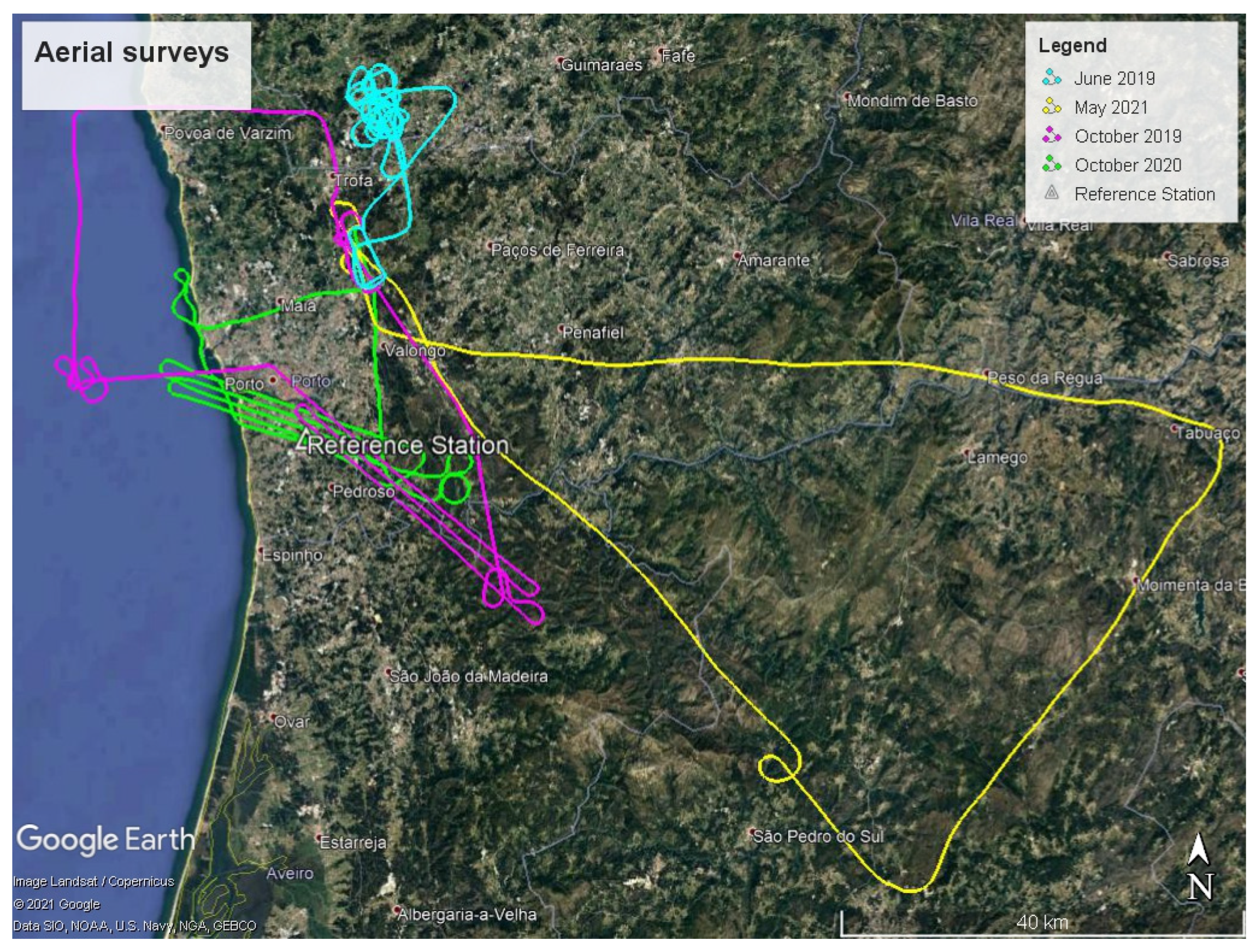
2.1.1. Experimental Setup for the Aerial Data-collection Campaigns

The airborne campaigns, conducted under the supervision of the Astronomical Observatory of the University of Porto (AOUP), took place in the Porto region, along the countryside and the coast (see Figure 2), using a CESSNA C210 airplane. The flight altitudes varied between 1000 ft (300 m) and 5000 ft (1500 m), with mean velocities of 200 km/h.
The GNSS receivers used in the different campaigns allowed the acquisition of all the frequencies from the Galileo, GPS, GLONASS, and BEIDOU constellations.
Figure 3 presents the hardware installed in the aircraft, which involves two GNSS/IMU units and two GNSS receivers (GPS dual frequency and GNSS multi frequency), as indicated in Table 5. The corresponding lever-arms are indicated in Figure 3.
The GNSS/IMU (Global Navigation Satellite System/Inertial Measurements Unit) systems allow the precise determination of the position and altitude of the aircraft or of the sensors onboard at each instant. The LN200 measurements, acquired at 200 Hz, and the POS system measurements, acquired at 64 Hz, were integrated with the GNSS-derived positions using algorithms based on EKF (Extended Kalman Filter) developed at FCUP (Porto, Portugal) in the LN200 case and the AEROcontrol software from IGI mbH (Kreuztal, Germany) in the POS case. These solutions were used as references.

2.1.2. Experimental Setup for the Terrestrial Data-Collection Campaigns

The researchers of the GeoSNav Lab, Department of Engineering and Architecture, University of Trieste, Italy, performed the terrestrial surveys using an MMS (Mobile Mapping System) along extra-urban and urban paths. The urban surveys took place in the Trieste city-center and the extra-urban surveys over the Karst plateau, at an average altitude of 375 m above mean sea level, with a good satellite visibility and signal-to-noise ratio (Figure 4).
The Mobile Mapping System uses the Applanix Corporation POS/LV (Position and Orientation System/Land Vehicles) System, a fully integrated, position and orientation system, with GNSS positioning integrated by inertial technology to generate stable, reliable, and repeatable positioning solutions for land-based vehicle applications (Figure 5). Designed to operate under the most difficult GNSS conditions in urban and suburban environments, it enables accurate positioning for road geometry, pavement inspection, GIS database and asset management, road surveying, and vehicle dynamics [31]. The integrated GNSS/IMU (Global Navigation Satellite System/Inertial Measurement Unit) is able to provide, epoch by epoch, the position and altitude of the vehicle. In addition to the two geodetic Trimble GNSS receivers and the Inertial System, there is also an odometer mounted on the rear-left wheel of the vehicle, measuring the traveled distance (Table 6). The inertial system integrates the GPS in the case of no satellite signal due to obstacles such as bridges, trees, or buildings, to provide positioning accuracies comparable to the ones obtainable through differential techniques [32,33]. A Kalman filter, which allows the user to gain the best solution at any time, performs the integration of each sensor’s data. GNSS data has a 1 Hz acquisition rate, while the odometer and the inertial system send data to the System CPU at a rate of 200 Hz.
All positioning data were referred to the Septentrio AsterX-U receiver PolaNt-x MF antenna phase center. This was completed to directly compare, epoch by epoch, the positions computed using the Septentrio AsterX-U receiver data (Septentrio, Leuven, Belgium) with the MMS reference trajectory.
The PCS (POS Computer System) (Applanix, Richmond Hill, ON, Canada) is the central element of the Applanix system: it acquires and processes data coming from the different sensors, providing the positioning and attitude parameters of the vehicles in real time and stores them for subsequent post-processing. The integrated inertial system is a Litton LN-200 fiber optic gyro IMU (Inertial Measurements Unit) (Northrop Grumman, Falls Church, VA, USA)with three accelerometers and three fiber-optic laser gyros (identical with the instrument used for the aerial data-collection campaigns). The odometer uses an optical sensor generating 1024 pulses per revolution. Its function is to estimate the run distance and, above all, to determine when the vehicle has come to a halt (ZUPD, Zero Velocity Update). Two geodetic GPS receivers send the data to the PCS for positioning and direction determination, the latter utilizing the GAMS (GPS Azimuth Measurement Subsystem) (Applanix, Richmond Hill, ON, Canada) software module.

2.1.3. Experimental Setup for the Maritime Data-Collection Campaigns

The maritime data-collection campaigns took place in the Romanian coastal waters of the Black Sea and in the port area, aside from the last-described campaign (Q4 2020), which took place in the open sea, at more than 50 nautical miles from the shore (Figure 6). All the campaigns were performed on board the “Cpt. Cdor Alexandru Catuneanu” vessel (Figure 7a), which is part of the fleet of the Romanian Maritime Hydrographic Directorate [34].
Considering the placement of the onboard sensors and the equipment of the vessel, the first step in the configuration of the GNSS data-collection campaign setup was to find the most suitable places for the GNSS antennas, considering the requirements mentioned in the IMO A.694(17) resolution [35]. As the most suitable placement, the GNSS antennas were installed on the bow lighting mast.
The GNSS equipment configuration includes two identical Septentrio AsteRx-U multi-constellation, multi-frequency receivers and two types of antennas. These are a high-precision geodetic antenna, i.e., PolaNt-x MF, and a choke ring antenna, i.e., Septentrio PolaNt Choke Ring B3/E6 antenna. Considering the available receivers and antennas, the first receiver was connected to the regular maritime antenna (as the main antenna), and the second receiver was connected to the choke ring antenna. To fulfil the protection standards and to assure the power supply need, the receivers were placed in a special rack in the control cabin. To prevent the effect of possible short power outages, a temporary external power supply was put together with the GNSS receivers in the rack (Figure 7b).
Table 7 contains the list of equipment used for the maritime data-collection campaigns.

2.2. Reference Solutions

To obtain a reference trajectory solution for the different data-collection campaigns, we used the CSRS-PPP (PPP—Precise-Point Positioning) service of the Canadian Geodetic Survey of Natural Resources Canada [36]. The CSRS-PPP processing algorithm uses precise orbits and clock and bias corrections derived from a global network of receivers and allows centimeter accuracies or even millimeter accuracies for long static sessions. The software tool finds itself the best available precise GNSS orbit ephemerides. The PPP version used in this work was launched on 16 August 2018 and was the first step of the modernization of this algorithm by using the ambiguity resolution (PPP-AR), featuring a faster convergence algorithm using external ionosphere information and processing multi-GNSS observations based on GPS and GLONASS observations. RINEX observation files from the GNSS receivers are provided to the PPP software as input. The obtained reference trajectory, which is a GPS/GLONASS double frequency (DF) solution, was compared with the different trajectory solutions obtained using single- and multi-frequency measurements from the Galileo-only, GPS-only, and Galileo+GPS systems. The solutions are all provided in the ITRF2014 system. The CSRS-PPP trajectory was used as reference trajectory for all the data-collection types.
For the aerial and terrestrial data-collection campaigns, an additional reference trajectory solution was computed using the GNSS/IMU measurements available on board the airplane (for the aerial campaign) and on board the MMS (for the terrestrial data-collection campaign). The GNSS/IMU system allowed the determination of a more reliable, accurate, and continuous trajectory of the moving platforms, also providing their attitude (roll, pitch, and yaw).
Both the reference trajectories have been used for performance evaluation.

2.3. GNSS Solutions

For all data-collection types, the differential GNSS solutions were obtained in post-processing mode, using two software tools.
For the aerial and maritime data, single- and triple-frequency differential GNSS solutions (SF and TF), using code- and carrier-phase measurements and the broadcast ephemeris, were obtained using the RTKLib software [37]. This software is an open-source software that allows the user to obtain multi-GNSS solutions in either the real-time or post-processing mode, supporting a lot of standard formats and protocols. The library tools can be used to process data or to obtain, convert, and analyze raw data and solutions. For data processing we used the Double-Difference approach. The software uses ionospheric and tropospheric models for computing the propagation errors and applies an EKF (Extended Kalman Filter) filter to obtain the final kinematic solutions. The following settings were applied to obtain the differential TF solutions with RTKLib for the Galileo (E1/E5a/E5b), GPS (L1/L2/L5), and GNSS (E1/L1, E5a/L5, E5b/L2, E6): 10° elevation mask; ionospheric corrections based on the Klobuchar model [38] (broadcast parameters); tropospheric corrections using the Saastamoinen model [39]; satellite and receiver antenna correction using the ANTEX ngs14.atx file. The RTKLib options for Earth tides corrections, using the IERS Conventions [40], and EOP (Earth Orientation Parameters), from IGS-ERP (International GNSS Service—Earth Rotation Parameters) were also used in this processing.
Considering the aerial data-collection campaigns in the Porto area, for the differential positioning approach, a permanent station located at the Astronomical Observatory grounds, less than 70 km from the test flight areas, was used as reference station.
The reference station used for the differential positioning approach during the maritime data collection was Constanta permanent GNSS station, part of the ROMPOS (Romanian Position Determination System) [41] and of EUREF Permanent GNSS Network [42]. Due to the fact that, during the maritime data-collection campaigns, different navigation phases were considered, in the case of open sea (Q4 2020), the test area was located more than 100 km from the reference station. For the other approaches (port and coastal navigation), the reference station was situated less than 35 km from the test area.
For the terrestrial data collection, the epoch-by-epoch DF differential GNSS solutions were obtained in the post-processing mode using Novatel GrafNav (NovAtel Inc., Calgary, AB, Canada) version 8.80 and 8.90 software and broadcast ephemeris. A permanent station belonging to FVG (Friuli Venezia Giulia) Region Marussi network [43] and located less than 20 km from the test areas was used as reference station.
As for the other data-collection types, the following settings were applied to process the Galileo and GPS frequencies: 10° elevation mask, ionospheric corrections based on broadcast parameters, tropospheric corrections using the Saastamoinen model, and satellite and receiver antenna correction using the ANTEX ngs14.atx file.

3. Results and Discussion

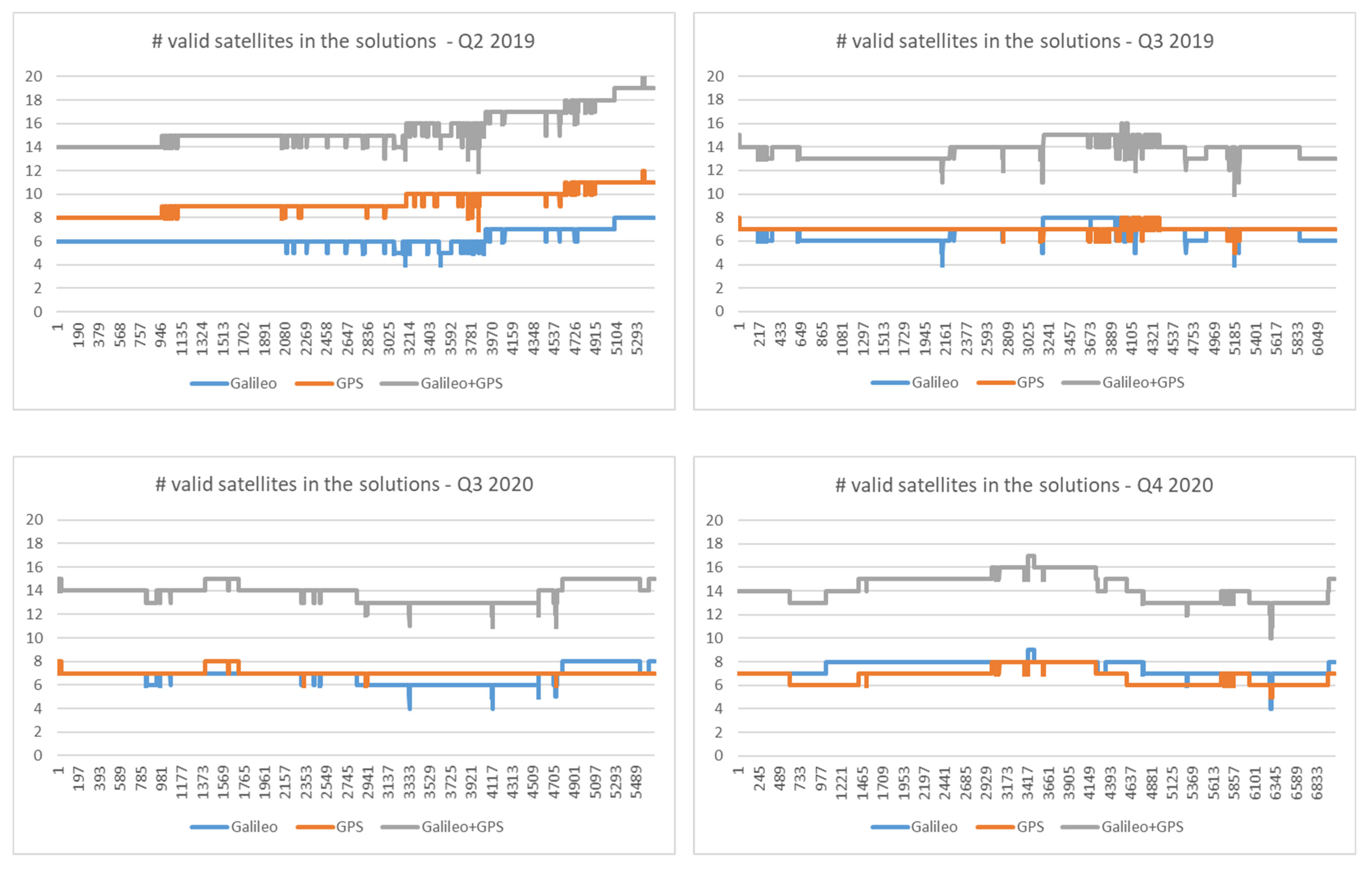
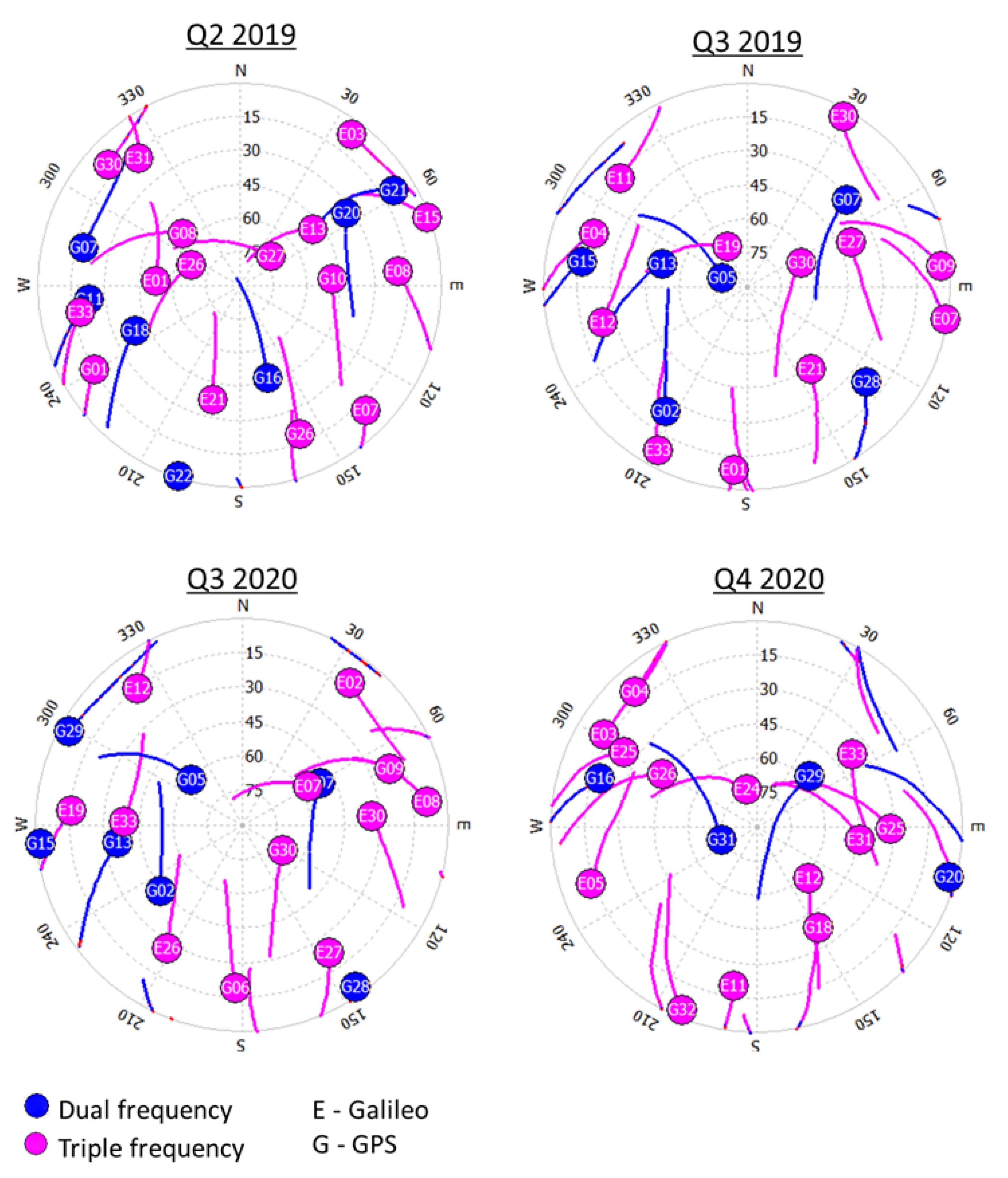
3.1. Results and Discussion for the Aerial Data-Collection Campaigns

Comparisons between the CSRS-PPP solutions and the differential triple-frequency (TF) solutions, based on code and carrier measurements, as well as the single-frequency code Single Point Positioning (SPP) solutions for the Galileo-only, GPS-only, and Galileo+GPS constellations [17] are presented in the figures below. For the Galileo+GPS solution, the GGTO (GPS to Galileo Time Offset) time offsets broadcasted in the navigation message were used.
As shown in the figures, the analysis was performed for the horizontal and vertical directions, and the provided results are the standard deviation and the mean values, all in meters.
Figure 8 provides the results of the comparison between the reference solutions and the triple-frequency differential solutions (GPS and Galileo) for the aerial campaigns.
From the figures above, we can see that, for the different aerial campaigns, the Triple-Frequency (TF) Galileo-only solutions are similar to the GPS-only and Galileo+GPS solutions. We can see standard deviation values varying between 1–11 cm for the horizontal component and 3–15 cm for the vertical component, respectively. In contrast, for the GPS-only solutions, the values are between 1–9 cm for the horizontal component and 3–17 cm for the vertical component. The combined Galileo+GPS solution shows values between 1–4 cm and 2–15 cm, respectively, for the horizontal and vertical components.
In terms of integer ambiguity fixing, the differential carrier phase solutions had a success rate near 99% for the different combinations, Galileo-only, GPS-only, and Galileo+GPS, in most of the campaigns.
Figure 9 shows the number of valid satellites used for the computation of differential carrier-phase solutions with RTKLib for Galileo-only, GPS-only, and Galileo+GPS, in each of the four campaigns.
It must be stressed that, in several campaigns, due to flight permission or meteorological constraints, the flights had to be conducted during periods with quite low satellite elevations. The most favorable situation, concerning satellite visibility and geometry, was during the June 2019 campaign (Q2 2019), as can be seen in Figure 10 and Figure 11. This might explain why, for the most recent campaigns, the Galileo-only and GPS-only results are not better than those of the older Q2 2019 campaign.
In the skyplots below, the fuchsia color indicates satellites with triple frequency, and the blue color indicates satellites with dual frequency (oldest GPS satellites). In the satellite elevation plots, the green and orange colors indicate satellites with SNR (Signal-to-Noise-Ratio) over 40 dBHz, which is what happens for most of the satellites above the 20° elevation.
Concerning the 95% confidence intervals, the values for Galileo-only data vary from 5 cm to 31 cm for the horizontal component and from 10 cm to 51 cm, for the vertical component. For GPS-only, the values vary between 2 cm and 30 cm for the horizontal and between 9 cm and 58 cm for the vertical components. For the combined Galileo+GPS solutions, the 95% confidence interval values vary between 2 cm and 12 cm for the horizontal and between 2 cm and 45 cm for the vertical components.
These results show that the quality of the Galileo-only results is identical to the GPS-only results and to the combined Galileo+GPS solutions. It should be noted that the number of Galileo satellites in the different campaigns was less than or equal to the number of GPS satellites, except for the Q4 2019 campaign.
When the DF results are compared with the GNSS/IMU or GPS/IMU (POS system) solutions, similar conclusions hold for the performance of the Galileo-only solution.
As referred to above, single-frequency SPP positions were also obtained for the different campaigns, and the results of these are shown in Figure 12 below. As for the differential solutions, in this case the CSRS-PPP solution was also used as a reference.
As we can see, Galileo-only SPP solutions have standard deviations not exceeding 0.3 m in the horizontal component and 0.8 m in the vertical component. For the GPS-only solution, the worst performance is observed, with values up to 1.1 m in the horizontal component and 2.6 m in the vertical component.
Concerning the 95% confidence intervals, the values for the Galileo-only SPP solutions are below 1.2 m and 4.2 m for the horizontal and vertical components, respectively.
The SPP Galileo-only results outperform both the GPS-only solution and the combined Galileo+GPS solution.
Table 8 indicates, for each campaign, the maximum number of satellites available during the observation time spans of around 1 h and 30 min and the corresponding average PDOP, for the Galileo, GPS and Galileo+GPS constellations.
The Galileo-only results presented above, both for TF differential and SF SPP, show the good performance of the Galileo system for kinematic airborne applications and standalone aerial navigation.
The SPP Galileo-only results, for the aerial campaigns, showed 95% confidence interval values, which are within the requirements for IFR (Instrument Flight Rules), as indicated in the European GNSS Agency (GSA) Market Report Issue 6, 2019 [29] (horizontal = 16 m, vertical = 4 m).

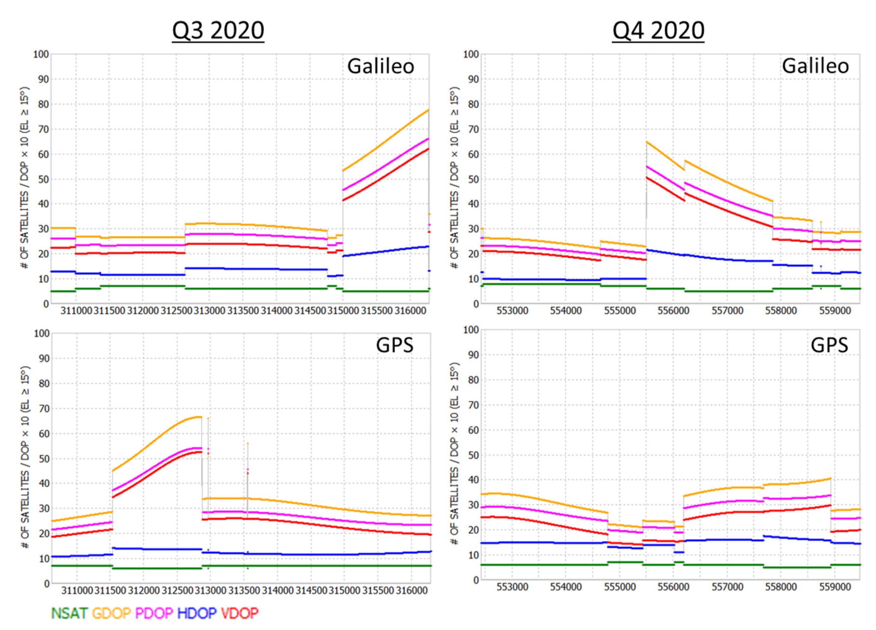
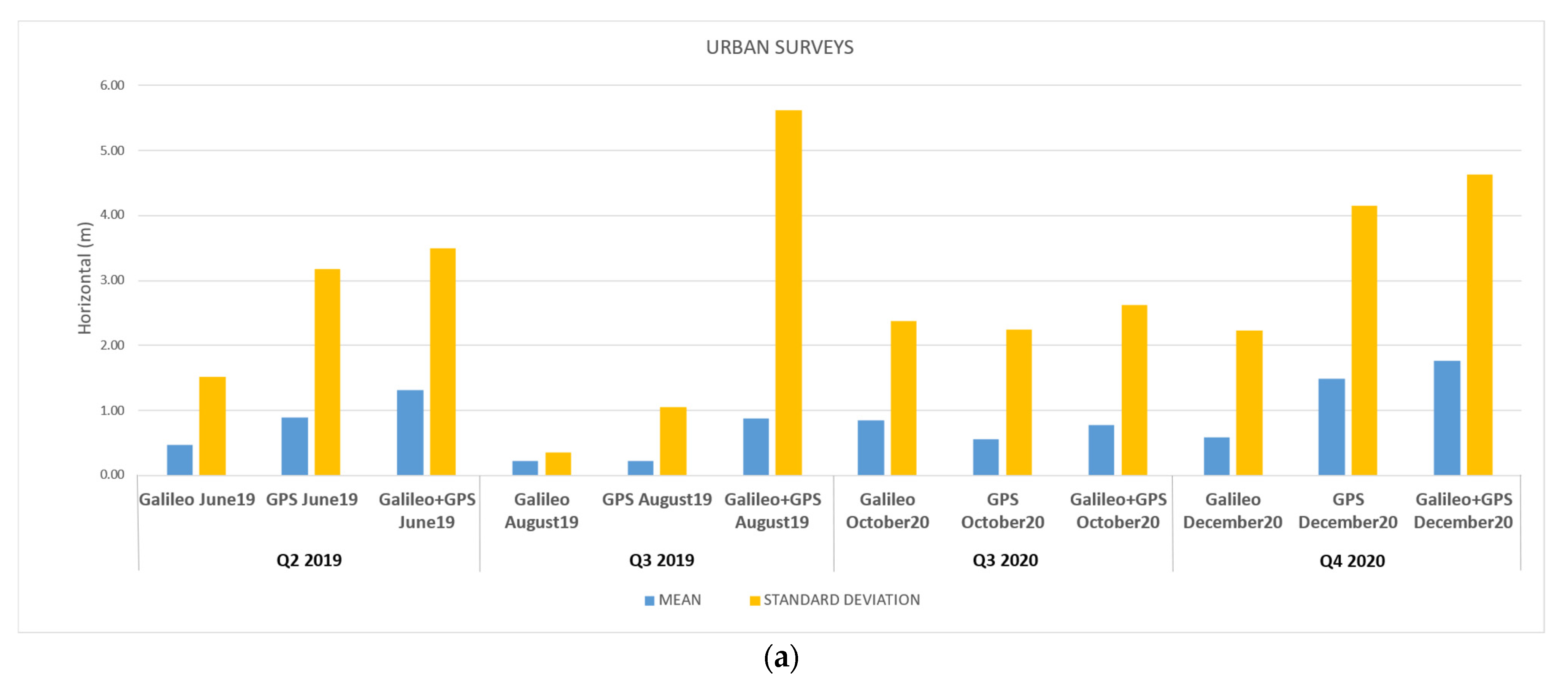
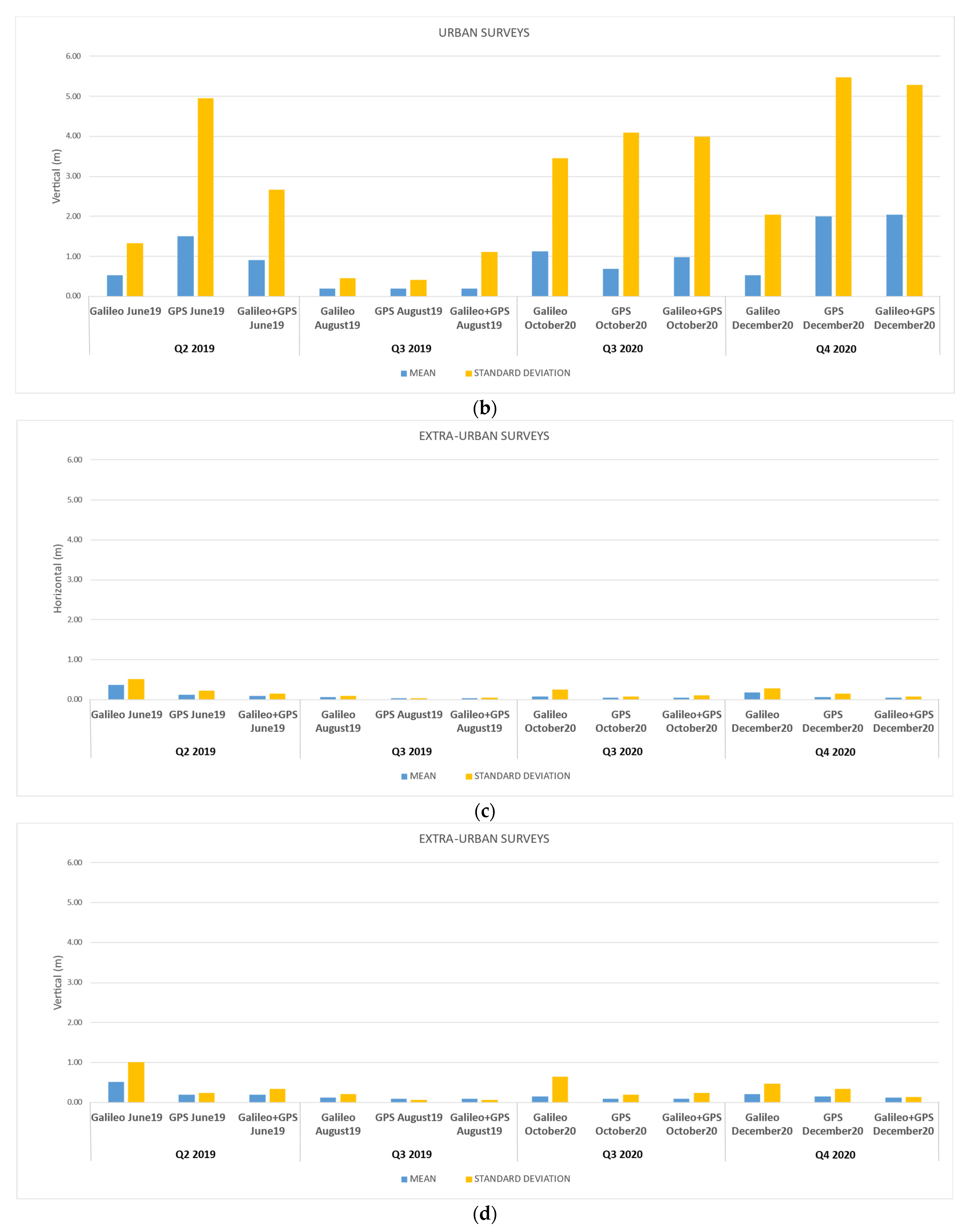
3.2. Results and Discussion for the Terrestrial Data-Collection Campaigns

Comparisons between the CSRS-PPP solutions and the differential post-processing DF solutions, for Galileo-only, GPS-only, and Galileo+GPS constellations were analyzed for the terrestrial campaigns. The analyses were performed for the horizontal and vertical directions for the urban and extra-urban surveys, and the provided results show the standard deviation and mean values in meters (Figure 13). Furthermore, the comparisons between the GNSS/INS solutions and the differential post-processing DF ones are given for Galileo-only, GPS-only, and Galileo+GPS constellations (Figure 14).
The results of the terrestrial urban campaigns revealed that Galileo-only solutions have lower standard deviation values than GPS in the August 2019 campaign and comparable values in the December 2020 campaign for the planimetric values; for the altimetric values, Galileo-only solutions provide better results than GPS in the June and August 2019 campaigns and comparable results in the December 2020 campaign.
The results of the extra-urban campaigns show that the Galileo means and standard deviations values aligned to the GPS ones, both for planimetric and altimetric values.
In general, the extra-urban surveys present higher accuracies than the urban ones. This is as expected, considering the RF (Radio Frequency) propagation environment features and the significant impact on satellite visibility and geometric configurations due to buildings and other obstacles (urban canyons).
Table 9 indicates the maximum numbers of satellites available and the PDOP averages for the Galileo-only, GPS-only, and Galileo+GPS constellations during each campaign (U: urban; E: extra-urban).
For the GNSS/IMU MMS comparisons, as far as regards the urban campaigns for GPS and Galileo data, improvements in the horizontal and vertical components between the campaign of June 2019 and August 2019 can be noticed. Regarding the October and December 2020 campaigns, the standard deviation values are higher with respect to the August 2019 campaign, both for the planimetric and altimetric components.
Apart from the October 2020 campaign, the Galileo standard deviation values for the horizontal component are lower than the GPS ones. The Galileo standard deviations for the vertical component are rather better than GPS deviations for the June 2019 and October and December 2020 campaigns. For the August 2019 campaign, they are comparable.
Regarding the extra-urban campaigns, the comparisons with the GNSS/INS MMS solutions show very good results, in particular since the August 2019 campaign, both for the horizontal and vertical components.
Starting from Q3 2019 campaign, the Galileo E1 E5b standard deviation values for the extra-urban surveys are lower than 0.28 m for the horizontal component and lower than 0.64 m for the vertical component. The horizontal values meet those required for a road-transportation domain according to the GSA Market Report Issue 6, 2019 [22], see Table 2.

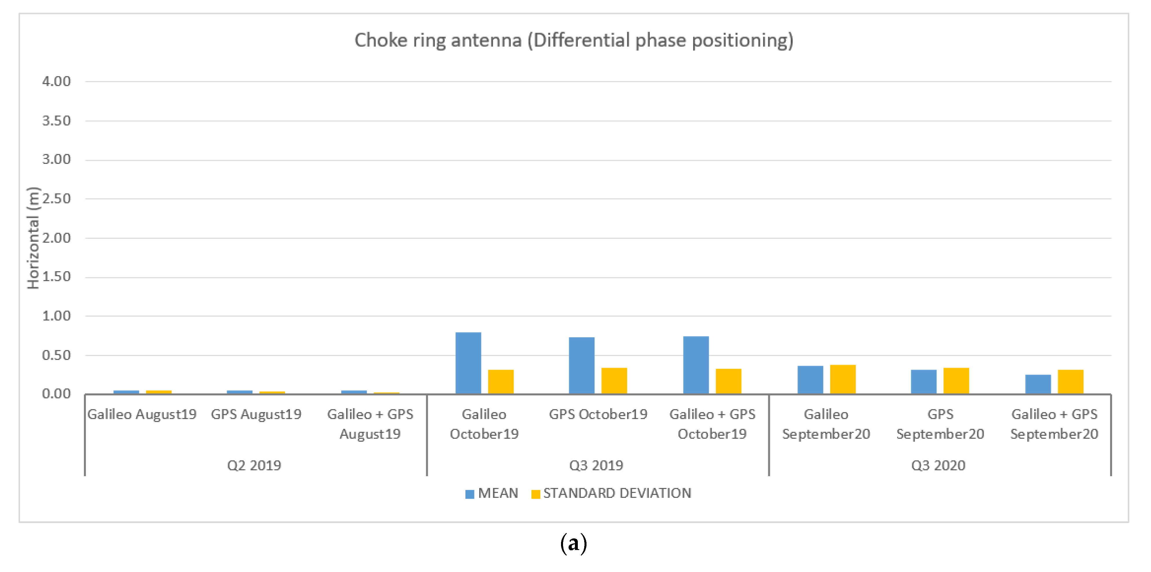
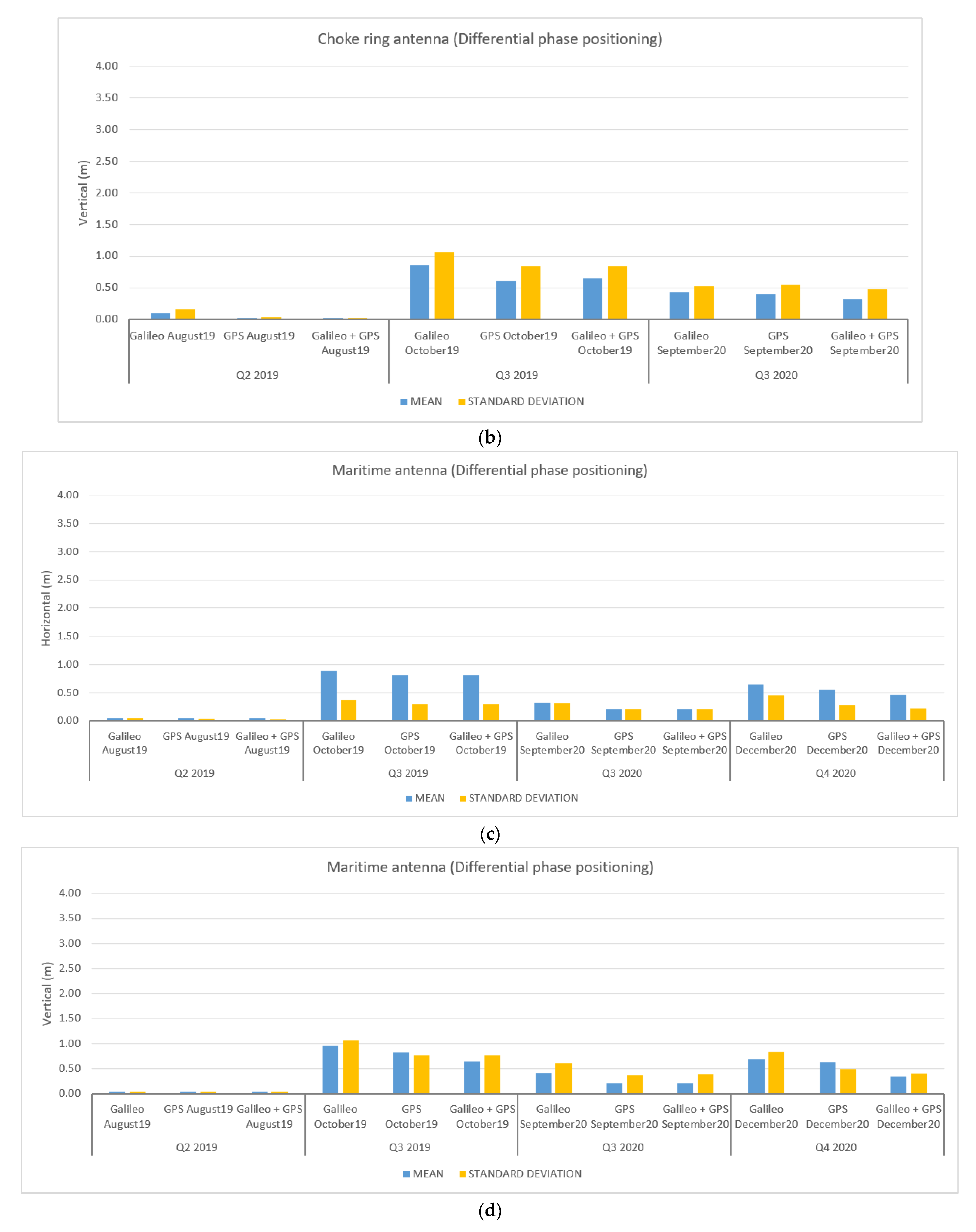
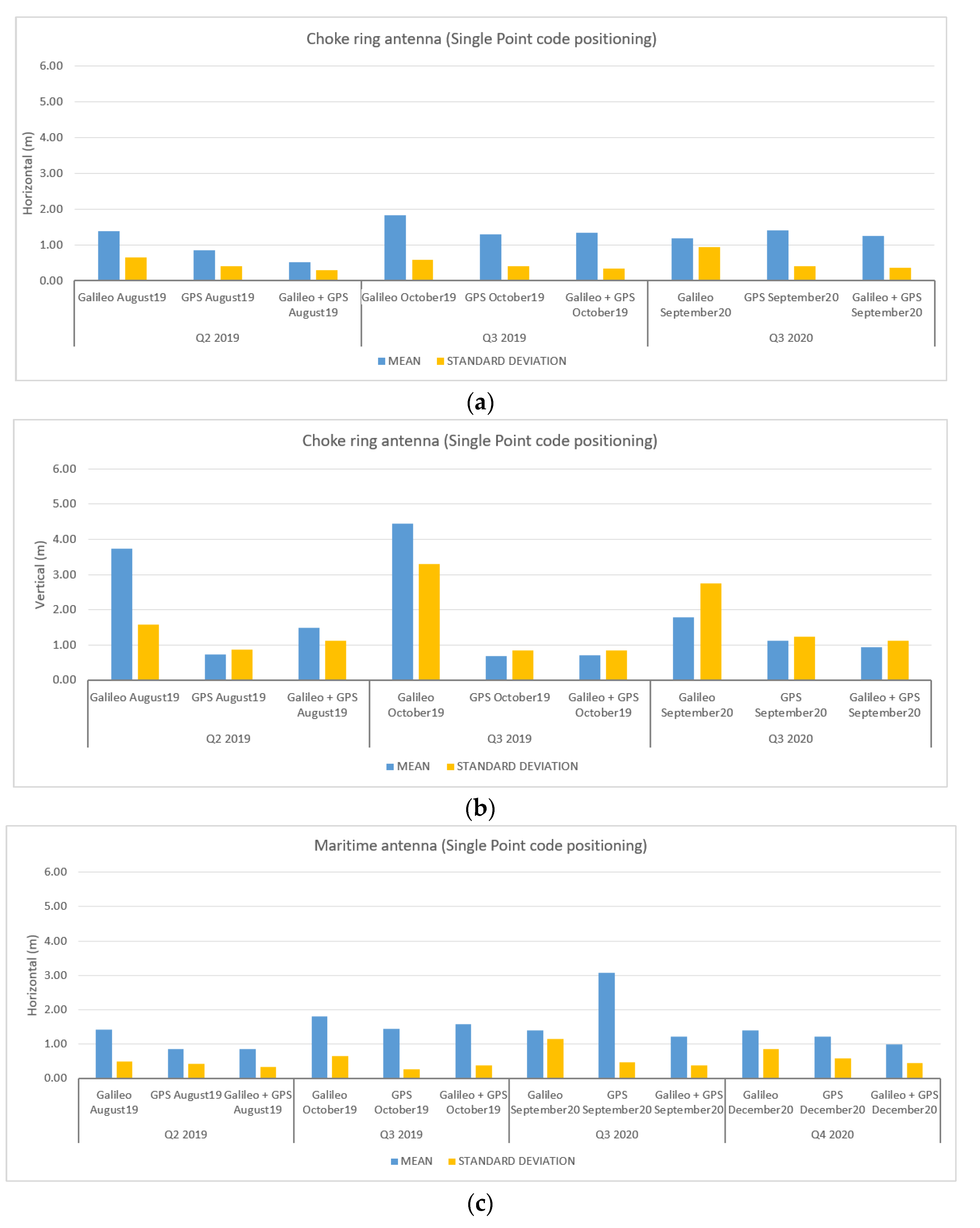
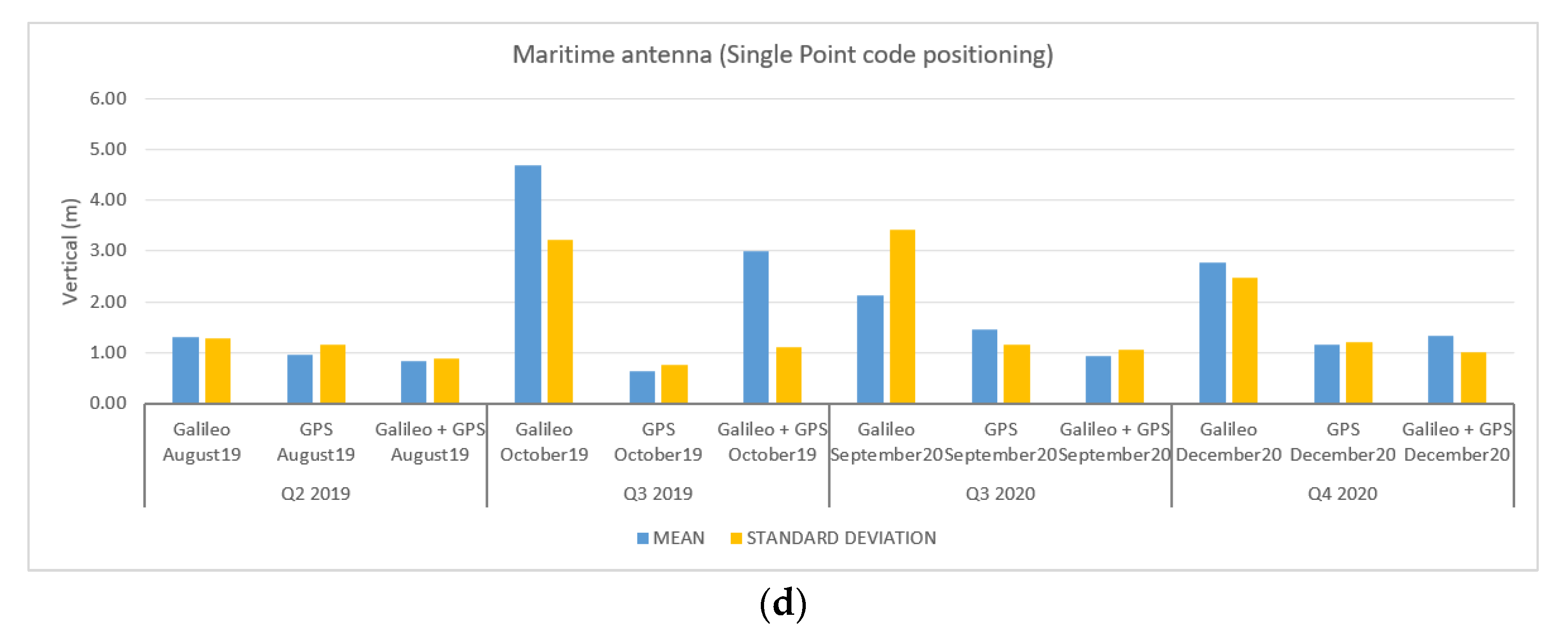
3.3. Results and Discussion for the Maritime Data-Collection Campaigns

As for the aerial data-collection campaign, comparisons between the CSRS-PPP reference solution and the differential triple frequency (TF) solutions, as well as the single point frequency code Single Point Positioning (SPP) solutions, Galileo-only, GPS-only, and Galileo+GPS constellations, are presented in the figures below. The analysis was performed for the horizontal and vertical directions, considering both the choke ring and the maritime antennas. The provided results are the standard deviation and mean values, all in meters.
Figure 15 presents the results of the comparison between the reference solution and the triple-frequency differential solutions (GPS and Galileo) for the two types of antennas.
Looking at the results from the different maritime campaigns, the standard deviations for the TF Galileo-only solutions have values between 4.5–45 cm for horizontal and between 4.5 cm–1 m for vertical components. When analyzing the results for the two types of antennas, the choke ring antenna has lower standard deviation results than the maritime antenna for the horizontal component, but the lowest vertical standard deviation is registered for the maritime antenna. For the GPS-only solutions, the values on the horizontal component are between 4–30 cm and, on the vertical component, between 4–84 cm. These solutions are similar for the two types of antennas, with lower maximum values for the maritime antenna type, both for the horizontal and vertical components. The combined Galileo+GPS solutions show values between 2.5–30 cm for the horizontal component and 3–84 cm for the vertical component. On both components, the lowest values for the standard deviation registered for the different types of solutions (Galileo-only, GPS-only, and Galileo+GPS) are similar, with a better similarity between the GPS and Galileo+GPS solutions. As for the two types of antennas, the maximum values of the standard deviation for each different type of solution were a few centimeters lower for the maritime antenna with respect to the choke ring antenna.
Concerning the mean values for the horizontal component, the Galileo-only solutions have values between 5 cm and 89 cm, with similar values for the GPS-only solutions (5 cm to 81 cm) and Galileo+GPS solutions. A similar situation is found for the vertical component, with slightly lower mean maximum values for the GPS-only and Galileo+GPS solutions.
A favorable context of more contributing factors led to good KPIs for all the differential solutions obtained in August 2019. From Figure 6, presenting the trajectories for each data-collection campaign, it can be observed that the August 2019 trajectory is in the port area, very close to the location of the GNSS reference station used for the differential phase approach. The short baseline between the GNSS base station and the kinematic trajectory is the first favorable factor. A second factor is represented by the PDOP values. In the case of Galileo, for August 2019, an average PDOP value of 3 was registered. This is the lowest average PDOP value registered from all the data-collection campaigns presented in this study. Another contribution factor is the satellite geometry. For the August 2019 data-collection campaign, three of the five available Galileo satellites had elevations higher than 55°. Another peculiarity of this data collection is that it had the highest number of epochs for all types of solutions compared to the other data-collection campaigns.
In terms of integer-ambiguity fixing, the differential carrier-phase solutions for the August 2019 data-collection campaign had a success rate higher than 97% for all the computed solutions. On the contrary, in December 2020, when the surveys were performed in the open sea at more than 100 km from the GNSS reference station, the success rate of the integer-ambiguity fixing for the kinematic solution was lower than 20%. A low integer-ambiguity-fixing rate of the differential carrier phase for the Galileo solution was also registered for the October 2019 data-collection campaign. For this campaign, unless the maximum number of visible Galileo satellites was 7 in the first hour of campaign, for more than 40 min, only 4 Galileo satellites were visible and had elevations lower than 45°, except one satellite.
Considering the above-mentioned factors and the fact that the number of GPS satellites was always higher (even double in some cases), from the comparison where we showed that the systems have similar residuals, the quality of the Galileo-only results can be highlighted. It is useful to mention again that, for the maritime data-collection campaign, only a PPP reference trajectory was computed, considering only GPS and GLONASS observations. This might also be a factor affecting the residual results for Galileo-only solutions.
Single-frequency SP positions were also obtained for the different campaigns, and the results are presented in Figure 16. As for the differential solution, the CSRS-PPP solution was used as a reference trajectory.
The standard deviation for the Galileo-only solutions has values lower than 1.1 m for the horizontal component and 3.4 m for the vertical component. For the GPS-only solutions, the horizontal component has values lower than 0.6 m, and the vertical has values lower than 1.2 m. As for the Galileo+GPS solutions, it has values lower than 0.4 m for the horizontal component and 1.1 m for the vertical component. For the maritime antenna, considering the two data-collection campaigns from 2020, an improvement can be observed both on the horizontal and vertical components for the September 2020 and December 2020 data-collection campaigns. Lower maximum-performance parameters were registered in the differential solutions for the maritime antenna, instead using the SPP approach; better values were registered in the horizontal component for the choke ring antenna. For the vertical component, no particular rule can be observed.
As for the mean values of the horizontal and vertical components, similar values are observed for the same solution (Galileo-only, GPS-only, Galileo+GPS) for both types of antennas. In terms of performance, the SPP Galileo-only solutions have lower performances compared to the GPS-only and Galileo+GPS. The Galileo+GPS solutions have the best values for the SPP approach.
Table 10 presents the maximum number of available satellites and the PDOP average values for each campaign for the Galileo-only, GPS-only, and Galileo+GPS constellations.
It can be observed that the Galileo-only solutions are characterized by the smallest number of satellites and the largest PDOP values out of all the campaigns. Analyses of the Galileo DOP values revealed the presence of several large jumps of at least 0.8 in each data-collection campaign. These jumps can be correlated to the decrease in the number of the available Galileo satellites tracked by the receiver. The GPS-only PDOP is much closer to the Galileo+GPS PDOP.
Considering all the results of the data-collection campaigns, in addition to the general factors (number of satellites, satellites geometry, PDOP, number of epochs) influencing the final results, the GNSS signals collected in the maritime environment can be influenced by factors such as the navigation environment (bridges, canyons, ports, etc.), the ship structure and antenna location, the sea state, and the ship’s movement. Looking at the DOP values for Galileo, the values were similar across the 2019 and 2020 data-collection campaigns.

4. Conclusions

This is probably one of the first projects where extensive Galileo airborne, terrestrial, and maritime kinematic data collection has been undertaken (12 campaigns were accomplished since the end of 2018, and more are foreseen until 2022), allowing a comprehensive analysis of Galileo and GNSS kinematic performances in various environments.
The results obtained in the different aerial campaigns allowed us to draw some conclusions about the actual system performance. In differential mode, the Galileo triple-frequency (TF) solutions showed standard deviations below 15 cm in both the horizontal and vertical components. In the SPP mode, the standard deviations are below 1 m for the horizontal and vertical components. Contrary to what was expected, the results for the 2021 campaign are not better that those obtained in the 2019 campaigns. This can be illustrated with a worst satellite geometry during part of the May 2021 flight campaign.
The results showed that the quality of the Galileo-only solutions is almost identical to that of the GPS-only or to the combined Galileo+GPS solutions.
If we keep in mind that the Galileo constellation is not yet fully complete and that the satellites’ visibility during some of the campaigns was not the best one (during several periods, satellites with quite low elevations had to be used in the computation of the solutions), we can already conclude that the Galileo system performs quite well and have the potential to fulfil the requirements for aerial navigation and to outperform GPS when satellite visibility is good.
As far as regards the terrestrial campaigns in general, the extra-urban surveys present higher accuracies than the urban ones. This is as expected, considering the significant impact on satellite visibility and geometric configurations due to the RF propagation environment (urban canyons). In the urban campaigns, the altimetric standard deviation values of the Galileo-only solutions are always lower than GPS values. For the extra-urban campaigns, the comparisons with the GNSS/IMU MMS solutions show very good results, in particular since the August 2019 campaign, for both the horizontal and vertical components.
Starting from the Q3 2019 campaign, the Galileo E1 E5b standard deviation values for the extra-urban surveys are lower than 0.28 m for the horizontal component and lower than 0.64 m for the vertical component. The horizontal values meet those required for the road-transportation domain.
The results obtained in the maritime campaigns show the high influence of the environment and of the number of satellites on the computation of the solutions. In differential mode, the Galileo-only solutions showed similar results to the GPS-only and Galileo+GPS solutions. Considering the comparison between the CSRS-PPP reference solution and the SPP solutions, the Galileo-only are lower than the GPS-only results; the Galileo+GPS solutions offer the best results. Based on the observed performance, the Galileo system fulfils the GNSS requirements for general navigation, as presented in [5]. Some constraints appear for the port navigation and restricted-waters navigation phases, where the accuracy ranges from 1 to 10 m. In differential mode, the Galileo-only maximum standard deviation of the positioning errors is 0.45 m, and, in SPP mode, it is 1.1 m. For SPP, this should be overcome with the evolution of the system and the increased number of satellites.
Across the different campaigns, the best results were obtained mainly by the Galileo+GPS combination, showing the good interoperability of Galileo and GPS. As for the Galileo-only system, the results obtained here show the consistent good performance of the Galileo system for all the different types of kinematic applications. Better performance of Galileo could be highlighted if we took into consideration the available number of satellites, PDOP values, and the geometry of both the Galileo and GPS systems.

Author Contributions

Conceptualization, R.C., A.R., L.B., P.B. and M.P.; methodology, R.C., A.R., L.B., M.P., P.B. and A.P.; data processing, P.S., R.C., T.S., A.I, A.R. and A.M.; validation, P.B. and M.P.; formal analysis, A.R., J.A.G., A.P., A.I., R.C., L.B., A.M., P.S. and T.S.; investigation, A.P., A.R., A.I., L.B., A.M., J.A.G., R.C., P.S. and T.S.; resources, A.R., A.P., R.C., L.B., M.P. and P.B.; data curation, A.R., L.B., R.C. and J.A.G.; writing—original draft preparation, R.C., A.R., A.I., A.P., L.B., M.P. and P.B.; writing—review and editing, R.C., A.R., L.B., M.P., P.B., A.I. and J.A.G.; visualization, A.R., A.P., A.I., R.C., L.B., J.A.G., P.B. and M.P.; supervision, R.C., A.R., L.B., M.P. and P.B.; project administration, A.R., L.B., J.A.G., R.C., M.P. and P.B.; funding acquisition, A.P., R.C. and L.B. All authors have read and agreed to the published version of the manuscript.

Funding

We acknowledge the European Union and the European Union Agency for the Space Programme (EUSPA) for supporting the cooperation of the Galileo Reference Centre (GRC) [27] with Member States within the GRC-MS project and co-financed (Grant agreement nr. GSA/GRANT/04/2016), in support of an independent monitoring of the Galileo system performance.

Conflicts of Interest

The authors declare no conflict of interest. The opinions expressed herein reflect the authors view only. The GRC-MS partners and EUSPA are not liable for the use of any of the information included herein.

References

  1. Someswar, G.M.; Rao, T.P.S.C.; Chigurukota, D.R. Global Navigation Satellite Systems and Their Applications. Int. J. Softw. Web Sci. 2013, 3, 17–23. [Google Scholar]
  2. Hall, E. History of the GNSS Industry and Milestones Ahead. GPS World. 2020. Available online: https://www.gpsworld.com/history-of-the-gnss-industry-and-milestones-ahead/ (accessed on 27 May 2022).
  3. Lavrov, A. Russia’s GLONASS Satellite Constellation. Moscow Defense Brief. 2017. Available online: http://cast.ru/products/articles/russia-s-glonass-satellite-constellation.html (accessed on 27 May 2022).
  4. BeiDou Navigation Satellite System. Available online: http://en.beidou.gov.cn/SYSTEMS/System/ (accessed on 19 April 2022).
  5. European Parliament and Council. Regulation (EU) No 1285/2013 of the European Parliament and of the Council of 11 December 2013 on the Implementation and Exploitation of European Satellite Navigation Systems. Off. J. Eur. Union 2013, 56, 1–32. [Google Scholar] [CrossRef]
  6. Tarantino, E.; Novelli, A.; Cefalo, R.; Sluga, T.; Tommasi, A. Single-Frequency Kinematic Performance Comparison between Galileo, GPS, and GLONASS Satellite Positioning Systems Using an MMS-Generated Trajectory as a Reference: Preliminary Results. ISPRS Int. J. Geo-Inf. 2018, 7, 122. [Google Scholar] [CrossRef] [Green Version]
  7. Odijk, D.; Teunissen, P.J.; Huisman, L. First results of mixed GPS + GIOVE single-frequency RTK in Australia. J. Spat. Sci. 2012, 57, 3–18. [Google Scholar] [CrossRef]
  8. Abd Rabbou, M.; El-Rabbany, A. Performance Analysis of GPS/GALILEO PPP Model for Static and Kinematic Applications. Geomatica 2015, 69, 75–81. [Google Scholar] [CrossRef]
  9. Rabbou, M.; El-Rabbany, A. Performance analysis of precise point positioning using multi-constellation GNSS: GPS, GLONASS, Galileo and BeiDou. Surv. Rev. 2017, 49, 39–50. [Google Scholar] [CrossRef]
  10. Liu, T.; Yuan, Y.; Zhang, B.; Wang, N.; Tan, B.; Chen, Y. Multi-GNSS precise point positioning (MGPPP) using raw observations. J. Geod. 2017, 91, 253–268. [Google Scholar] [CrossRef]
  11. Afifi, A.; El-Rabbany, A. Single Frequency GPS/Galileo Precise Point Positioning Using Un-Differenced and Between-Satellite Single Difference Measurements. Geomatica 2015, 68, 195–205. [Google Scholar] [CrossRef]
  12. Odolinski, R.; Teunissen, P.J.; Odijk, D. Combined BDS, Galileo, QZSS and GPS single-frequency RTK. GPS Solut. 2014, 19, 151–163. [Google Scholar] [CrossRef]
  13. Li, P.; Jiang, X.; Zhang, X.; Ge, M.; Schuh, H. GPS + Galileo + BeiDou precise point positioning with triple-frequency ambiguity resolution. GPS Solut. 2020, 24, 1–13. [Google Scholar] [CrossRef]
  14. Pan, L.; Zhang, X.; Liu, J. A comparison of three widely used GPS triple-frequency precise point positioning models. GPS Solut. 2019, 23, 121. [Google Scholar] [CrossRef]
  15. Rabbou, M.A.; Abdelazeem, M.; Morsy, S. Performance Evaluation of Triple-Frequency GPS/Galileo Techniques for Precise Static and Kinematic Applications. Sensors 2021, 21, 3396. [Google Scholar] [CrossRef] [PubMed]
  16. Song, J.; Zhao, L. Comparison Analysis on the Accuracy of Galileo PPP Using Different Frequency Combinations in Europe. Appl. Sci. 2021, 11, 10020. [Google Scholar] [CrossRef]
  17. Katsigianni, G.; Perosanz, F.; Loyer, S.; Gupta, M. Galileo millimeter-level kinematic precise point positioning with ambiguity resolution. Earth Planets Space 2019, 71, 76. [Google Scholar] [CrossRef] [Green Version]
  18. Krasuski, K.; Bakuła, M. Operation and reliability of an onboard GNSS receiver during an in-flight test. Sci. J. Sil. Univ. Technol. Ser. Transp. 2021, 111, 75–88. [Google Scholar] [CrossRef]
  19. Li, M.; Xu, T.; Flechtner, F.; Förste, C.; Lu, B.; He, K. Improving the Performance of Multi-GNSS (Global Navigation Satellite System) Ambiguity Fixing for Airborne Kinematic Positioning over Antarctica. Remote Sens. 2019, 11, 992. [Google Scholar] [CrossRef] [Green Version]
  20. Dautermann, T.; Korn, B.; Flaig, K.; de Haag, M.U. GNSS Double Differences Used as Beacon Landing System for Aircraft Instrument Approach. Int. J. Aeronaut. Space Sci. 2021, 22, 1455–1463. [Google Scholar] [CrossRef]
  21. Hinüber, E.L.V.; Reimer, C.; Schneider, T.; Stock, M. INS/GNSS Integration for Aerobatic Flight Applications and Aircraft Motion Surveying. Sensors 2017, 17, 941. [Google Scholar] [CrossRef] [Green Version]
  22. Elmezayen, A.; El-Rabbany, A. Real-Time GPS/Galileo Precise Point Positioning Using NAVCAST Real-Time Corrections. Positioning 2019, 10, 35–49. [Google Scholar] [CrossRef] [Green Version]
  23. Martin, S.; Kuhlen, H.; Schlotzer, S.; Schmitz-Peiffer, A.; Voithenberg, M.v.; Dietz, H. SEA GATE—A Maritime Galileo Testbed in the Port of Rostock. In Proceedings of the 20th International Technical Meeting of the Satellite Division of The Institute of Navigation (ION GNSS 2007), Fort Worth, TX, USA, 25–28 September 2007; pp. 535–542. [Google Scholar]
  24. Forschungshafen Rostock. Available online: https://www.forschungshafen.de/en/galileo-testbed-sea-gate/ (accessed on 27 May 2022).
  25. European GNSS Service Centre. Available online: https://www.gsc-europa.eu/sites/default/files/sites/all/files/Galileo_OS_SIS_ICD_v2.0.pdf (accessed on 27 May 2022).
  26. Marila, S.; Andrei, O.; Koivula, H.; Häkli, P.; Bilker-Koivula, M. GNSS Positioning Aspects for the Intelligent Shipping Test Laboratory at Rauma Harbor. In Proceedings of the International Conference on Localization and GNSS (ICL-GNSS 2020), Tampere, Finland, 2–4 June 2020. [Google Scholar]
  27. Buist, P.; Mozo, A.; Tork, H. Overview of the Galileo Reference Centre: Mission Architecture and Operational Concept. In Proceedings of the 30th International Technical Meeting of the Satellite Division of The Institute of Navigation (ION GNSS + 2017), Portland, OR, USA, 25–29 September 2017; pp. 1485–1495. [Google Scholar] [CrossRef]
  28. EUSPA. Available online: https://www.gsa.europa.eu/newsroom/news/galileo-reference-centre-now-officially-open (accessed on 27 May 2022).
  29. EUSPA. GSA Market Report Issue 6. 2019. Available online: https://www.gsa.europa.eu/gnss-market-report-issue-6-october-2019 (accessed on 27 May 2022).
  30. IMO (International Maritime Organization). Resolution, A.915(22), Adopted on 29 November 2001-Revised Maritime Policy and Requirements for a Future Global Navigation Satellite System (GNSS). Available online: https://wwwcdn.imo.org/localresources/en/KnowledgeCentre/IndexofIMOResolutions/AssemblyDocuments/A.915(22).pdf (accessed on 27 May 2022).
  31. Applanix Corporation. PUBS-MAN-001768-POSPacTM MMSTM GNSS-Inertial Tools Software Version 7.2, Revision 12-User Guide; Applanix Corporation: Richmond Hill, ON, Canada, 2016. [Google Scholar]
  32. Quan, W.; Li, J.; Gong, X.; Fang, J. INS/CNS/GNSS Integrated Navigation Technology; Springer: Berlin/Heidelberg, Germany, 2015; ISBN 978-3-662-45158-8. [Google Scholar]
  33. Cefalo, R.; Grandi, G.; Roberti, R.; Sluga, T. Extraction of Road Geometric Parameters from High Resolution Remote Sensing Images Validated by GNSS/INS Geodetic Techniques. In Proceedings of the Computational Science and Its Applications—ICCSA 2017, Trieste, Italy, 3–6 July 2017; Springer: Cham, Switzerland, 2017; Volume 10407, pp. 181–195. [Google Scholar] [CrossRef]
  34. Romanian Maritime Hydrographic Directorate Website. Available online: https://www.dhmfn.ro/en/catuneanu.shtml (accessed on 27 May 2022).
  35. IMO (International Maritime Organization). Resolution A.694(17), Adopted on 6 November 1991-General Requirements for Shipborne Radio Equipment Forming Part of the Global Maritime Distress and Safety System (GMDSS) and for Electronic Navigational AIDS. Available online: https://wwwcdn.imo.org/localresources/en/KnowledgeCentre/IndexofIMOResolutions/AssemblyDocuments/A.694(17).pdf (accessed on 27 May 2022).
  36. Canadian Spatial Reference System Precise Point Positioning (CSRS-PPP) Service. Available online: https://webapp.geod.nrcan.gc.ca/geod/tools-outils/ppp.php?locale=en (accessed on 27 May 2022).
  37. Takasu, T. RTKLIB: An Open Source Program Package for GNSS Positioning. Available online: http://www.rtklib.com/ (accessed on 27 May 2022).
  38. Klobuchar, J.A. Ionospheric Time-Delay Algorithm for Single-Frequency GPS Users. IEEE Trans. Aerosp. Electron. Syst. 1987, AES-23, 325–331. [Google Scholar] [CrossRef]
  39. Saastamoinen, J. Contributions to the theory of atmospheric refraction. Bull. Geod. 1973, 107, 13–34. [Google Scholar] [CrossRef]
  40. Petit, G.; Luzum, B. IERS Conventions. IERS Technical Note No. 36, 2010. Verlag des Bundesamts fur Kartographie und Geodasie, Frankfurt am Main. 2010. Available online: https://www.iers.org/IERS/EN/Publications/TechnicalNotes/tn36.html (accessed on 27 May 2022).
  41. Romanian Position Determination System. Available online: https://rompos.ro/ (accessed on 27 May 2022).
  42. EUREF Permanent GNSS Network. Available online: http://www.epncb.oma.be (accessed on 27 May 2020).
  43. Regione Autonoma Friuli-Venezia Giulia—Rete GNSS. Available online: http://www.regione.fvg.it/rafvg/cms/RAFVG/ambiente-territorio/conoscere-ambiente-territorio/FOGLIA1/ (accessed on 27 May 2022).
Figure 1. Countries in red have established a framework partnership agreement to support the GRC. Map generated in Esri®ArcMap™ 10.3. Used dataset: ESRI Data and Maps-World Countries (Generalized) dataset.
Remotesensing 14 03414 g001
Figure 2. Aircraft trajectories of the four aerial campaigns.
Remotesensing 14 03414 g002
Figure 3. Equipment used in the aerial data-collection campaigns. Left: Septentrio receiver, LN200 IMU and data logger; Middle: POS system; Right: AeroAntenna (foreground) and Sensor Systems antenna (background) fixed on the aircraft.
Remotesensing 14 03414 g003
Figure 4. The surveyed area for terrestrial data collection. (a) in green, the reference trajectory produced by the Mobile Mapping System Position and Orientation System for Land Vehicles (MMS POS/LV system) in the urban experiment. (b) in red, the extra-urban survey.
Remotesensing 14 03414 g004
Figure 5. The MMS of the GeoSNav Lab, University of Trieste, and the Applanix Corporation POS/LV© system components mounted on board the vehicle. MMS data were used to create the reference trajectory.
Remotesensing 14 03414 g005
Figure 6. Trajectories of the maritime campaigns. Reference GNSS station is situated in the Port of Constanta on the Black Sea.
Remotesensing 14 03414 g006
Figure 7. Experimental setup for the maritime data-collection campaign. (a) the GNSS antennas installed on the bow lighting mast of the Catuneanu vessel; (b) the special rack containing the GNSS receivers and the external power supply.
Remotesensing 14 03414 g007
Figure 8. Horizontal (a) and vertical (b) mean values and standard deviations (in meters) for the triple-frequency differential solutions in the different aerial campaigns using CSRS-PPP as reference.
Remotesensing 14 03414 g008
Figure 9. Number of valid satellites used in the aerial solutions estimations.
Remotesensing 14 03414 g009
Figure 10. Skyplots for Galileo and GPS during the four aerial campaigns.
Remotesensing 14 03414 g010
Figure 11. Satellite geometry for Galileo and GPS during the aerial four campaigns (values ×10). The green line indicates the total number of satellites in view.
Remotesensing 14 03414 g011aRemotesensing 14 03414 g011b
Figure 12. Horizontal (a) and vertical (b) mean values and standard deviations (in meters) for the SPP code solutions in the different campaigns using CSRS-PPP as reference.
Remotesensing 14 03414 g012
Figure 13. Horizontal and vertical mean values and standard deviations (in meters) for the different campaigns in terrestrial environments (urban and extra-urban) using CSRS-PPP as reference (a,b) for urban and (c,d) for extra-urban surveys.
Remotesensing 14 03414 g013aRemotesensing 14 03414 g013b
Figure 14. Horizontal and vertical mean values and standard deviations (in meters) for the different campaigns in terrestrial environments (urban and extra-urban) using GNSS/INS MMS as reference: (a,b) for urban, (c,d) for extra-urban surveys.
Remotesensing 14 03414 g014aRemotesensing 14 03414 g014b
Figure 15. Horizontal and vertical mean values and standard deviations (in meters) for the different campaigns in maritime environments, using CSRS-PPP as reference and the triple frequency differential solutions: (a) horizontal and (b) vertical for the choke ring antenna; (c) horizontal and (d) vertical for the maritime antenna.
Remotesensing 14 03414 g015aRemotesensing 14 03414 g015b
Figure 16. Horizontal and vertical mean values and standard deviations (in meters) for the SPP code solutions in maritime environments, using CSRS-PPP as reference for: (a) horizontal and (b) vertical for the choke ring antenna; (c) horizontal and (d) vertical for the maritime antenna.
Remotesensing 14 03414 g016aRemotesensing 14 03414 g016b
Table 1. Key requirements for the aeronautics domain.
ApplicationsNon-Safety Navigation (Relevant for General Aviation Visual Flight Rules (VFR))Performance Based Navigation (Relevant for all Instrument Flight Rules (IFR))Surveillance (Including ADS-B)
Key GNSS requirementsAvailabilityAccuracy (16 m horizontally, 4 m vertically for 95% of the time),
Availability (99–99.999%),
Continuity,
Integrity
Robustness
Accuracy,
Availability,
Integrity,
Robustness
Table 2. High priority requirements for the road transportation domain.
ApplicationsSafety Related Automatic
Actions in V2X, Autonomous
Driving, eCall, Tracking and Tracing
of Dangerous Goods
Liability: RUC,
Pay-as-you-Drive,
Taxi Meter,
Smart Tachograph
Smart Mobility: Road Navigation
Automated Parking
Dynamic Ride Sharing
Key GNSS requirementsAccuracy
(decimeter-level)
Authentication
Availability (>99.5%)
Integrity
Robustness
TTFF
Accuracy
(decimeter-level)
Authentication
Availability (>99.5%)
Integrity
Robustness
TTFF
Authentication
Integrity
Other requirementsConnectivity (mainly short range)
Interoperability
Connectivity (short range and long range)Connectivity (long range)
Table 3. High priority requirements for the maritime domain.
ApplicationsNavigation 1Ship OperationsTraffic Management and TrackingSearch and RescuePort OperationsEngineering and Offshore
Key GNSS requirementsAccuracy (from meter to 10 m)Accuracy
(from sub-meter to 10 m)
AvailabilityAccuracy
(final approach 5 m)
Accuracy
(sub-meter)
Accuracy (sub-meter)
Availability
AvailabilityAvailabilityContinuityAvailabilityAvailabilityIntegrity
IntegrityIntegrity IntegrityTIFF
1 The GNSS requirements for general navigation vary with the given maritime environment.
Table 4. Data-collection campaigns.
QuarterData-Collection TypeDateApproximate DurationPVT Solution
Computation Technique
Reference Trajectory
Computation Method
Q2 2019Aeronautical5 June 20191.5 hTF 1 (phase differential)
SF 2 (phase differential)GPS/IMU 4 (differential)
SPP 3 (code only)PPP 5
Terrestrial (urban)3 June 20191 hDF 6 (phase differential)GNSS/IMU (differential)
PPP
Terrestrial (extra-urban)3 June 20191.2 hDF (phase differential)GNSS/IMU (differential)
PPP
Maritime16 August 20192 hTF (phase differential)
SPP (code only)
PPP
Q3 2019Aeronautical7 October 20191.7 hTF (phase differential)
SF (phase differential)GPS/IMU (differential)
SPP (code only)PPP
Terrestrial (urban)6 August 20191 hDF (phase differential)GNSS/IMU (differential)
PPP
Terrestrial (extra-urban)6 August 20191.2 hDF (phase differential)GNSS/IMU (differential)
PPP
Maritime2 October 20192 hTF (phase differential)
SPP (code only)
PPP
Q3 2020Aeronautical7 October 20191.5 hTF (phase differential)
SF (phase differential)GPS/IMU (differential)
SPP (code only)PPP
Terrestrial (urban)27 October 20201.2 hDF (phase differential)GNSS/IMU (differential)
PPP
Terrestrial (extra-urban)27 October 20201.2 hDF (phase differential)GNSS/IMU (differential)
PPP
Maritime8 September 20202 hTF (phase differential)
SPP (code only)
PPP
Q4 2020 7Aeronautical8 May 20212 hTF (phase differential)
SF (phase differential)GPS/IMU (differential)
SPP (code only)PPP
Terrestrial (urban)18 December 20201.4 hDF (phase differential)GNSS/IMU (differential)
PPP
Terrestrial (extra-urban)18 December 20201.3 hDF (phase differential)GNSS/IMU (differential)
PPP
Maritime17 December 20202 hTF (phase differential)
SPP (code only)
PPP
1 TF: triple-frequency; 2 SF: single-frequency; 3 SPP: Single-Point Positioning; 4 IMU: Inertial Measurement Unit; 5 PPP: Precise-Point Positioning; 6 DF: Dual-frequency; 7 Due to the lockdown in Portugal (COVID-19), the Q4 2020 campaign had to be postponed until May 2021.
Table 5. Equipment used in the aerial data-collection campaigns.
EquipmentDescription
1 × Litton LN-200 (Northrop Grumman, Falls Church, VA, USA)FOG Inertial Measurement Unit (IMU)
1 × FCUP datalogger (FCUP, Porto, Portugal)LN200 datalogger with 1PPS from GPS
1 × AEROcontrol POS system (IGI mbH, Kreuztal, Germany)GPS/IMU system (Novatel OEM4/OEMV GPS L1/L2 receiver + FOG IMU)—airplane own system
1 × GPS L1/L2 Antenna (Sensor Systems Inc., Chatsworth, CA, USA)GPS antenna S67-1575-96
1 × Septentrio PolaRx5 (Septentrio, Leuven, Belgium)Multi-constellation GNSS receiver
1 × GNSS Antenna (AeroAntenna Technology Inc., Chatsworth, CA, USA)AT1675-381_B AA TSO ANT MF L
1 × 12 V 14 Ah valve regulated lead–acid battery (Shimastu, Tsuen Wan NT, Hong Kong)LN200 power supply
1 × 12 V 14 Ah valve regulated lead–acid battery ((Shimastu, Tsuen Wan NT, Hong Kong)Septentrio receiver power supply
Table 6. Equipment used in the terrestrial data-collection campaigns.
EquipmentDescription
1 × Litton LN-200 (Northrop Grumman, Falls Church, VA, USA)Inertial system
1 × Hercules encoder H35T-142P-FU1024 (Hercules, WI, USA)Odometer
2 × Trimble (Trimble, Sunnyvale, CA, USA)GPS receiver
2 × Trimble Zephyr (Trimble, Sunnyvale, CA, USA)GPS antenna
1 × Septentrio AsteRx-U (Septentrio, Leuven, Belgium)Multi-constellation GNSS receiver
1 × Septentrio PolaNT-X MF (Septentrio, Leuven, Belgium)GNSS antenna
1 × 12 V 15,600 mAh power supply (XTPower, China)Septentrio receiver power supply
1 × 12 V 60 Ah Lead-acid battery (Varta, Hannover, Germany)Applanix POS/LV power supply
Table 7. Equipment used in the maritime data-collection campaigns.
EquipmentDescription
1 × Advantech UNO-3283G (Advantech, Taipei, Taiwan)Computer
2 × AsteRx-U (Septentrio, Leuven, Belgium)Multi-constellation, dual antenna GNSS receiver
2 × 12 V 6 Ah Power supply (Mean Well Enterprises Co., LTD., New Taipei City, Taiwan)Power supply
2 × 12 V 2 Ah Lead-acid battery (GS YUASA Battery Germany GmbH, Krefeld, Germany)Power backup
1 × PolaNt Choke Ring B3/E6 * (Septentrio, Leuven, Belgium)GNSS antenna
2 × PolaNt-x MF ** (Septentrio, Leuven, Belgium)GNSS antenna
* In the Q4 2020 data-collection campaign, due to the addition of new equipment on the host ship (not belonging to our project), the PolaNt-x Choke Ring antenna was no longer used, only the PolaNt-x MF antenna. ** The experimental setup on board the ship included two PolaNt-x MF antennas (as can be seen in Figure 7), but one of them was used as secondary antenna, and the data collected by the receiver connected to this antenna were not used for the analysis.
Table 8. Average PDOP and maximum satellites number during the aerial data-collection campaigns.
GalileoGPSGalileo+GPS
CampaignPDOPNo SVPDOPNo SVPDOPNo SV
Q2 20191.5111.5130.923
Q3 20191.8101.610119
Q3 20201.891.69118
Q4 20201.5101.49119
Table 9. Average PDOP and maximum satellites number during the terrestrial data-collection campaigns.
GalileoGPSGalileo+GPS
CampaignPDOPNo SVPDOPNo SVPDOPNo SV
UEUEUEUEUEUE
Q2 20192.423.55653.212.158112.391.681416
Q3 20192.732.93562.211.6211112.081.281616
Q3 20203.192.19662.671.95992.371.281515
Q4 20202.312.23662.882.35882.361.471414
Table 10. Average PDOP and maximum number of satellites during the maritime data-collection campaigns.
GalileoGPSGalileo+GPS
CampaignPDOPNo SVPDOPNo SVPDOPNo SV
Q2 2019352.181.513
Q3 20194.571.9101.416
Q3 20203.261.9101.316
Q4 20204.461.7111.417
Publisher’s Note: MDPI stays neutral with regard to jurisdictional claims in published maps and institutional affiliations.

