Abstract
Microseismic monitoring is a useful enabler for reservoir characterization without which the information on the effects of reservoir operations such as hydraulic fracturing, enhanced oil recovery, carbon dioxide, or natural gas geological storage would be obscured. This research provides a new breakthrough in the tracking of the reservoir fracture network and characterization by detecting the microseismic events and locating their sources in real-time during reservoir operations. The monitoring was conducted using fiber optic distributed acoustic sensors (DAS) and the data were analyzed by deep learning. The use of DAS for microseismic monitoring is a game changer due to its excellent temporal and spatial resolution as well as cost-effectiveness. The deep learning approach is well-suited to dealing in real-time with the large amounts of data recorded by DAS equipment due to its computational speed. Two convolutional neural network based models were evaluated and the best one was used to detect and locate microseismic events from the DAS recorded field microseismic data from the FORGE project in Milford, United States. The results indicate the capability of deep neural networks to simultaneously detect and locate microseismic events from the raw DAS measurements. The results showed a small percentage error. In addition to the high spatial and temporal resolution, fiber optic cables are durable and can be installed permanently in the field and be used for decades. They are also resistant to high pressure, can withstand considerably high temperature, and therefore can be used even during field operations such as a flooding or hydraulic fracture stimulation. Deep neural networks are very robust; need minimum data pre-processing, can handle large volumes of data, and are able to perform multiple computations in a time- and cost-effective way. Once trained, the network can be easily adopted to new conditions through transfer learning.
1. Introduction
The global energy demand is projected to increase. To meet the increasing energy demand requires new technologies to exploit unconventional reserves. Similarly, calls for climate actions such as carbon geosequestration, hydrogen generation, and geological hydrogen storage will require an improvement in reservoir characterization methods [1,2,3,4]. Seismology remains one of the most relevant instruments in reservoir characterization. The importance of seismology in reservoir characterization is extensively covered in the literature [5,6,7,8,9]. Similarly, the application of microseismic monitoring is well documented in the literature [10].
1.1. Microseismology in Reservoir Characterization
Estimating the petrophysical properties of reservoirs is integral to reserve and resource estimation. While petrophysical measurements from well logs adequately evaluate the reservoir properties, the correlation with seismic data better validates the measured properties and reduces errors [11,12]. The availability of continuous microseismic data helps us to understand the geomechanical and petrophysical changes in the reservoir. Furthermore, the real-time data and analysis of such petrophysical changes could contribute to the initial screening process of feasible enhanced oil recovery methods [13].
Hydraulic fracturing is one of the most popular techniques for enhanced oil recovery and geothermal production. It involves the injection of huge volumes of a special liquid under high pressure into the geological formations to create new fractures and open up existing ones. Since this process has a direct mechanical effect on the geological formations, there is a potential to induce microseismic events locally. Foulger [14] indicated that about 21 earthquakes were induced due to hydraulic fracturing. Similar geological exploitation such as geothermal energy extraction has also been reported to have an increased microseismic rate [15,16].
Numerous processes involving the injection of gases have been at the forefront of studies in recent years. While the techniques of injecting CO2 into geological formations are well advanced, the assurance of the safety of the storage sites for many years to come remains an unanswered question. The storage of CO2 presents potential changes in the physical, chemical, and mechanical state of the geological formations and in situ reservoir brine [17,18,19,20,21]. An example was demonstrated in the study by Oye et al. [22], who showed the occurrence of microseismic events in clusters within a limited spatial area, which was attributed to CO2 injection. Hydrogen gas requires higher storage volumes due to its low volume to burn ratio [23]. One of the proposed storage solutions for hydrogen for future use is its storage in geological formations [24,25]. The concern of this storage mechanism is the possible induction of microseismic events due to pressure build-up as well as the loss of hydrogen in the geological formation [26]. Similar concerns have been attributed to the underground storage of gas [27].
At the end of the life cycle of a well, a well abandonment and decommissioning operation is implemented to isolate and prevent the further inflow of hydrocarbons or the migration of hydrocarbons upward, which could contaminate the upper layer water-bearing zones. However, while the techniques implored in well plugging and abandonment are well advanced, the longevity of the integrity of the well is difficult to predict. Hence in most cases, there is a need for the continuous monitoring of wellbore integrity and other previously induced microseismic events [28,29].
1.2. DAS in Reservoir Characterization
For a long time, three-dimensional vertical seismic profiling (3D-VSP) has been considered as appealing for imaging complex subsurface structures, both in exploration and time-lapse monitoring for the characterization of reservoirs. However, the associated costs and complexity of installing geophone arrays in a well as well as the scarcity of available wells have hampered the widespread deployment of 3D-VSP [30]. These challenges can essentially be reduced by the use of the novel distributed acoustic sensing (DAS) technology.
DAS uses an ordinary or engineered fiber optic cable for seismic monitoring. In its deployment, an interrogation unit (IU) is attached at the end of the fiber optic cable near or on the surface. The IU measures the deformations (contractions or extensions) along the fiber optic cable caused by propagating seismic waves. This sort of measurement is known as distributed acoustic sensing. “Distributed” because any part of the fiber cable can be deformed and logged for seismic information.
DAS measurements are straightforward in concept. A laser pulse is sent down the fiber cable by the IU. As the pulse propagates through the cable, portions of it undergo Rayleigh back-scattering due to the minute heterogeneities in the cable. When a seismic wave interacts with the cable, deforming it, it causes changes in the patterns of the back-scattered light, which is then converted into seismic data. The time it takes the back-scattered pulse to travel back to the IU allows for an accurate location of the point of deformation. Due to the fast speed of light, the entire length of the fiber optic cable can be interrogated with laser pulses at frequencies far greater than those of seismic waves. Depending on the length of the borehole, the interrogation frequencies typically range from 10 to 100 kHz, with higher frequencies known to produce a higher signal-to-noise ratio (SNR) due to redundancy. Nonetheless, the length of the borehole restricts the highest permissible frequency.
The first demonstration of the capability of use of DAS for VSP acquisition was by Mestayer et al. [31]. There has since been tremendous progress in the development and testing of DAS technology that has resulted in its almost unrivalled acceptance for a wide range of field seismic measurements. In relation to reservoir characterization, DAS has been applied to microseismic monitoring and analysis [32,33,34], hydraulic fracture monitoring [35,36] as well as in flow and production monitoring [37,38,39].
1.3. Deep Learning
Deep learning [40] is a branch of machine learning that has gained traction in the field of seismic data processing, analysis, and interpretation due to its computational efficiency, adaptability, and inherent ability to extract high-level features from recorded seismic waveforms with little to no manual engineering. Developed for pattern recognition in computer vision, deep learning models have high-level feature extraction mechanisms that enable them to transform raw data into a subset of feature vectors, allowing learning to take place. This makes them a perfect candidate for classification or regression tasks. The detection of seismic events is a classic example of a classification task, while inversion to locate the origin of the seismic energy can be considered as a multidimensional regression problem. The most popular deep learning architectures in seismology are recurrent neural networks (RNNs) and convolutional neural networks (CNNs). The latter is preferred for its processing speed and ability to handle large volumes of data; the former’s ability to recognize sequential patterns in the data and use those patterns to predict the next possible scenario makes it the de facto time series analysis tool.
Because deep learning models are data-driven, they require a significant amount of data for training and validation. As a result, they are best suited to processing seismic data recorded by the DAS, which collects massive amounts of data. Binder and Tura [41] employed convolutional neural networks to automatically detect microseismic events in the data acquired by DAS along a borehole during a hydraulic fracture operation. They compared the results with those from a surface geophone array and observed that, despite the low SNR in the DAS data, the neural network was able to detect 167 new events that were not registered by the geophones. Huot et al. [42] reported a 98.6% accuracy of deep learning models trained with hyperparameters obtained by Bayesian optimization on 7000 manually selected microseismic DAS events. They concluded that by the application of AI, the model was able to predict more than 100,000 events, which enhanced the prediction of the spatio-temporal fracture developments, which otherwise could not have been detected by traditional methods. Furthermore, to overcome the problem of SNR that makes the data processing challenging, Qu et al. [43] introduced a new methodology based on fixed segmentation coupled with a support vector machine (SVM) model. The proposed methodology allowed for the identification of the best features and the optimal number of features required for producing accurate results. From the comparative analysis, the presented model had accurate results compared to the CNN and the short-term average and long-term average ratio (STA/LTA) conventional approach. Other applications of deep learning for the detection of seismic/microseismic activities are well-documented in [44,45,46,47].
Deep learning has also been applied to tasks other than the detection and classification of seismic activities. Wamriew et al. [48] demonstrated the potential application of deep learning to the inversion of microseismic data. They showed that a CNN model was capable of locating microseismic events and reconstructing the velocity model simultaneously in real-time from seismic waveforms. Tanaka et al. [49] employed a deep learning model to perform moment tensor inversion of acoustic emissions during a hydraulic fracturing experiment of granite rock and obtained 54,727 solutions.
Due to their computational efficiency, the models can be used in the field to process the data in real-time during its acquisition, thereby scaling down the amount of data to be stored while providing necessary information that could help optimize the field operations. Huot and Biondi [50], Wamriew et al. [51], and Huot et al. [52] emphasized that without the complete automation of microseismic data processing, large volumes of collected data could be wasted due to human processing limitations.
It is well-established in the literature that the active and real-time recording and processing of microseismic activities is very essential for the characterization of geological formations. Right from the exploration of the field to the appraisal, the development, production, enhanced, and improved oil recovery methods, abandonment well monitoring or utilization for the storage of CO2 or H2. In addition, the challenges of the physical processing of huge volumes of microseismic data and the limitations imposed could be overcome by the implementation of automated artificial intelligence models, as have been developed in recent times that could predict events and analyze the geological changes in reservoirs. In this study, we demonstrate the use of two cutting-edge technologies: distributed acoustic sensing (DAS) and deep learning for microseismic monitoring and analysis. Building on the work by Wamriew et al. [51], we investigated the possibility of improved microseismic event detectability and location: (i) given a well-known velocity model; (ii) using different neural network architectures; and (iii) reducing the number of output parameters. In addition, the output detections by the neural networks were verified using the conventional STA/LTA method.
2. Materials and Methods
2.1. Microseismic Data
The process of obtaining a high-resolution DAS microseismic dataset requires the use of specific data processing. This is mainly due to the technological features of the data acquisition. In the most typical downhole DAS installation, the fiber optic cable is permanently cemented on the outside of the well-casing. When a propagating seismic wavefield from a source passes through the fiber optic cable, it reacts to the propagation and, as a result, lengthens and shortens in the longitudinal direction of the fiber optic cable. The lengthening and shortening of the fiber optic cable cause interference wave patterns, similar to the vibrations of a coil in a conventional survey seismic receiver. These interference patterns are collected and interpreted by the interrogation unit, which reproduces the seismic waveform at specific points on the cable. Usually these points are arranged in constant increments every 1–5 m, similar to a receiver array. The distance between the “receivers” in the DAS cable results in the revolutionary ability of the DAS cable to provide inexpensive, high spatial, and temporal resolution downhole seismic measurements.
In this study, we used the downhole DAS microseismic data recorded during the phase 2C hydraulic fracture stimulation experiment at the FORGE research site near Utah, in the United States. These data are available in the public domain [53,54,55]. The data were acquired in a 1000 m deep vertical monitoring well installed with a Silixa Carina® Sensing iDAS system that natively measures the strain-rate. This monitoring well was situated 400 m to the southeast of the treatment well from which the hydraulic fracturing stimulation experiments were conducted over the period 14 April 2019 to 3 May 2019 [54]. The data were recorded with a channel spacing of 1 m, gauge length of 10 m, and at a frequency of 2000 Hz.
The complete dataset was comprised of 40 detected microseismic events with moment magnitudes between −1.5 and 0.5 recorded over the 11 day acquisition period. The entire data volume was 13 TB. For the purpose of this study, we extracted a two-day subset of the dataset known to contain 30 microseismic events with magnitudes in the given ranges.
2.2. Data Processing
The acquisition geometry in the DAS application caused the seismic sources and receivers to be at very different elevations. Such geometry invalidates the common midpoint assumption, which is critical for traditional common depth point (CDP) processing. This makes generating reflection images from the data recorded in this geometry much more difficult than from the data recorded with sources and receivers at the same elevation. For our purposes, however, there is no need for high-level processing techniques since a neural network is capable of learning the properties of the seismic waveforms by itself to a high level of precision [51]. To refine the wavefield of the DAS data and to simplify the task of searching for seismic events in the data, spectral processing of the data can be considered necessary and sufficient [56]. Thus, the key task of DAS processing, in our case, was to increase the SNR and refine the wavefield to separate seismic events and simplify their identification. As shown in Figure 1, it was almost impossible to distinguish the seismic events by wave patterns from the raw data as the data are drowned in noise. This is typical of DAS data.
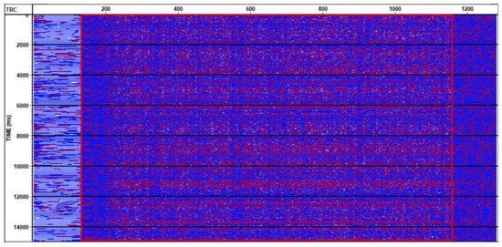
Figure 1.
A fragment of the DAS record before processing. The area of interest highlighted in red is due to the technical peculiarities of the data collection.
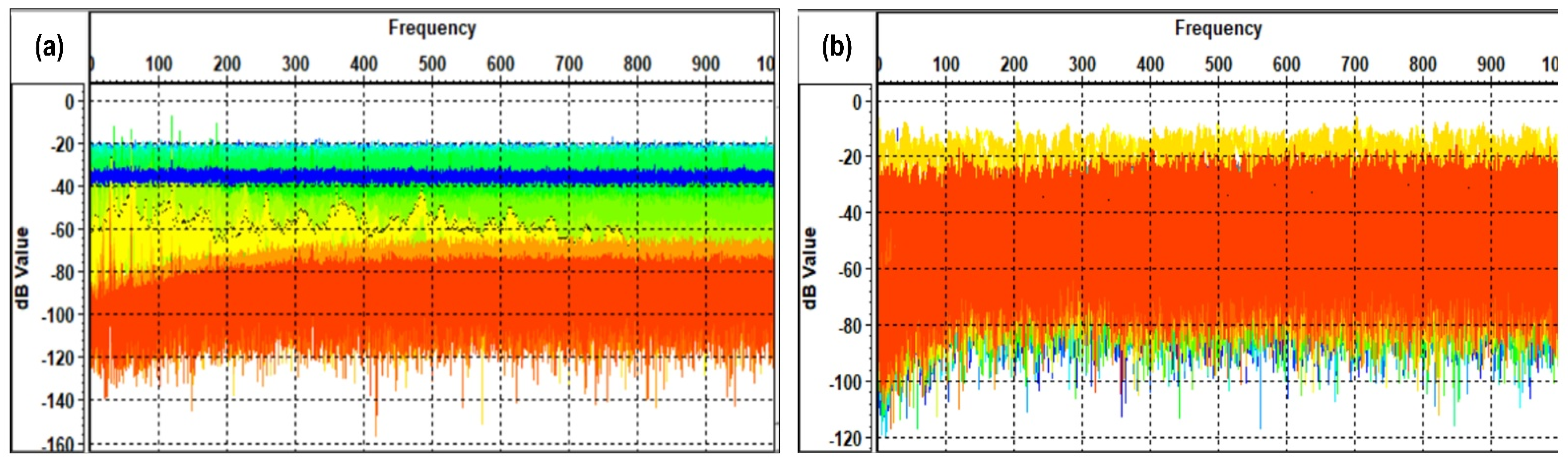
The complete spectral image of the full seismic section in Figure 1 was analyzed before processing the data (Figure 2a). Due to the large variations in signal amplitudes, it is more appropriate to separate the wavefields in the case of DAS data by using a logarithmic scale such as the dB value scale used here.
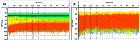
Figure 2.
(a) All traces of the dB spectrum graph display of the DAS data (blue shows the averaged amplitude spectrum over the entire section; the background coherent noise domain is shown in green; orange—the tail part of the record, close to the bottom of the well; the yellow color on the spectrum shows the events we are interested in). (b) The right graph shows the amplitude-frequency spectrum representing the region of interest, depicted in Figure 1 as a red rectangle.
The spectral picture of the full data section can be separated by origin, but after cutting off the entire data area that is not of interest (data outside the red rectangle from the Figure 1), only the spectrum of the target data interval is left (Figure 2b). The spectral image of the area of interest appears to be extremely noise-prone and the separation of the wavefields seems to be a difficult task.
Having established the frequency spectrum of the useful signal, the processing flow in Figure 3 was adopted to achieve the overall goal of improving the SNR. The workflow was based on classical spectral data processing as well as a literature review [57,58,59].

Figure 3.
The DAS data processing workflow.
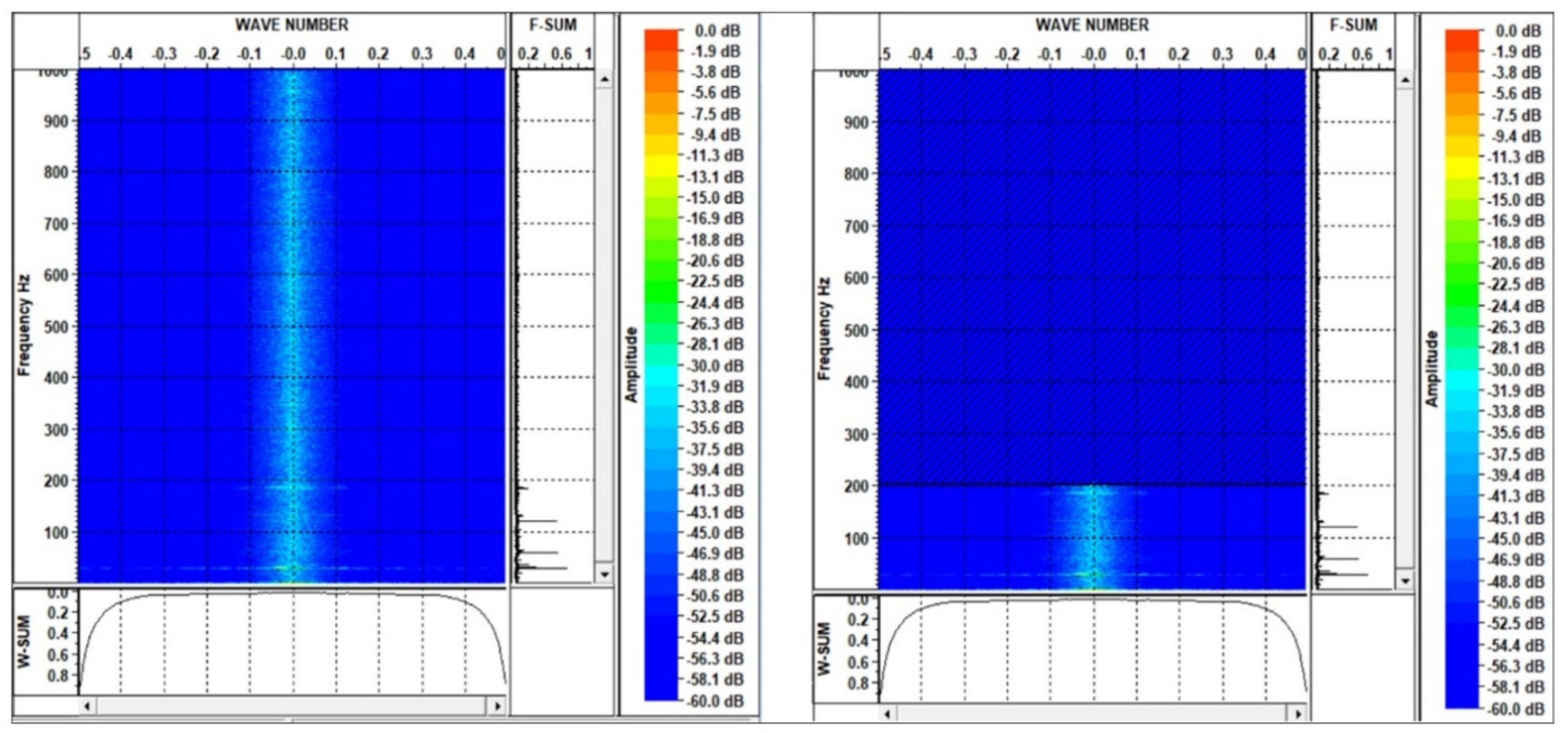
The choice of scaling was due to the high spike values on the seismic profile. The mean scale showed the greatest effectiveness for clarifying the wave pattern. For two-dimensional (2-D) F-k filtering, the horizontal box rejection zone was selected, as shown in Figure 4.

Figure 4.
The original F-k area on the left. The right picture shows the horizontal box rejection zone.
As can be seen in the F-k region beyond 200 Hz, the useful signal is lost and there remains constant noise. In the next step, the remaining noise is filtered out with the band pass Ormsby filter. Analysis of the result at this stage showed the need to apply a 2-D median filter by [58,60] to remove the common mode noise, which appeared as persistent horizontal stripes in the data. As a result of applying the DAS processing graph presented above, we were able to significantly improve the SNR of the data as well as prepare the data for seismic event detection without the loss of useful data (Figure 5).
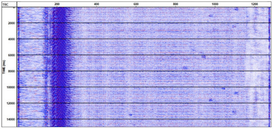
Figure 5.
The results of the DAS data processing using the presented workflow.
2.3. Training Dataset
The training data for the deep neural network was comprised of twenty thousand synthetic microseismic events contaminated with noise from the field data and an equivalent amount of pure noise drawn from the field data, giving a total of forty thousand samples. Each sample comprised of the gathering of receiver responses from 150 receivers used in the forward model. Thus, one sample consisted of 150 seismic traces. A single 1-D anisotropic velocity model with three layers was used in the forward model. The S-wave velocity was taken from the FORGE velocity estimates by Zhang and Pankaw [61] and Wamriew et al. [51], while the P-wave velocities and the densities were estimated using the Castagna [62] and Gardner [63] equations, respectively. Relatively high Thomsen anisotropic parameters [64] of ϵ = 0.51, γ = 0.36, and σ = 0.25, were chosen since previous studies have revealed that a neural network, trained on high anisotropic parameters, would generalize well when presented with waveforms from lower anisotropic models [48]. Table 1 shows the 1-D velocity model used in the study.

Table 1.
The 1-D velocity model used in the forward models.
The monitoring well was set 400 m from the hypothetical treatment well and was arrayed with one hundred and fifty single-component receivers separated at 5 m intervals from a depth of 1050 m downward. This dense spatial sampling was deliberately chosen to match the final downsampled field DAS records. Twenty thousand microseismic events with moment magnitudes between −1.5 and 0.5, similar to the field data, were sampled at random in a two-dimensional plane of a width and depth 700 m × 900 m, respectively. The amplitudes and travel times of the transmitted waves were calculated using ray-tracing. The trapezoidal Ormsby wavelet with low-cut, low-pass, high-cut, and high-pass frequencies was injected at each source point and randomly sampled in the intervals 50–100 Hz, 200–250 Hz, 300–350 Hz, and 400–550 Hz, respectively, to calculate the particle velocity. The data were sampled at a frequency of 2000 Hz for a duration of 1 s. The DAS record is essentially the difference between two geophones over time. Thus, the particle velocity can be converted to the strain-rate using Equation (1) [65]:
where is the dynamic particle velocity at depth location z, and is the converted uniaxial DAS strain-rate in the vertical direction. In this conversion, L is the spatial gauge length. The obtained strain-rates were then amplitude normalized before being added noise from the field data. The noise was spatially downsampled to 5 m, split into a 1 s length by a moving window, and then rescaled to make sure that the amplitudes compared with those of the strain-rates before the addition. Additional 20,000 pure field noise samples were reserved for addition to the training data. A human expert manually inspected the continuous wavelet transform of the noise dataset to ensure that they did not contain any low-magnitude microseismic events. The final step in the preparation of the data involves the conversion of the samples to PNG images of pixel sizes 256 × 256 × 1 ready for use in training the neural network.
2.4. CNN Model Architecture
CNN is a type of deep learning model, which uses a set of kernels to automatically extract the most prominent features from an input dataset. A typical CNN model consists of three layers, namely: convolutional, pooling, and fully connected layers that adaptively learn the outstanding patterns in the input matrix. During the convolution operation, the filter traverses the width and height of the input matrix conducting dot product operation at each data point, resulting in a two-dimensional activation map. The input matrix for the following layer is formed by stacking the activation maps from all filters along the depth dimension of the convolution layer. As a result, the number of filters in the convolution layer matches the depth of the output activation maps. The pooling layer reduces the spatial dimensions of the activation maps and makes them translation invariant to small perturbations by performing a conventional downsampling operation on them. This reduces, to a great deal, the number of future learnable parameters, making CNNs faster to train and capable of handling large volumes of data. The fully connected layer is the decision-making organ of the network. It takes as input the flattened, 1-D activation map outputs from the convolution and pooling layers and maps them into the final outputs of the network.
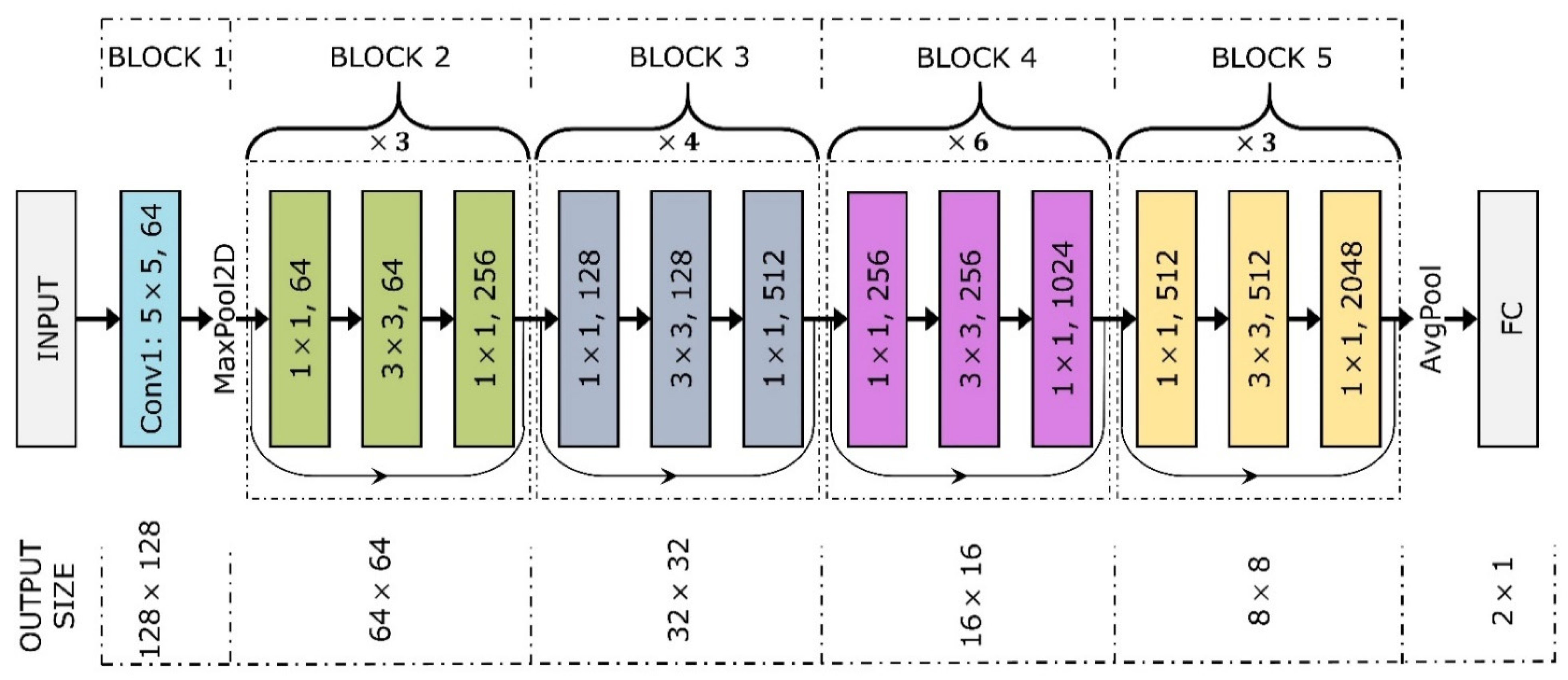
To achieve the objectives of detecting and locating microseismic events from the DAS microseismic data, we designed and employed two deep CNN-based neural networks, namely the residual neural network [66] and an inception-residual neural network [67]. A residual-type deep convolutional neural network [66] comprised of forty-nine convolutional layers, one maxpooling layer, one global average layer, and one fully connected layer. The model was further divided into five blocks with the first block comprised of one convolutional layer with sixty-four filters of dimensions 5 × 5 and stride of 2; a single batch normalization layer; a single 2-D maximum pooling (maxpool2d) layer and a ReLU activation function. The subsequent four blocks were each comprised of equal numbers of convolutional and identity layers. Figure 6 and Table 2 show a detailed representation of the architecture of the neural network model.
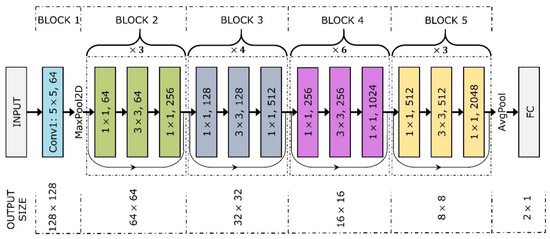
Figure 6.
The architecture of the 50-layer deep neural network used in this study. Abbreviations: Conv—convolutional layer, MaxPool2D—two-dimensional maximum pooling layer, AvgPool—global average pooling layer, FC—fully connected layer.
Table 2.
Details of the 50-layer deep residual neural network used in this study. Abbreviations: Conv—convolution layer, Conv_x—convolution and identity layer.
The network also has residual linkages that help to alleviate the problem of diminishing or exploding gradients by providing an alternative path for the gradient to pass through. The identity layers help to speed up the network training by controlling the number of training parameters. The fifth convolutional block is followed by a 2-D global average pooling layer and the output is then flattened into a 1-D continuous linear vector. A dropout layer is then applied to randomly set 30% of the vector output to zeros in order to avoid overfitting. The result is input into a fully connected layer with a linear activation function and two output nodes to match the expected outputs of the locations of the microseismic events.
The inception-ResNet neural network combines, as the name suggests, the architectures of both the inception and the ResNet models in order to boost its performance. It is comprised of three main building blocks (i.e., the stem block, inception-residual block, and the scaling block). The stem is a pure inception block that forms the input to the neural network. It essentially contains several partitions of sub-networks, which are joined together to form a large network. The partitions provide flexibility for tuning the parameters (e.g., number of filters) of various network layers without affecting the quality of the full network. This block is then followed by an inception-residual block, which uses less expensive inception layers in conjunction with residual layers in order to compensate for the dimension reductions introduced by the inception block. The final block is the scaling block, which scales down the residuals before adding them to the previous layer’s activation. This in turn helps to stabilize the training without the need to manually change the training rate as advocated by He et al. [66]. A detailed description of the inception-ResNet model can be found in [67]. We adopted the inception-resnetv4 model, introducing only changes to the dropout layer (see Section 2.5) and the fully connected. We added a dense layer with two output nodes (for x and z coordinates) with a linear activation function in order to perform the regression. Figure 7 shows the architecture of the network.
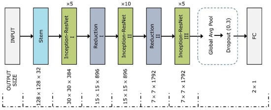
Figure 7.
The architecture of the inception-ResNet. Abbreviations: FC—fully connected layer, Global Avg Pool—global average pooling.
2.5. Neural Network Training and Validation
Before training, a random sample of 1000 events and 1000 noise data together with their corresponding labels were reserved for testing the neural network after training. The remaining 38,000 samples were split as follows: 26,600 for training and 11,400 for validation purposes. The labels were the horizontal (x) and the vertical (z) offsets of the microseismic event sources from the receiver. To solve the regression problem, the noise labels were all initialized with zeros.
The training data were input into the network in batches of sizes of 32. This batch size was arrived at after conducting several trials with a variety of sizes. The tests revealed that while larger batches sped up the training process of the neural network, they significantly reduced the generalization performance of the network. On the other hand, smaller batch sizes considerably increased the training time of the neural network without significant improvements on its convergence. A batch size of 32 was the optimum. While the architecture of our neural network deals effectively with the problem of vanishing gradients by use of the skip connections, it is still susceptible to overfitting due to its complexity. To avoid overfitting, the following measures were taken:
- (i)
- A validation dataset comprising of 30% samples randomly picked from the overall dataset was reserved to assess the performance of the neural network after every epoch of training.
- (ii)
- A dropout layer of 30% was introduced just before the fully-connected layer to set 30% of its input data to zero.
- (iii)
- During training, the performance of the network on the validation dataset was tracked at every epoch and its weights saved only if there was improvement.
- (iv)
- An early-stopping call was introduced to stop the training of the network if there was no improvement in its performance for 20 epochs in a row.
The mean squared error (MSE) loss function was used to train the neural network and its weights updated using the Adam algorithm [68]. Both models were trained on a GeForce GTX 1080 Ti GPU running on 64 cores. The ResNet model trained for 11.8 h and 289 epochs while the inception-ResNet model trained for 7.2 h for 294. Figure 8 shows the metrics training and validation loss and mean absolute errors. The training loss measures the performance of the model on the training dataset while the validation loss measures the performance of the model on the validation dataset.
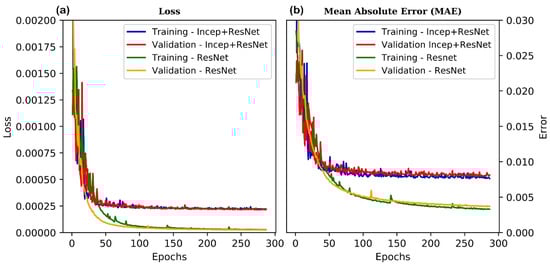
Figure 8.
The training and validation metrics for both the ResNet and inception-ResNet models: (a) training and validation loss; (b) training and validation mean absolute errors.
3. Results
The results of evaluating the trained neural network on the test dataset as well as its application to the field data are reported in this section.
3.1. Evaluation of the Trained Neural Network
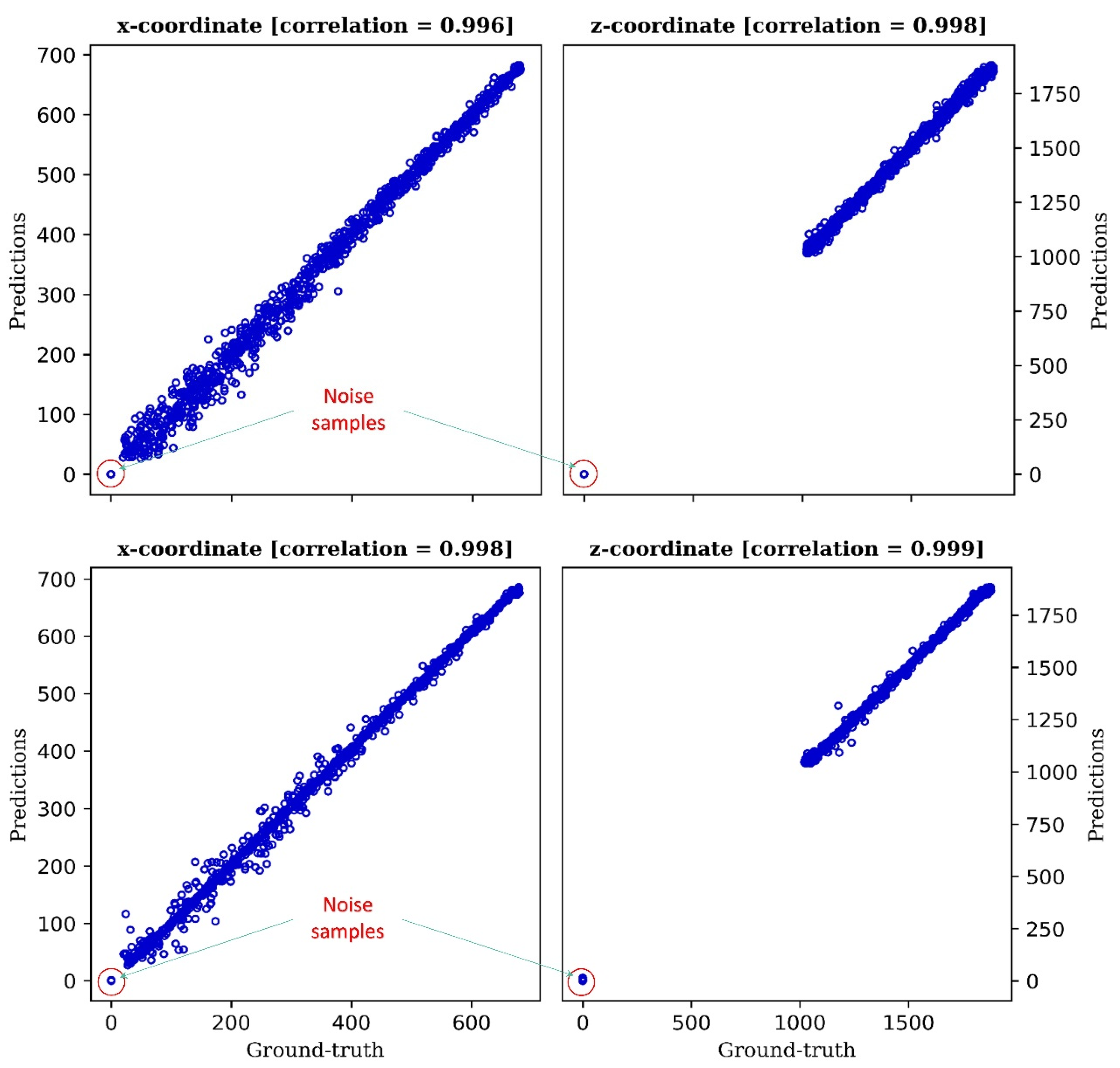
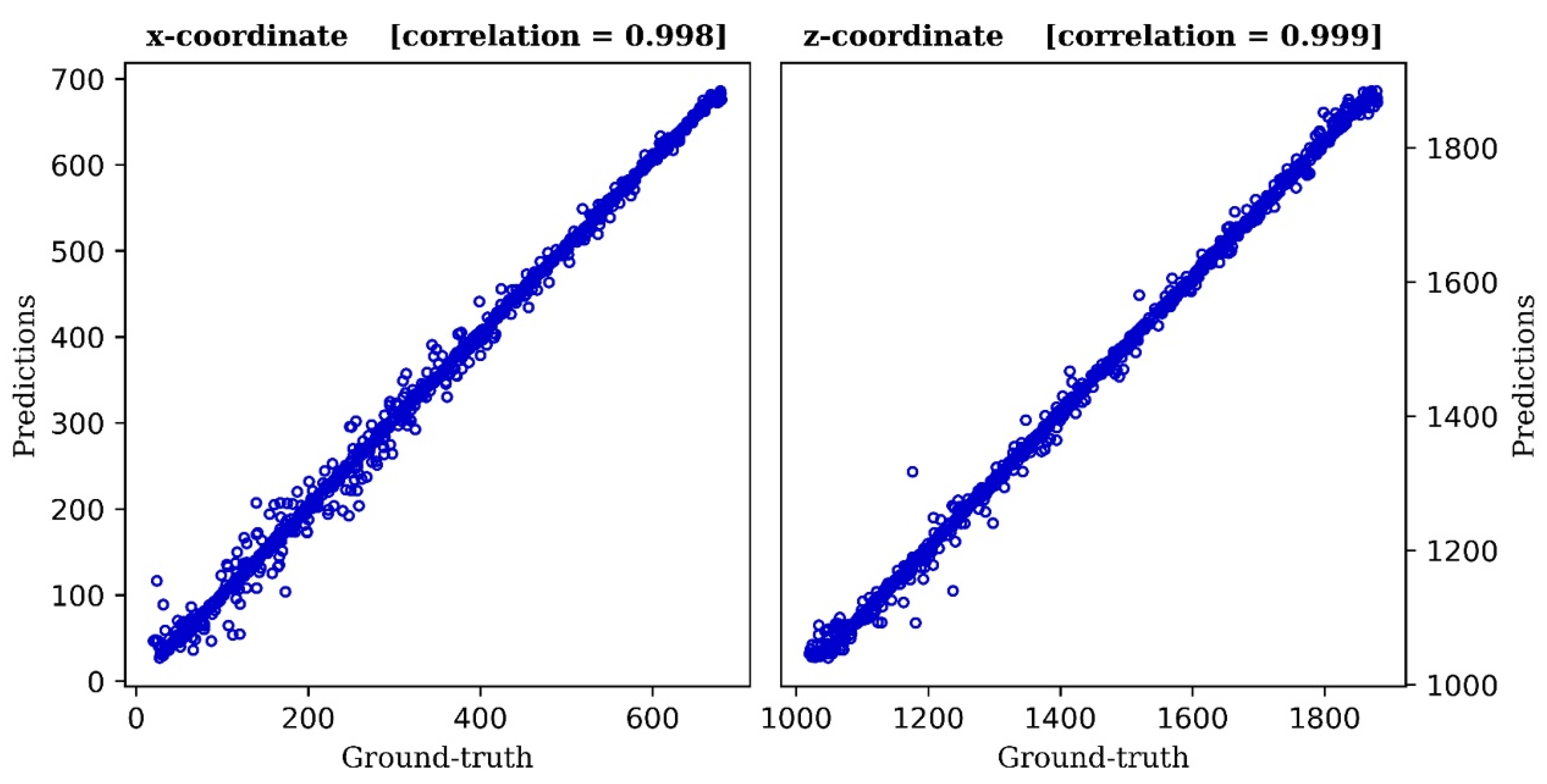
After training the networks, the test dataset comprised of 2000 samples (1000 micro-seismic events and 1000 noise samples) was used to evaluate their performances. Figure 9 shows the correlation plot for the predictions (inverted data) versus the ground-truth (synthetic data) events.
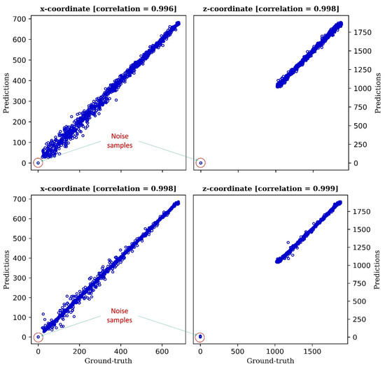
Figure 9.
The correlation plot of the predicted versus ground-truth events. The dots at the origin of both plots are the noise samples. The wide gap in the right plot is because the minimum depth of the microseismic events was 1050 m. Top row: Inception-ResNet output. Bottom row: ResNet output. Pearson correlation coefficient is indicated in the subtitle of each plot. The same correlation plots are shown in Figure 10 after the removal of noise samples from the plots.
As can be seen in both plots, the neural network model correctly distinguished between the noise and microseismic events. The noise was located at the origin (since all noise was labeled with zeros for regression purposes). The Pearson’s product moment correlation coefficient for the predictions and ground-truth values of the x and z coordinates for the inception-ResNet model was 0.996 and 0.998, respectively, while that of the ResNet model was 0.998 and 0.999 for x and z, respectively, as evident in both plots in Figure 9 and Figure 10. This indicates that the predictions are strongly correlated to the ground-truth values and hence are reliable. The ResNet model showed a better correlation than the inception-ResNet model. In Figure 10, we only plotted the output of the ResNet model after the removal of the noise samples.
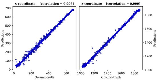
Figure 10.
The correlation plot of the predicted versus ground-truth microseismic events after the exclusion of noise samples from the test dataset.
To measure the trained model’s performance on data that it had not seen before, we performed a statistical analysis of the disparity between the predicted and ground-truth values. Figure 11 shows a plot of the errors versus the ground-truth values for the 1000 microseismic events in the test dataset. The errors here were the differences between the predicted event locations and the ground-truth values. From the plots, it is evident that the errors were centered around zero with a few extreme values, as can be seen in the plots in Figure 11.
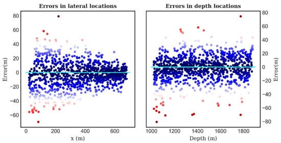
Figure 11.
The errors in the locations of the microseismic events. Dark to medium blue are within two standard deviations from the mean, while red is more than two standard deviations from the mean. The events underlying the cyan line had no errors.
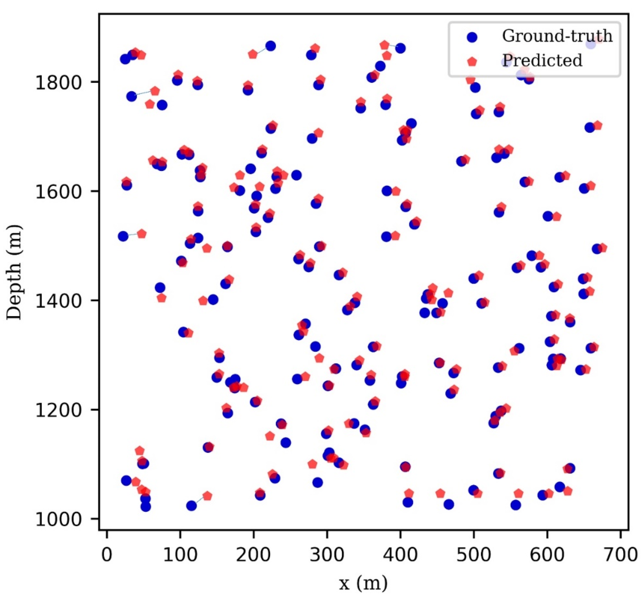
A 2-D section view projection of 150 randomly selected events from the test dataset alongside the inverted (predicted) events is shown in Figure 12. The locations of the predicted events closely matched the benchmark data with minor or no discrepancies in certain cases, as can be seen from the plot. In addition, the distribution of the microseismic events can be seen to spread out in definite patterns, possibly mimicking the fracture network of the reservoir.
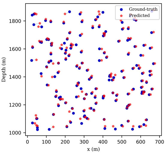
Figure 12.
The 2-D section view project of the predicted versus ground-truth microseismic events. Blue dots represent the ground-truth locations while the red pentagons represent the inverted events.
The calculated statistics for the disparities between the prediction and ground-truth values support the results obtained in Figure 10 and Figure 11, confirming the robustness of the neural network approach. Table 3 presents a summary of the findings. The mean absolute percentages errors (MAPE) in the event locations using the ResNet model were 2.21 and 0.614 for the lateral distance (x) and depth (z) locations, respectively, with the corresponding standard deviations of 11.8 m and 12.0 m.
Table 3.
A summary of the statistical analysis of the uncertainty between the predictions and ground-truth values for the two deep CNNs implemented.
We observed that the mean absolute errors in depth were minimal in both models, but were more spread out, as evident in the standard deviations. This might be attributed to the high values of the anisotropic parameters used in the velocity models as well as the possible uncertainties in the velocity model. Nevertheless, this is necessary for the practical application of the approach, as a good estimate of the velocity model is crucial for the accurate and verifiable inversion of the event locations. Evidently, the ResNet model outperformed the inception-ResNet model by a considerably large margin of errors, as seen in Table 3. However, the inception-ResNet architecture is computationally efficient compared to the ResNet.
3.2. Application to Field Data
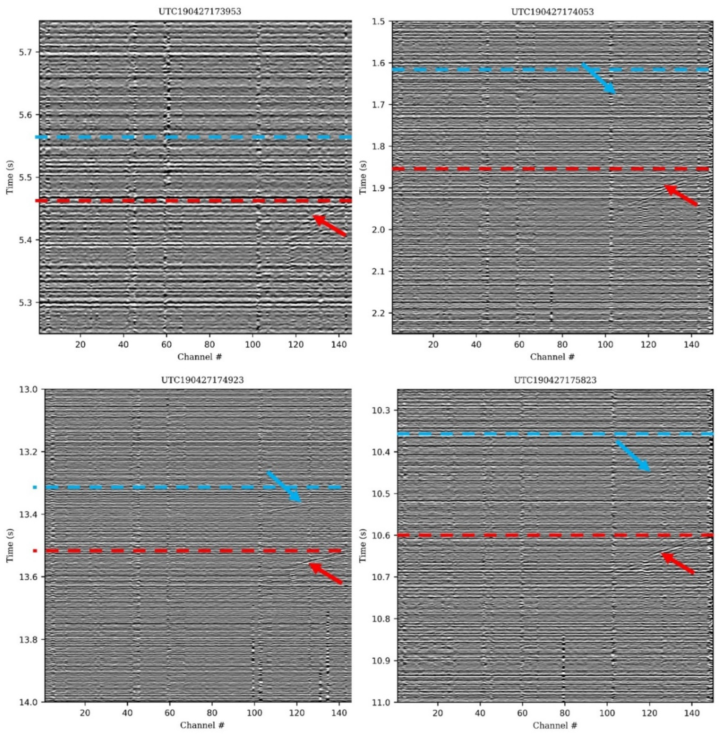
Having evaluated the trained neural network on noise contaminated synthetic data, the neural network was applied to automatically identify and locate microseismic events from the field DAS acquired microseismic data from the FORGE project [55]. This dataset comprises fifteen-second SEG-Y data files of the recording of the hydraulic fracture stimulation experiments conducted in the FORGE reservoir during a period of eleven days. A three-hour subset of this dataset from the seventh and eighth cycles of stages 27 and 28 of the stimulation experiments was chosen for inversion with the deep learning model. This subset has been confirmed to contain thirty microseismic events of varying local magnitudes between −1.5 and 0.5. Each SEG-Y file was split using a one-second length sliding window, giving fifteen samples of 2000 time steps each. The resulting dataset contained 10,800 samples, which were processed as described above in Section 2.1. As a last step, the preprocessed data were amplitude-normalized and converted to greyscale images with pixel sizes of 256 × 256. Then, the data were fed into the pre-trained ResNet neural network for inversion purposes, as it has been proven to be more robust that the inception-ResNet model. The neural network detected and located thirty-six microseismic events. Six of these events were new events, which had not been reported before in the events catalogue. Figure 13 shows a sample of the new events, while Figure 14 shows a 2-D section plot of the inverted event locations.
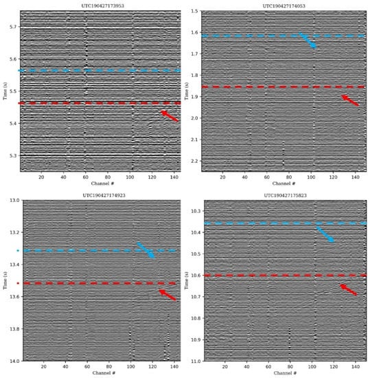
Figure 13.
Sample of the low magnitude events detected by the CNN but were not in the events catalog. The red lines represent the S-wave arrival times while the cyan shows the estimated P-wave arrivals. Similarly, the cyan and red arrows show the P- and S-waves respectively.

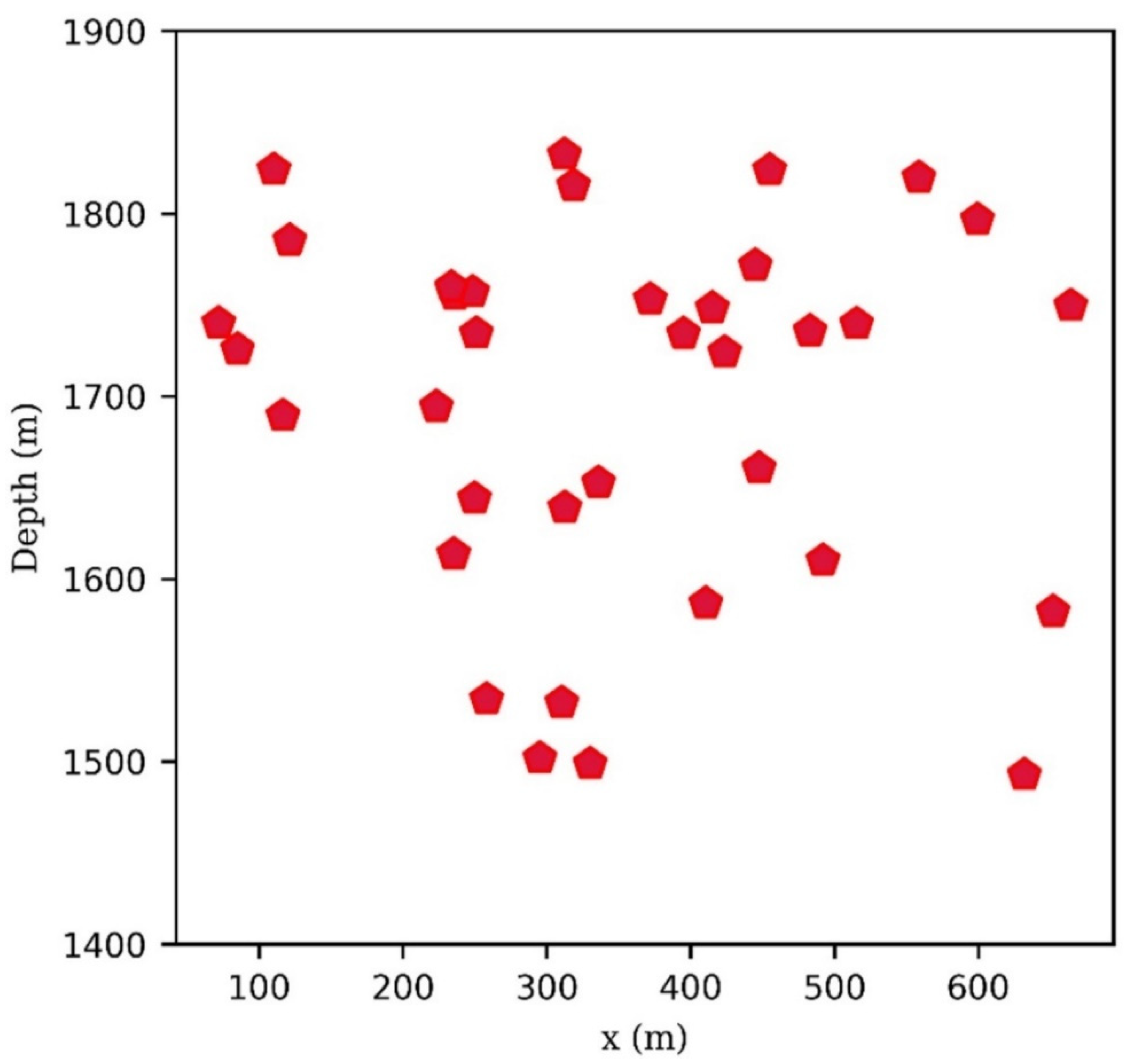
Figure 14.
The 2-D section view projection of the inverted locations of the microseismic events from the FORGE data.
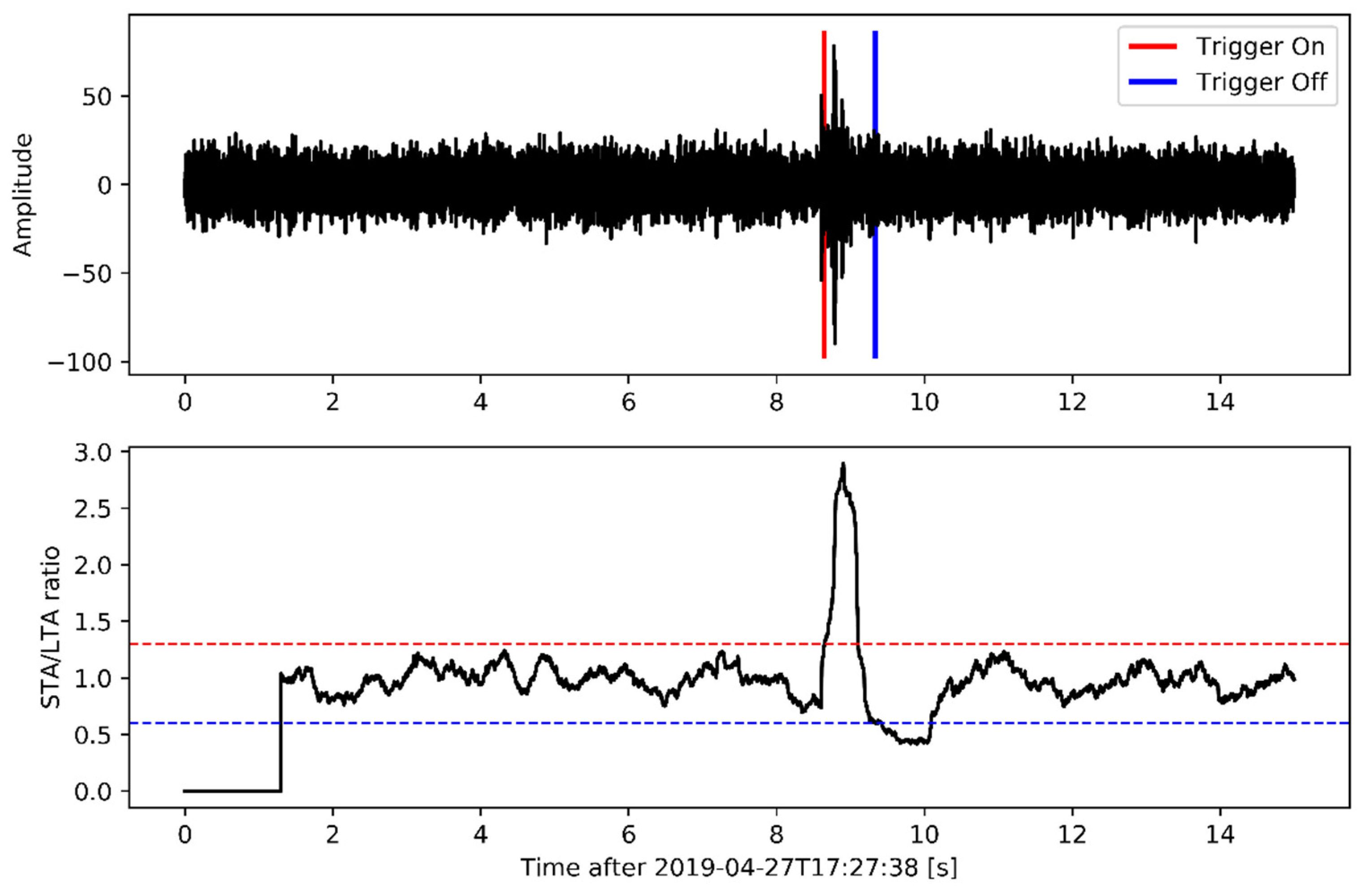
A human expert using the STA/LTA algorithm with STA and LTA windows of lengths of 0.1 s and 1.0 s, respectively, verified the detected events, as shown in Figure 15.
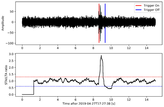
Figure 15.
An example of the STA/LTA implementation for the detection of microseismic events. (Top) Amplitude spectrum of the waveform. (Bottom) STA:LTA ratio plot. An event is declared when the STA:LTA ratio exceeds 1.3. Red and Blue dotted lines indicate the thresholds above and below which the trigger is on and off respectively.
4. Discussion
Microseismic monitoring and analysis has proven to be a valuable screening tool for reservoir characterization, assisting in the calibration and verification of fracture models as well as inferring fracture height, extent, and orientation from wellbore characterization data. In particular, existing fracture properties of a new play as well as the presence of sweet spots in the vicinity of the existing fractures can be well-understood through the analysis of microseismic data. The information gathered during the real-time analysis of microseismic data is vital as it provides knowledge about the progress of each stage of pumping, which is crucial for onsite decision making.
In the preceding sections, we sought to demonstrate the practicality of employing a deep learning approach to invert microseismic data recorded by the fiber optic DAS technology. Deep learning and DAS are both revolutionary technologies with many benefits to the field of microseismic monitoring and analysis. DAS is relatively cheap compared to conventional geophones and accelerometers, is durable, can withstand high downhole pressure, and has a high spatial and temporal resolution, which when fully exploited, provides a detailed mapping of the reservoir. DAS equipment captures massive amounts of data attributable to its high temporal and spatial resolution, making it almost impossible to process and interpret in real-time and poses a challenge for storage space. However, this can be resolved by the use of deep learning. The massive amounts of data that stream in from DAS equipment make it a perfect candidate for deep learning, which leveraging on this advantage, could be applied to train deep neural network models to detect and perform inversions on microseismic data in real-time during reservoir operations. This could expedite the decision-making process for the optimization of the overall goal of the characterization of the reservoir.
The potential of a deep learning approach for detecting and locating microseismic events from DAS records is demonstrated here by results for both synthetic and field records from the hydraulic fracture stimulation project of the FORGE reservoir in Utah, the United States. The CNN model was able to effectively detect and locate thirty-six microseismic events in the DAS data from stages 27 and 28 of the reservoir stimulation, identifying six new weak events that had not been detected previously. The results indicate that the proposed deep learning approach could be applied in real-time during hydraulic fracture stimulation or any other reservoir operations for the simultaneous detection and location of microseismic events or induced seismicity, in the case of passive seismic monitoring.
Integration of the presented method can provide useful information to field engineers that will enable them to make on-the-fly changes to treatment designs, avoid geohazards, locate fault lines that divert fluids and proppants away from the desired fracture zone, and ensure that the spacing between fracture stages is just right. The results of microseismic analysis provide much more information than just the location of individual cracks. The oil and gas industry is learning more about how the reservoir will react to simulated events thanks to the use of microseismic analysis. This allows them to gain a better understanding of how the reservoir will respond to the situation.
In this study, seismic raytracing was used to create the training dataset due to its numerical and computational efficiency and versatility. When conducted in a smoothly changing layered medium, ray tracing can yield dependable approximation solutions with adequate levels of precision. However, because it is simply a rough solution to the elastic wave equation, it can only be used in smooth changing media and may provide inaccurate results in singular regions [69]. For this reason, other robust approaches such as the full waveform inversion and reflectivity methods could be used to generate the training data. In addition, with sufficient computational resources, 3-D velocity models can be used in the forward models, as they can be better constrained than the 1-D models used in this study. The inclusion of well log data could also help to better fine-tune the velocity model and enhance the inversion capability of the neural network in the long run.
Better results could be achieved for the detection of the microseismic events by integrating the proposed approach with well-known conventional algorithms such as template matching and STA/LTA routines, which will enhance the detection threshold of the network, especially in cases when the signal is drowned in noise. For the location of the events, the inclusion of shot/calibration data during training of the network could help to further constrain the network and lower the uncertainties in its prediction. Finally, the integration of 3-C geophone data in addition to DAS could solve the problem of cylindrical symmetry and enable 3-D event location while reducing uncertainty.
5. Conclusions
In this study, a regression-based deep learning approach for detecting and locating microseismic events from seismic waveforms recorded by DAS equipment is presented. Two deep CNN-type neural networks were implemented and their performances compared. The neural network models were trained, validated, and tested on synthetic data injected with noise from the field data. The ResNet outperformed the inception-ResNet model and its feasibility was tested on the field microseismic data from the hydraulic fracture stimulation experiment of the FORGE project. The errors in the location results for the ResNet model were 2.21% and 0.61% for x and z, respectively, while for the inception-ResNet model, they were 3.39% and 0.79% respectively, showing the capability of the proposed deep learning approaches in microseismic data analysis.
The trained neural network can be applied to detect and locate microseismic events in real-time during field operations such as hydraulic fracture stimulation, fluid injection for enhanced oil recovery, and carbon dioxide and hydrogen geosequestration. This will fast-track the field decision making process and in turn optimize the reservoir characterization. A combination of DAS and deep learning for reservoir characterization is revolutionary in the sense that the two approaches complement each other. While DAS records large amounts of data that are almost impossible to process in real-time using conventional routines, deep learning benefits from this since it requires large amounts of data for training and validation. Despite the challenge of single channel recordings, the numerous advantages associated with DAS such as high temporal and spatial resolution, durability, ability to sustain high downhole pressures, and low cost make it a priority choice for microseismic monitoring.
Author Contributions
Conceptualization, D.W., D.B.D., D.B. and R.P.; Data curation, D.W., D.B. and R.P.; Methodology, D.W. and D.B.D.; Resources, D.W., D.B. and E.M.; Software, D.W. and D.B.; Supervision, R.P., M.C., D.P. and D.K.; Validation, D.W., D.B., E.M. and M.C.; Writing—original draft, D.W., D.B.D. and D.B.; Writing—review editing, D.W., D.B.D., D.B., R.P., E.M., M.C., D.P. and D.K. All authors have read and agreed to the published version of the manuscript.
Funding
This work was supported by the Ministry of Science and Higher Education of the Russian Federation under the agreement No. 075-010-2022-011 within the framework of the development program for a World-Class Research Center “Efficient development of the liquid hydrocarbon reserves”.
Data Availability Statement
The field data used in this study are publicly available at http://gdr.openei.org/submissions/1207 (accessed on 5 May 2022). The codes used for the data analysis and to generate the images in this article were written in Python and are partly available here: https://github.com/wamriewdan/DL4Reservoir_Characterization (accessed on 26 June 2022). The data used for training and validating the neural network are confidential. We are happy to release the codes to reproduce all our results on Github on the publication of this paper.
Acknowledgments
The authors would like to express their gratitude to the Energy and Geosciences Institute at the University of Utah for providing the DAS microseismic data from FORGE to the public domain.
Conflicts of Interest
The authors declare no conflict of interest.
References
- IEA. Electricity Market Report, July 2021; Technical Report; IEA: Paris, France, 2021. [Google Scholar] [CrossRef]
- Ozarslan, A. Large-scale hydrogen energy storage in salt caverns. Int. J. Hydrogen Energy 2012, 37, 14265–14277. [Google Scholar] [CrossRef]
- Simon, J.; Ferriz, A.; Correas, L. HyUnder—Hydrogen Underground Storage at Large Scale: Case Study Spain. Energy Procedia 2015, 73, 136–144. [Google Scholar] [CrossRef] [Green Version]
- Osman, A.I.; Mehta, N.; Elgarahy, A.M.; Hefny, M.; Al-Hinai, A.; Al-Muhtaseb, A.H.; Rooney, D.W. Hydrogen production, storage, utilisation and environmental impacts: A review. Environ. Chem. Lett. 2021, 20, 153–188. [Google Scholar] [CrossRef]
- Huang, X.; Meister, L.; Workman, R. Reservoir Characterization by Integration of Time-lapse Seismic and Production Data. In Proceedings of the SPE Annual Technical Conference and Exhibition, San Antonio, TX, USA, 5–8 October 1997; SPE: Houston, TX, USA, 1997. [Google Scholar] [CrossRef]
- Ullo, J. Recent developments in seismic exploration and reservoir characterization. In Proceedings of the 1997 IEEE Ultrasonics Symposium Proceedings. An International Symposium (Cat. No.97CH36118), Toronto, ON, Canada, 5–8 October 1997. [Google Scholar] [CrossRef]
- Jia, A.; Cheng, L. The technique of digital detailed reservoir characterization. Pet. Explor. Dev. 2010, 37, 709–715. [Google Scholar] [CrossRef]
- Eidsvik, J.; Avseth, P.; Omre, H.; Mukerji, T.; Mavko, G. Stochastic reservoir characterization using prestack seismic data. Geophysics 2004, 69, 978–993. [Google Scholar] [CrossRef] [Green Version]
- Aminzadeh, F. Reservoir Characterization: Fundamental and Applications—An Overview; Wiley: Hoboken, NJ, USA, 2021. [Google Scholar] [CrossRef]
- Eisner, L.; Thornton, M.; Griffin, J. Challenges for microseismic monitoring. In SEG Technical Program Expanded Abstracts 2011; Society of Exploration Geophysicists: Houston, TX, USA, 2011. [Google Scholar] [CrossRef] [Green Version]
- García, S.R.M.; Hernández, J.C.; López, J.L.O. Seismic Characterisation using Artificial Intelligence Algorithms for Rock Property Distribution in Static Modeling. In Proceedings of the SPE Reservoir Characterisation and Simulation Conference and Exhibition, Abu Dhabi, United Arab Emirates, 17–19 September 2019; SPE: Houston, TX, USA, 2019. [Google Scholar] [CrossRef]
- Raheem, M.W.; Shuker, A.K. Prediction by reservoir porosity using micro-seismic attribute analysis by machine learning algorithms in an Iraqi Oil Field. Turk. J. Comput. Math. Educ. (TURCOMAT) 2021, 12, 3324–3332. [Google Scholar]
- Afra, S.; Tarrahi, M. An Efficient EOR Screening Approach with Statistical Pattern Recognition: Impact of Rock/Fluid Feature Selection and Extraction. In Proceedings of the Offshore Technology Conference, Houston, TX, USA, 2–5 May 2016. [Google Scholar] [CrossRef]
- Foulger, G.R.; Wilson, M.P.; Gluyas, J.G.; Julian, B.R.; Davies, R.J. Global review of human-induced earthquakes. Earth-Sci. Rev. 2018, 178, 438–514. [Google Scholar] [CrossRef] [Green Version]
- Miller, A.D.; Julian, B.R.; Foulger, G.R. Three-dimensional seismic structure and moment tensors of non-double-couple earthquakes at the Hengill-Grensdalur volcanic complex, Iceland. Geophys. J. Int. 1998, 133, 309–325. [Google Scholar] [CrossRef] [Green Version]
- Keiding, M.; Árnadóttir, T.; Jónsson, S.; Decriem, J.; Hooper, A. Plate boundary deformation and man-made subsidence around geothermal fields on the Reykjanes Peninsula, Iceland. J. Volcanol. Geotherm. Res. 2010, 194, 139–149. [Google Scholar] [CrossRef]
- Pearce, J.K.; Raza, S.S.; Baublys, K.A.; Hayes, P.J.; Firouzi, M.; Rudolph, V. Unconventional CO2 Storage. In Proceedings of the 2021 Asia Pacific Unconventional Resources Technology Conference, Virtual, 16–18 November 2021. [Google Scholar] [CrossRef]
- Williams-Stroud, S.; Bauer, R.; Leetaru, H.; Oye, V.; Stanek, F.; Greenberg, S.; Langet, N. Analysis of Microseismicity and Reactivated Fault Size to Assess the Potential for Felt Events by CO2 Injection in the Illinois Basin. Bull. Seismol. Soc. Am. 2020, 110, 2188–2204. [Google Scholar] [CrossRef]
- Kovacs, T.; Daniel, F.P.; de Dios, C. Strategies for Injection of CO2 into Carbonate Rocks at Hontomin: Final Technical Report; Global CCS Institute, June 2015; Available online: https://www.globalccsinstitute.com/archive/hub/publications/193428/strategies-injection-co2-carbonate-rocks-hontomin-final-technical-report.pdf (accessed on 5 May 2022).
- Simmenes, T.; Hansen, O.R.; Eiken, O.; Teige, G.M.G.; Hermanrud, C.; Johansen, S.; Bolaas, H.M.N.; Hansen, H. Importance of Pressure Management in CO2 Storage. In Proceedings of the Offshore Technology Conference, Houston, TX, USA, 6–9 May 2013. [Google Scholar] [CrossRef]
- Zoback, M.D.; Gorelick, S.M. To prevent earthquake triggering, pressure changes due to CO2 sub-injection need to be limited. Proc. Natl. Acad. Sci. USA 2015, 112, E4510. [Google Scholar] [CrossRef] [Green Version]
- Oye, V.; Aker, E.; Daley, T.M.; Kühn, D.; Bohloli, B.; Korneev, V. Microseismic Monitoring and Interpretation of Injection Data from the in Salah CO2 Storage Site (Krechba), Algeria. Energy Procedia 2013, 37, 4191–4198. [Google Scholar] [CrossRef] [Green Version]
- Abe, J.; Popoola, A.; Ajenifuja, E.; Popoola, O. Hydrogen energy, economy and storage: Review and recommendation. Int. J. Hydrogen Energy 2019, 44, 15072–15086. [Google Scholar] [CrossRef]
- Tarkowski, R. Underground hydrogen storage: Characteristics and prospects. Renew. Sustain. Energy Rev. 2019, 105, 86–94. [Google Scholar] [CrossRef]
- Lemieux, A.; Shkarupin, A.; Sharp, K. Geologic feasibility of underground hydrogen storage in Canada. Int. J. Hydrogen Energy 2020, 45, 32243–32259. [Google Scholar] [CrossRef]
- Heinemann, N.; Wilkinson, M.; Haszeldine, R.S.; Fallick, A.E.; Pickup, G.E. CO2 sequestration in a UK North Sea analogue for geological carbon storage. Geology 2013, 41, 411–414. [Google Scholar] [CrossRef]
- Simpson, D.W.; Leith, W. The 1976 and 1984 Gazli, USSR, earthquakes—Were they induced? Bull. Seismol. Soc. Am. 1985, 75, 1465–1468. [Google Scholar]
- Maxwell, S.C.; Urbancic, T.I. The role of passive microseismic monitoring in the instrumented oil field. Lead. Edge 2001, 20, 636–639. [Google Scholar] [CrossRef] [Green Version]
- Ajayi, B.; Walker, K.; Sink, J.; Wutherich, K.; Downie, R. Using Microseismic Monitoring as a Real Time Completions Diagnostic Tool in Unconventional Reservoirs: Field Case Studies. In Proceedings of the SPE Eastern Regional Meeting, Columbus, OH, USA, 17–19 August 2011; SPE: Houston, TX, USA, 2011. [Google Scholar] [CrossRef]
- Mateeva, A.; Lopez, J.; Potters, H.; Mestayer, J.; Cox, B.; Kiyashchenko, D.; Wills, P.; Grandi, S.; Hornman, K.; Kuvshinov, B.; et al. Distributed acoustic sensing for reservoir monitoring with vertical seismic profiling. Geophys. Prospect. 2014, 62, 679–692. [Google Scholar] [CrossRef]
- Mestayer, J.; Cox, B.; Wills, P.; Kiyashchenko, D.; Lopez, J.; Costello, M.; Bourne, S.; Ugueto, G.; Lupton, R.; Solano, G.; et al. Field trials of distributed acoustic sensing for geophysical monitoring. In SEG Technical Program Expanded Abstracts 2011; Society of Exploration Geophysicists: Houston, TX, USA, 2011. [Google Scholar] [CrossRef]
- Walter, F.; Gräff, D.; Lindner, F.; Paitz, P.; Köpfli, M.; Chmiel, M.; Fichtner, A. Distributed acoustic sensing of microseismic sources and wave propagation in glaciated terrain. Nat. Commun. 2020, 11, 2436. [Google Scholar] [CrossRef]
- Hudson, T.S.; Baird, A.F.; Kendall, J.M.; Kufner, S.K.; Brisbourne, A.M.; Smith, A.M.; Butcher, A.; Chalari, A.; Clarke, A. Distributed Acoustic Sensing (DAS) for Natural Microseismicity Studies: A Case Study From Antarctica. J. Geophys. Res. Solid Earth 2021, 126, e2020JB021493. [Google Scholar] [CrossRef]
- Lellouch, A.; Luo, B.; Huot, F.; Clapp, R.G.; Given, P.; Biondi, E.; Nemeth, T.; Nihei, K.T.; Biondi, B.L. Microseismic analysis over a single horizontal distributed acoustic sensing fiber using guided waves. Geophysics 2022, 87, KS83–KS95. [Google Scholar] [CrossRef]
- Liu, Y.; Wu, K.; Jin, G.; Moridis, G.; Kerr, E.; Scofield, R.; Johnson, A. Fracture-Hit Detection Using LF-DAS Signals Measured during Multifracture Propagation in Unconventional Reservoirs. SPE Reserv. Eval. Amp Eng. 2020, 24, 523–535. [Google Scholar] [CrossRef]
- Ichikawa, M.; Kato, M.; Uchida, S.; Tamura, K.; Kato, A.; Ito, Y.; Groot, M. Low Frequency Das Data Study with Integrated Data Analysis for Monitoring Hydraulic Fracture. In Proceedings of the 82nd EAGE Annual Conference & Exhibition, Amsterdam, The Netherlands, 18–21 October 2021; European Association of Geoscientists & Engineers: Bunnik, The Netherlands, 2021. [Google Scholar] [CrossRef]
- Van der Horst, J.; den Boer, H.; in’t Panhuis, P.; Kusters, R.; Roy, D.; Ridge, A.; Godfrey, A. Fibre Optic Sensing for Improved Wellbore Surveillance. In Proceedings of the International Petroleum Technology Conference, Beijing, China, 26–28 March 2013. [Google Scholar] [CrossRef]
- Finfer, D.C.; Mahue, V.; Shatalin, S.V.; Parker, T.R.; Farhadiroushan, M. Borehole Flow Monitoring using a Non-intrusive Passive Distributed Acoustic Sensing (DAS). In Proceedings of the SPE Annual Technical Conference and Exhibition, Amsterdam, The Netherlands, 27–29 October 2014; SPE: Houston, TX, USA, 2014. [Google Scholar] [CrossRef]
- Naldrett, G.; Cerrahoglu, C.; Mahue, V. Production Monitoring Using Next-Generation Distributed Sensing Systems. Petrophys.—SPWLA J. Form. Eval. Reserv. Descr. 2018, 59, 496–510. [Google Scholar] [CrossRef]
- LeCun, Y.; Bengio, Y.; Hinton, G. Deep learning. Nature 2015, 521, 436–444. [Google Scholar] [CrossRef]
- Binder, G.; Tura, A. Convolutional neural networks for automated microseismic detection in downhole distributed acoustic sensing data and comparison to a surface geophone array. Geophys. Prospect. 2020, 68, 2770–2782. [Google Scholar] [CrossRef]
- Huot, F.; Lellouch, A.; Given, P.; Luo, B.; Clapp, R.G.; Nemeth, T.; Nihei, K.T.; Biondi, B.L. Detection and characterization of microseismic events from fiber-optic DAS data using deep learning. arXiv 2022, arXiv:2203.07217. [Google Scholar]
- Qu, S.; Guan, Z.; Verschuur, E.; Chen, Y. Automatic high-resolution microseismic event detection via supervised machine learning. Geophys. J. Int. 2020, 222, 1881–1895. [Google Scholar] [CrossRef]
- Hernandez, P.D.; Ramirez, J.A.; Soto, M.A. Deep-Learning-Based Earthquake Detection for Fiber-Optic Distributed Acoustic Sensing. J. Lightwave Technol. 2022, 40, 2639–2650. [Google Scholar] [CrossRef]
- Shaheen, A.; bin Waheed, U.; Fehler, M.; Sokol, L.; Hanafy, S. GroningenNet: Deep Learning for Low-Magnitude Earthquake Detection on a Multi-Level Sensor Network. Sensors 2021, 21, 8080. [Google Scholar] [CrossRef]
- Mousavi, S.M.; Ellsworth, W.L.; Zhu, W.; Chuang, L.Y.; Beroza, G.C. Earthquake transformer—An attentive deep-learning model for simultaneous earthquake detection and phase picking. Nat. Commun. 2020, 11, 3952. [Google Scholar] [CrossRef] [PubMed]
- Kuyuk, H.S.; Susumu, O. Real-Time Classification of Earthquake using Deep Learning. Procedia Comput. Sci. 2018, 140, 298–305. [Google Scholar] [CrossRef]
- Wamriew, D.; Charara, M.; Pissarenko, D. Joint event location and velocity model update in real-time for downhole microseismic monitoring: A deep learning approach. Comput. Geosci. 2022, 158, 104965. [Google Scholar] [CrossRef]
- Tanaka, R.; Naoi, M.; Chen, Y.; Yamamoto, K.; Imakita, K.; Tsutsumi, N.; Shimoda, A.; Hiramatsu, D.; Kawakata, H.; Ishida, T.; et al. Preparatory acoustic emission activity of hydraulic fracture in granite with various viscous fluids revealed by deep learning technique. Geophys. J. Int. 2021, 226, 493–510. [Google Scholar] [CrossRef]
- Huot, F.; Biondi, B. Machine learning algorithms for automated seismic ambient noise processing applied to DAS acquisition. In SEG Technical Program Expanded Abstracts 2018; Society of Exploration Geophysicists: Houston, TX, USA, 2018. [Google Scholar] [CrossRef]
- Wamriew, D.; Pevzner, R.; Maltsev, E.; Pissarenko, D. Deep Neural Networks for Detection and Location of Microseismic Events and Velocity Model Inversion from Microseismic Data Acquired by Distributed Acoustic Sensing Array. Sensors 2021, 21, 6627. [Google Scholar] [CrossRef]
- Huot, F.; Biondi, B.L.; Clapp, R.G. Detecting local earthquakes via fiber-optic cables in telecommunication conduits under Stanford University campus using deep learning. arXiv 2022, arXiv:2203.05932. [Google Scholar]
- Martin, T.; Nash, G. Utah FORGE: High-Resolution DAS Microseismic Data from Well 78-32; Technical Report; USDOE Geothermal Data Repository (United States); Energy and Geoscience Institute at the University of Utah: Salt Lake City, UT, USA, 2019. [Google Scholar]
- Moore, J.; Simmons, S.; McLennan, J.; Jones, C.; Skowron, G.; Wannamaker, P.; Nash, G.; Hardwick, C.; Hurlbut, W.; Allis, R.; et al. Utah FORGE: Phase 2C Topical Report; Technical Report; DOE Geothermal Data Repository; Energy and Geoscience Institute at the university of Utah: Salt Lake City, UT, USA, 2019. [Google Scholar]
- Taylor, M.; Greg, N. Utah FORGE: High-Resolution DAS Microseismic Data from Well 78-32 [Data Set]. Open EI GDR 2019. [Google Scholar]
- Dok, R.V.; Fuller, B.; Bianco, R. Design, acquisition, and processing of three Permian Basin 3D VSP surveys to support the processing and interpretation of a large 3D/3C surface seismic survey. In Proceedings of the First International Meeting for Applied Geoscience & Energy Expanded Abstracts, Denver, CO, USA, 26 September–1 October 2021; Society of Exploration Geophysicists: Houston, TX, USA, 2021. [Google Scholar] [CrossRef]
- Lellouch, A.; Biondi, B.L. Seismic Applications of Downhole DAS. Sensors 2021, 21, 2897. [Google Scholar] [CrossRef]
- Duncan, G.; Beresford, G. Median filter behaviour with seismic data1. Geophys. Prospect. 1995, 43, 329–345. [Google Scholar] [CrossRef]
- Ipatov, A.I.; Andrianovsky, A.V.; Gubarev, A.Y.; Voronkevich, A.V.; Galimzyanov, R.M.; Solovyova, V.V. Study of seismoacoustic effects in a producing oil horizontal well based on a fiber-optic cable sensor DAS. PROneft’ Proffessional’no O Nefti. 2021, 6, 50–57. [Google Scholar] [CrossRef]
- Justusson, B.I. Median Filtering: Statistical Properties. In Two-Dimensional Digital Signal Processing II: Transform and Median Filters; Topics in Applied Physics; Springer: Berlin/Heidelberg, Germany, 1981; pp. 161–196. [Google Scholar] [CrossRef]
- Zhang, H.; Pankow, K.L. High-resolution Bayesian spatial autocorrelation (SPAC) quasi-3-D model of Utah FORGE site with a dense geophone array. Geophys. J. Int. 2021, 225, 1605–1615. [Google Scholar] [CrossRef]
- Castagna, J.P.; Batzle, M.L.; Eastwood, R.L. Relationships between compressional-wave and shear-wave velocities in clastic silicate rocks. Geophysics 1985, 50, 571–581. [Google Scholar] [CrossRef]
- Gardner, G.H.F.; Gardner, L.W.; Gregory, A.R. Formation velocity and density—The diagnostic basics for stratigraphic traps. Geophysics 1974, 39, 770–780. [Google Scholar] [CrossRef] [Green Version]
- Thomsen, L. Weak elastic anisotropy. Geophysics 1986, 51, 1954–1966. [Google Scholar] [CrossRef]
- Bakku, S.K. Fracture Characterization from Seismic Measurements in a Borehole. Ph.D. Thesis, Massachusetts Institute of Technology, Cambridge, MA, USA, 2015. [Google Scholar]
- He, K.; Zhang, X.; Ren, S.; Sun, J. Deep Residual Learning for Image Recognition. arXiv 2015, arXiv:1512.03385. [Google Scholar]
- Szegedy, C.; Ioffe, S.; Vanhoucke, V.; Alemi, A. Inception-v4, Inception-ResNet and the Impact of Residual Connections on Learning. arXiv 2016, arXiv:1602.07261. [Google Scholar]
- Kingma, D.P.; Ba, J. Adam: A Method for Stochastic Optimization. arXiv 2014, arXiv:1412.6980. [Google Scholar]
- Červený, V.; Pšenčík, I. Seismic, Ray Theory. In Encyclopedia of Solid Earth Geophysics; Springer: Amsterdan, The Netherlands, 2011; pp. 1244–1258. [Google Scholar] [CrossRef]


Publisher’s Note: MDPI stays neutral with regard to jurisdictional claims in published maps and institutional affiliations. |
© 2022 by the authors. Licensee MDPI, Basel, Switzerland. This article is an open access article distributed under the terms and conditions of the Creative Commons Attribution (CC BY) license (https://creativecommons.org/licenses/by/4.0/).