Abstract
Remote sensing technology allows to provide information about biochemical and biophysical crop traits and monitor their spatiotemporal dynamics of agriculture ecosystems. Among multiple retrieval techniques, hybrid approaches have been found to provide outstanding accuracy, for instance, for the inference of leaf area index (LAI), fractional vegetation cover (fCover), and leaf and canopy chlorophyll content (LCC and CCC). The combination of radiative transfer models (RTMs) and data-driven models creates an advantage in the use of hybrid methods. Through this review paper, we aim to provide state-of-the-art hybrid retrieval schemes and theoretical frameworks. To achieve this, we reviewed and systematically analyzed publications over the past 22 years. We identified two hybrid-based parametric and hybrid-based nonparametric regression models and evaluated their performance for each variable of interest. From the results of our extensive literature survey, most research directions are now moving towards combining RTM and machine learning (ML) methods in a symbiotic manner. In particular, the development of ML will open up new ways to integrate innovative approaches such as integrating shallow or deep neural networks with RTM using remote sensing data to reduce errors in crop trait estimations and improve control of crop growth conditions in very large areas serving precision agriculture applications.
1. Introduction
The importance of robust retrieval of crop traits in the agricultural sector has been endorsed by the Global Climate Observing System and reported in IPCC Sixth Evaluation [1]. Demand for food will increase in the future in order to feed a constantly growing human population. Currently, the total global population is around 7.86 billion and the Food and Agriculture Organization of the United Nations (FAO) estimates that it will increase to 11.2 billion by the end of the 21st century. To meet estimated world nutrition needs, it is necessary to boost crop production. However, climatic change is likely to cause a reduction in crop productivity in terms of quality and quantity, resulting in a progressive burden on the ecosystem [2]. Thus, intervention in agriculture is necessary in order to obtain not only high quantity yields but also high-quality yields while remaining economically perspective [3].
To maintain crop productivity, croplands should be monitored during the growth cycle, noting the changes in crop status that are manifested in biophysical (e.g., leaf area index (LAI), fractional vegetation cover (fCover)) and biochemical (e.g., chlorophyll content (CC) at leaf (LCC) and canopy (CCC) levels) variables. Where an abatement in yield can be anticipated, for example, due to climate change, feasible measures must be undertaken to avoid nutrient deficiencies in the population [4]. A precise management approach needs to be adopted by providing accurate supplies of fertilizers (organic or non-organic), pesticides, and irrigation taking into account inter- and intra-field variability in crops [5]. This method is known as precision agriculture (PA), and endeavors to reduce and optimize the cost of inputs by using multiple sources of data informing about spatial and temporal variability of the crops and soil sites [6].
For providing such data in a continuous and non-destructive way, remote sensing (RS) technology provides an affordable and environmentally friendly tool to assess crop area, type, and condition (e.g., diseases, plant pests, and plant stress states) in near-real time along the season [7]. In this context, the continuous growth of space-based platforms, such as airborne, unmanned aerial vehicles (UAV), and satellite remote sensing, along with in situ observation, creates the potential to offer reliable and repeatable coverage of Earth observation datasets. These will support and help farmers as well as national and international ministries of agriculture for management and decision-making. In optical RS, the visible near-infrared spectrum (VNIR) and short-wave infrared (SWIR) are often used to record information about the state and dynamics of vegetation. This information is acquired by the sensors that are implemented, making it possible for multispectral and hyperspectral imaging [8]. Each of these images has different spatial, spectral, and temporal resolutions. Multispectral imagery (e.g., Landsat, Sentinel 2, and SPOT) contains a limited number of spectral bands. On the other hand, hyperspectral images (e.g., PROBA-1, HyspIRI, Hyperion, and CASI) provide multiple bands that help detect subtle variations of ground covers and their changes over time [9]. Therefore, the performance of hyperspectral data is outperformed in monitoring crop traits and has attracted researchers, e.g., estimating LAI [10], fCover [11,12,13], and CC [14,15].
Since the advent of RS science, a diversity of retrieval methods has been employed to link spectral reflectance with biophysical and biochemical traits. The earliest approaches were (i) variable data-driven, i.e., empirical statistical approaches from a practical experiment in 1970, and (ii) radiometric data-driven, also referred to as physically-based approaches or radiative transfer modeling (RTM), appearing in the 1980s [16,17]. During the last two decades, hybrid retrieval approaches have paved the road to make the use of both fundamental approaches (variable and radiometric data-driven) in a synergistic way. Verrelst et al. [18] and Verrelst et al. [19] updated the actual taxonomy of the retrieval methods into four main groups: (1) parametric regression methods follow an empirical statistical approach, which postulates the explicit relationship between the spectra bands as predictors and the interested canopy variable as the dependent variable. (2) Nonparametric regression methods are preferred for use due to fewer limitations in using the number of spectrum bands and in the type of data distribution as compared to the previous method [20]. The non-explicit relationship between the feature spectrum and the target parameters is assumed, which means that the relationship forum is not predetermined. This method is divided into two classes: linear and nonlinear regression models. (3) Physically-based canopy trait retrieval method is grounded by radiative transfer theory, which is a mathematical model that describes the interaction between solar radiation and vegetation canopies. Over the past four decades, a diversity of vegetation radiative transfer models (RTM) have been developed, simulating the optical properties and radiative interactions of leaves, canopies, and soil (e.g., see [21] for a comparison). (4) Hybrid methods are the combination of physically-based canopy trait retrieval methods with data-driven models (parametric and nonparametric).
A retrieval approach is used to model Earth observation (EO) data. With the advancement of remote sensing tools, the acquisition of EO data has increased the data archive beyond dozens of 65 petabytes [22]. It increases the dimensions of the data structure in terms of spatial, spectral, and temporal resolution. Thus, these big data require computational power to analyze, process, and create large-scale crop mapping [23,24]. The developed method of hybrid retrieval has the ability to speed up the processing chain and find complex relationships between the canopy reflectance and the variable of interest to obtain useful information about crop traits [22]. In addition, thanks to the synergistic use of both mechanical (RTM) and data-driven methods (either parametric or nonparametric), the ground in situ data are not urgently required in the simulation process but can mainly be used for validation. Different studies have proved the efficiency of using such a method in terms of the accuracy of estimates and mapping crop variables at local and global scales [25,26,27,28,29,30,31].
Indeed, the terminology of a hybrid approach is widely denominated when combining at least two methods, as claimed in the study of [32]. For instance, the hybrid method can be a combination of a crop growth model (CGM) with a canopy RTM [33,34], a geometric and a turbid medium model to represent the canopy in three-dimensional (3D) space RTM [35], a geostatistical method with machine learning (ML) [36], or blending two methods of MLs [37]. Verrelst et al. [18] and Berger et al. [32] exemplified the conceptual framework of retrieval strategies, including the hybrid method based on a combination of RTMs with MLs for estimating vegetation traits. However, some studies used vegetation indices instead of ML to retrieve the targeted variable(s) based on the simulated spectra of the RTM [38,39]. Hence, there is no consensus about the exact terminology of a hybrid retrieval method, i.e., the types of methods that may contribute to quantifying the vegetation properties of interest.
Therefore, there is still a need to clarify the conceptual framework for the hybrid retrieval methods, including a description of the basic idea of both approaches, parametric and nonparametric, based on radiative transfer model simulation. To date, no review paper has been devoted to depicting this optical retrieval method in a detailed manner, although a variety of retrieval approaches (such as RTM and empirical statistical model using them as an independent unit) are available to determine the essential vegetation characteristics in the agriculture application. The review paper aims to provide a comprehensive overview of the application of hybrid retrieval methods in the field of quantitative RS, exemplarily, for retrieving LAI, fCover, and CC. Our paper is structured into several main aspects as follows: In Section 2, the state-of-the-art hybrid approaches are explained by providing the conceptual framework. Section 3 describes techniques that handle the simulated spectra obtained from the radiative transfer model. The scientific literature over the past two decades (from 2000 to 2022) was analyzed, as illustrated in Section 4. Section 5 and Section 6 are devoted to presenting the results in the form of bar and pie charts and drawing the conclusion and future perspective.
2. The Conceptual Frameworks of Hybrid Retrieval Methods
The foundation of optical remote sensing is radiative transfer models (RTMs), which describe the interaction of matter and electromagnetic radiation [40]. RTM (deterministic models) is an effective tool for precise retrievals of Earth attributes from satellite data and is used in a variety of contexts, including the calibration of radiometric sensors, atmospheric correction, and the modeling radiation processes in vegetation canopies [22]. In canopy radiative transfer models, the link between leaf and canopy parameters and reflectance, absorbance, and scattering mechanisms has been investigated [40,41,42,43]. According to the complex structure of plants, various types of canopy RTMs have been proposed, starting from the simple turbid medium model (1D) to the advanced Monte Carlo model, which allows a clear representation of complex 3D canopy structures [21,44,45,46]. The most established method of canopy modeling is to calculate the reflectance from the top of the canopy (TOC) by coupling the leaf optical properties model and the canopy reflectance model to the soil reflectance model (e.g., PROSAIL [47]). This aids to investigate how other disturbing elements, such as soil background, nonphotosynthetic materials, and observation geometry, affect canopy reflectance [48]. When combining the canopy reflectance models with the atmosphere, the radiance from the top of the atmosphere (TOA), which is detected by the sensor, can be computed [41,49]. To estimate leaf traits and canopy properties either from TOC reflectance or TOA radiance data, the retrieval method as the core of a retrieval system is needed [16].
The hybrid retrieval method, as the main focus of this research, is to link both models of canopy radiative transfer with the data-driven model. Analytically, a hybrid retrieval workflow consists of two parts: first, establishing the lookup table (LUT database) for simulating canopy spectra based on the predefined input parameters of RTM, and second, applying a data-driven model (statistical methods) to simulations to estimate crop traits. These simulations are determined according to spectral configuration for the particular sensor. To search for the optimal simulated spectra closed to the measured spectra, two methods are available to use, either the parametric or nonparametric regression method. Selecting either of them depends on the types of sensors in remote sensing used. Many studies prefer to use a nonparametric method with hyperspectral data due to its ability to handle the high dimensions of the spectra and resistance against noise and spectrum uncertainty [50]. This method is distinguished by its outstanding predictive power and can be efficiently applied over the entire satellite images at a global or local scale to map the functional traits of plants. This is not the case for the parametric method when using multispectral data. Any of the retrieval methods, whether parametric or nonparametric, can apply to these data, and this depends on the objective of the study.
The benefit of hybrid retrieval methods is that they mimic a wide range of land cover scenarios (up to hundreds of thousands), resulting in a data collection far larger than what can be obtained during a field study [20]. Hence, a large amount of in situ data is not required; only a few samples are needed to validate the estimations. Keep in mind that the developed retrieval method does not mitigate the nature of the ill-posed problem, which often renders unstable results and uncertainties of results. To alleviate this problem, prior information related to the correlation and distribution of the canopy variables [51,52] and/or use additional information of spatial, temporal [53,54,55], both of them, or multi-angular observation data [56] were integrated with LUT approach in the RTM. Figure 1 shows an overview of the hybrid retrieval methodology, including regression models. They are described in the following Section 2.1 and Section 2.2.

Figure 1.
General workflow for the hybrid retrieval methodology.
2.1. Hybrid Modeling Based on Parametric Regression Methods
Over the last two decades, parametric models based on physical models have been pronounced in the science of vegetation analysis to obtain universal indices applicable under different environmental conditions. Given the various scenarios of synthetic canopy spectra and their corresponding canopy characteristics, a hybrid model can be utilized to create a new index or optimize and evaluate the robustness of vegetation indices (VIs), shape indices, and spectral transformation techniques. In general, these techniques create a regression model in which a few spectral bands with high sensitivity are selected for the variable of interest. In the hybrid retrieval method, the generated regression model is applied to simulation and experimental data. Then, the cost function is used to reduce the discrepancy between the observed indicator and the simulation. To select the best VIs for predicting canopy characteristics, the curve-fitting models are used to construct the relationship between the targeted variable and index. These models can be linear, exponential, power, logarithmic, or polynomial regression. Finally, the implementation of a validation procedure using empirical measurements is a necessary and final step to verify the accuracy of the estimation of the variable of interest. Table 1 describes the advantages and limitations attached to a parametric method that researchers need to be aware of. The procedure of the hybrid method based on the parametric method is illustrated in Figure 2 below, along with an overview of the most popular parametric regression techniques.

Table 1.
Overview of the advantages and limitations and caveats of the parametric method.
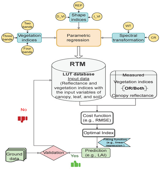
Figure 2.
Workflow diagram of parametric algorithms in the hybrid method.
2.1.1. Vegetation Indices
Vegetation index (VI), which was developed in the 1970s, is a mathematical combination of surface reflectance from multiple bands to refine information about canopy attributes, reducing susceptibility to confound influences such as soil background, illumination geometry, and atmospheric conditions [57,58,59]. The observations from several spectral bands are transformed to provide a single value of VI. These numerical transformations, which are semi-analytical measurements of vegetative activity, have been shown to differ considerably not just with seasonal variation in green foliage but also throughout space, making them valuable for identifying within-field spatial variability (i.e., in precision farming application) [60].
VIs can be calculated from either broadband spectra (more than 50 nm intervals) or narrowband spectra (5–10 nm intervals) [61,62]. In broadband VIs computed from multispectral data, VIs intend to study the spectral properties of vegetation in both the visible and near-infrared regions of the spectrum. The spectral response of vegetation within the red domain is powerfully related to the amount and concentration of photosynthetic pigments such as chlorophyll concentration, whereas the spectral response within the near-infrared region is controlled by leaf structural characteristics (e.g., LAI and fCover). Since hyperspectral narrow band data can separate and characterize the canopy, narrow-band vegetation indices are recommended for use by finding the most effective combination between spectral bands. Many VIs have been developed moving from two bands (e.g., Normalized Difference Vegetation Index (NDVI)) toward four spectral bands (e.g., the transformed chlorophyll absorption in reflectance index/the optimized soil adjusted vegetation index (TCARI/OSAVI)) [63]. The accuracy of estimates using VIs as model inputs can be affected if the study does not identify an appropriate index through model inversion [64]. Further information about this technique presenting the general concept of VIs can be found in these studies: [65,66,67] for LAI, ref. [68] for fCover, and [69] for CC.
2.1.2. Shape Indices
As an alternative to classical VIs, shape indices have been investigated to enhance absorption features present in vegetation spectra since the advent of hyperspectral data. One of the most common calculations used in the category of shape indices, the red edge position (REP), is a significant feature for detecting the variations of crop variables [70,71,72]. It is defined as the maximum first derivative of the spectrum between the red and NIR domains [73,74]. This region was often used to infer crop characteristics such as LAI and CC [75,76]. Recently, it was discovered that the indices created by the red edge (RE) bands (680–780 nm) are useful to enhance the precision of the estimates [76,77,78,79]. The extraction of REP parameters from various sources of spectral data has resulted in the development of a number of techniques, such as maximum first derivative (MFD) [80,81], the polynomial fitting (PF) technique [82], the inverted Gaussian (IG) technique [83], and the linear extrapolation (LE) technique [84]. Cui et al. [85] succeeded in increasing the accuracy of predicated LCC by proposing a new VI called red edge chlorophyll absorption index (RECAI) and integrated it with classical VI (TVI).
Besides REP, there are other methods of calculation indices that depend on the derivative-based VIs (D_VI) and integration (I_VI) [86]. Both methods convert the original spectrum band for any spectral region, including the red edge band, into an index. In the D_VI, the slope and first and second derivative curves of spectral reflectance are determined instead of using reflectance values, while in the I_VI, the integration of the spectral regions at the visible wavelengths and the red edge is used to normalize the vegetation index. Further details can be found in [72,87,88,89]. Indices based on derivative spectra have been demonstrated to be more successful than reflectance-based indices because they principally reduce background signals and separate overlapping spectra using a variety of differentiation techniques [61]. Some studies performed a systematic evaluation between conventional VI and derivative-based indices, and the results confirmed that it is not necessary to see such improvement when using a derivative-based index [86,90]. In the study of [91], the double-peak nitrogen index (DCNI I) was the best for estimating chlorophyll content, resulting in the ability to assess nitrogen content. For LAI, Qiu et al. [92] constructed new derivative parameters of NDVI to improve the estimation accuracy. Compared to the derivative-based index approach, the integration-based indices are utilized for retrieving leaf chlorophyll (LCC) [89,93,94].
2.1.3. Spectral Transformations
In addition to the previous techniques, continuum removal and wavelet transform methods are developed for airborne or satellite hyperspectral imaging instruments. Kokaly and Clark [95] tested the potential of continuum removal (CR), a technique that is frequently employed in geology, using dried leaf specimens, where broad absorption characteristics in dry leaf spectra were subjected to CR, and absorption-band depths in relation to the continuum were computed. Each absorption feature’s band depths were normalized. The depth at the feature’s center and the region under the band depth curve were used to examine normalization. In other words, CR normalizes the reflectance spectrum by comparing different absorption properties related to vegetation characteristics with a common baseline [96,97,98]. For instance, in the study of [99], the Chlorophyll Absorption Continuum Index (CACI) was developed and calculated, based on computing the area under the spectral curve between 550 and 730 nm. Other studies also used this technique for enhancing the accuracy of crop traits (LAI, nitrogen, and chlorophyll) [97,100,101]. The wavelet transform (WT) method is a viable method for analyzing the spectrum that converts the original reflectance spectrum into coefficients resolving at high scales (e.g., small narrow bandwidth absorption features) and low scales (e.g., broad absorption features). The discrete wavelet transform (DWT) and the continuous wavelet transform (CWT) are methods utilized to extract spectral features, whereby using one of these methods, the optimum number of wavelet coefficients associated with a particular type of spectral feature is determined [102]. Different studies focus on the WT method for estimating LAI [103,104], chlorophyll content [105,106], fCover [107], and nitrogen [108].
2.2. Hybrid Approach Based on Nonparametric Methods
The nonparametric methods have recently gained prominence in the era of free Earth observation (EO) data streams. In practice, the LUT databases, including pairs of simulation and canopy parameters, are used to fit linear or nonlinear nonparametric regression formulas, and the fitted equation is then utilized for estimating land surface parameters. This is performed after the training data and testing data have been prepared. This is a critical step for developing generic and robust hybrid models and is a typical application of the supervised learning model. The learning process successfully lies in the ability to minimize the error of the training sets and improve the accuracy over iterations [109]. To assess the generalizability of the regression model, the model should be tested based on independent (unseen) datasets to ensure full interpretation of the spectral variance in the optical remote sensing image that is reflected in the accuracy of the plant characteristics of interest. Lastly, the results (estimated canopy characteristics of interest) from the successful trained model should be validated with the ground data (Figure 3). Table 2 displays the advantages and limitations and caveats of the nonparametric method.
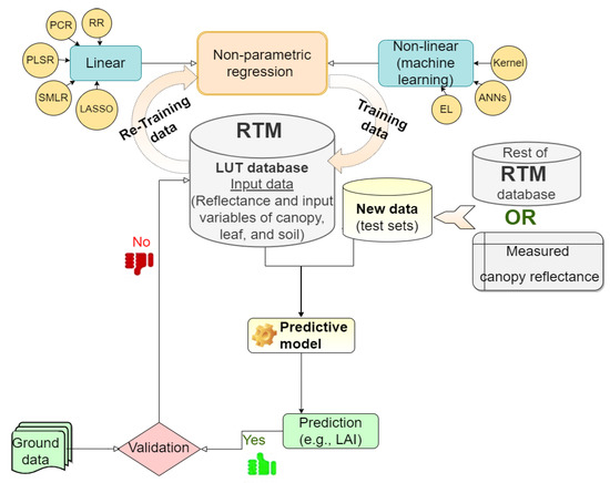
Figure 3.
Flow chart of nonparametric algorithms process in the hybrid method.
Table 2.
Summary of the advantages and limitations and caveats of the nonparametric method.
2.2.1. Linear Nonparametric Regression Methods
Linear regression applied to optical data deals with more than one single explanatory variable, called a regressor (X), for a regression model to determine the response variable (Y) while keeping the assumption of linearity. Stepwise multiple linear regression (SMLR), principal component analysis (PCA), and partial least square error (PLSR) are the most popularized methods used in the 1980s, as compared to ridge regression (RR) and least absolute shrinkage and selection operator (LASSO). These methods have been adopted from simple linear regression. Table 3 presents the comparison of pros and cons of different model representations.
- Stepwise multiple linear regressionStepwise multiple linear regression (SMLR) is a way to select the most significant explanatory variable from a set of independent variables that has the highest correlation with the response variable (Y) [110]. The SMLR method is conducted in two phases: forward and backward stepwise selections. The model starts with no variable (spectral bands) and adds variables one by one, which is the most significant part. Then, a backward elimination procedure starts with all spectral bands and removes the bands one-by-one, obtaining the least statistically significant. Typically, the range of the p-value for entering and removing the variables is set between 0.01–0.02 [58]. In addition, to quantify the severity of multicollinearity between explanatory variables, the variance inflation factor (VIF) is an index to measure how much variance there is of the estimated regression coefficient. A rule of thumb is that if VIF is more than 10, then the data have high collinearity [111], otherwise no collinearity between independent variables is found.
- Principal component regressionPrincipal component regression (PCR) is based on a combination of principal component analysis (PCA) and linear regression model [112]. The main idea is to convert the original variables into a new set of synthetic variables, which are independent of each other. By using a linear transformation, the data are transformed into a new orthogonal coordinate system where the data with the largest variance are displayed on the first axis (referred to as the first PC), the data with the second-largest variance on the second axis (referred to as the second PC), and so on [98]. As a result, the orthogonal PCs are ordered from the highest to lowest variance data information of spectral features.
- Partial least square regressionFollowing a similar idea to the above method, partial least square regression (PLSR) relies on two methods, which are PCR and canonical correlation analysis (CCA). A large number of correlated variables of the spectral data is reduced to a few non-correlated variables, with high variability. For the case of PCR, the projection space of PCA depends only on the independent data (X); however, in partial least squares (PLS), the projection space of X is explicative of both X and Y. The original variables X and Y are transformed into their respective latent variables (X1 and Y1), and then PLS seeks the most probable linear correlation between latent variables (the idea of CCA).
- Ridge regressionRidge regression (RR) is a method for estimating the coefficients of multiple-regression models in scenarios with highly correlated linearly independent variables. A new trendline is introduced to fit the training data by adding a certain amount of bias in the regression estimates to obtain reliable approximations of the population values. The bias called lambda () plays a role to control the trade-off of bias variance and the user tries to find the best value of lambda that has low variance using cross-validation. With increasing lambda value, the important parameters may shrink to be zero, and fewer stay at high values.
- Least absolute shrinkage and selection operatorThis approach, abbreviated as LASSO, uses variable selection and regularization to improve the statistical model’s prediction accuracy and interpretability. This method allows forcing the most and least important parameters to be close to zero or absolute zero, as compared to RR.
Table 3.
Pros and cons of the linear nonparametric methods.
Table 3.
Pros and cons of the linear nonparametric methods.
| Methods | Pros | Cons |
|---|---|---|
| SMLR | (1) Simple, fast, and easy to use. | (1) Suffers from multicollinearity when applied to canopy hyperspectral data. |
| (2) Screens a large number of potential predictors to obtain the best one. | (2) The selected wavelength is often not related to the absorption characteristics of the compounds of interest [113,114]. | |
| PCR | (1) Mitigates multicollinearity and avoids overfitting problem. | (1) Does not consider the response variable (Y) when deciding which principal components are dropped and relies only on the magnitude of the variance of components. |
| (2) Improves the predictive performance and provides stable result in regression coefficient. | (2) Does not perform feature selection. | |
| (3) Issue of interpretability. | ||
| PLSR | (1) Handles multiple inputs and outputs, data noise, and missing data. | (1) Relies on the cross-product relations with the response variables and is not based on the (co)variances between independent variables. |
| (2) Has difficulty explaining. | ||
| (3) Response distribution unknown. | ||
| RR | (1) Solves the problem of overfitting. | (1) Low in-model interpretability. |
| (2) Adds bias to estimators to reduce the standard error. | (2) Unimplemented the feature selection. | |
| (3) Uses all the predictors in the final model. | (3) Trades the variance for bias. | |
| LASSO | (1) Performs feature selection. | (1) Arbitrarily selection. |
| (2) Fast in terms of inference and fitting. | (2) Difficult to justify which predictor needs to select. | |
| (3) Avoids overfitting. | (3) Uses a small bias in the model since the prediction is too dependent upon the particular variable. | |
| (4) Lower prediction performance than RR. |
2.2.2. Nonlinear–Nonparametric Methods: Machine Learning
As a part of the retrieval methods used in the hybrid model, machine learning (ML) does not rely on any particular form of the regression function to characterize the connection between the dependent (variable of interest) and explanatory variables (in this case, a spectral reflectance image). In addition, ML not only provides a powerful and flexible framework of the data-driven method for making a decision, but it also allows for the incorporation of expert knowledge into a learning system. For this reason, ML is becoming increasingly popular and important in the field of agricultural monitoring studies. Below is a brief description of ML methods, with their pros and cons summarized in Table 4.
Table 4.
Pros and cons of nonlinear nonparametric methods.
- Artificial Neural NetworksAn artificial neural network (ANN) is a collection of connected artificial neurons, and each artificial neuron or node connects to another, linking with weight, and nonlinear equations are specified by the activation function (e.g., rectified linear unit or sigmoid functions). Through a nonlinear function of the sum of its inputs, the output of each neuron is calculated. When exceeding a certain value of the threshold/activation function of the output node, then the node is activated and data are sent to the next layer (having a set of neurons or nodes) of the neural network, known as the hidden layer [115]. This leads us to identify the design or structure of ANN starting from simple to the complex one, depending on the number of hidden layers, the number of artificial neurons, the directional flows (uni or multi), the type of activation function used, and how many inputs and outputs are used in the model. An example of simple architecture is a feed-forward neural network (FFANN). It was often used in remote sensing for mapping vegetation properties in the mid-1990s. This is a unidirectional flow, where the information from the input nodes is transferred to the output nodes.An back-propagation neural network (BPANN) is built based on using multi-directional forward and backward mode and the error rate obtained from the output layer and distributed back through the network layers [116]. As an alternative to the aforementioned methods, radial basis function (RBFANN) [117], recurrent neural network (RANN) [118], and Bayesian regularized ANN (BRANN) are advanced models that deal with a large quantity of remotely sensed data [119].Deep neural networks (DNNs), which emerged in 2015, have achieved excellent results in classification tasks. Nevertheless, DNN is still under investigation for regression in experimental and operational hybrid settings [24]. It uses many hidden layers and relatively few neurons per layer, as compared to the simple structure of NNs [115]. Ultimately, the success of NN performance relies on how the user adjusts the hyperparameters, such as the number of hidden layers and neurons in the layer, to minimize the difference between the model prediction and the desired outcome, respecting a good trade-off between the computational time, stability, and accuracy [34].
- Ensemble learningEnsemble learning (EL) uses multiple learners that are trained to solve the same problem. The EL approach mixes numerous decision trees to generate higher predictive power, instead of using a single decision tree. Bagging and boosting are the main families of ensemble methods. An ensemble is made up of a group of learners known as base learners. An ensemble’s generalization ability is usually much higher than that of base learners.- The bagging technique is the short form for bootstrap aggregating, in which the independent multiple sub-groups of features are randomly created with iterative replacement from original training datasets. Their decision trees are trained with each group of data and aggregated to average (reducing the variance of the decision tree) to obtain the final prediction [120].Random forest regression (RFR) is an extension over bagging where a subset of features is randomly selected from the total and the best split feature from the feature subsets is used to split each node in a tree and all features are examined for splitting at a node [121].A canonical correlation forest (CCF) is a collection of decision trees that are constructed by several canonical correlation trees (CCTs). They are trained by using canonical correlation analysis (CCA) to determine feature projections providing the maximum correlation between features and then picking the optimal splits in this projected space. The results from individual CCTs combine to make a final prediction for unknown samples [122]. Contrary to RF, CCF uses full training datasets in selecting split points at each tree. Since the bagging approach works based on the combination of multiple weak learners to obtain a stable result, it is the preferred method to be used for any study. However, the result can be biased if the model is properly adapted and thus may result in underfitting.- Boosting is a dependent framework, based on generating several weaker learners in a very adaptable manner and sequentially to make a strong learner. At every step, a new model is built upon the previous one to boost the training instances by weighing previously mislabeled examples with higher weight. The best example of a dependent framework is gradient boosting regression tree (GBRT), introduced by [123], which aims to reduce the bias rather than variance. On the other hand, random forests reduce the variance of the regression predictions without changing the bias.
- Kernel machinesA kernel machine uses a kernel to perform calculations in a higher-dimensional space without explicitly doing so. Kernel methods transform data from their original location (known as input space) to a higher-dimensional space (known as feature space). Then, in the feature space, these approaches look for linear decision functions that become nonlinear decision functions in the input space [124]. Kernel methods replace the inner product of the observations with a chosen Kernel function. There are various classes of kernel functions, including the linear kernel, radial basis function, polynomial, and sigmoid functions. They should be continuous, symmetric, and have a positive definite value.- Support vector regression (SVR) was introduced in the late 1990s to early 2000s by [125,126] SVR enables the extraction of the complex nonlinear relationships between the feature vector (X) containing spectral information and the variable of interest (Y) using the kernel trick. This approach determines how much error is acceptable in the model and finds an appropriate line (or hyperplane) to split the data spatially in high-dimension space. Ultimately, the performance of SVR depends on which kernel function is used in the model and how the user tuned their hyperparameters (epsilon-insensitive zone () and regularization (C) parameters). The parameter () controls the width of the epsilon-insensitive zone for the training data, whereas regularization (C) controls the trade-off between the minimization of errors and the regularization term [127].- Gaussian processes regression (GPR) follows the Bayesian theorem by using the probability distribution across all admissible functions that fit the data [128]. After specifying the prior on the function space, the posterior distribution is computed based on the prior distribution for the successor retrieval procedures [129]. Since GPR can describe the properties of functions, the mean of a (Gaussian) posterior distribution and variance are predicted. To increase the efficiency of the GPR model, the kernel’s hyperparameters (mean and covariance function) need to be tuned efficiently for maximizing the log-marginal likelihood in the training data [130].- Kernel ridge regressionKernel ridge regression (KRR) combines the kernel trick with ridge regression [19]. The key idea is that nonlinear map data can be transformed to high-dimensional feature space and linear regression embedded in feature space using a weight penalty. As a result, it learns a linear function in the space caused by the kernel and data. This relates to a nonlinear function in the original space for nonlinear kernels [131]. The model learned by KRR has the same form as support vector regression (SVR). The loss function of SVR is based on -insensitive loss with ridge regression, but KRR uses the square error loss function to solve a convex quadratic programming problem for classical SVMs [132].
3. Techniques Used for RTM Database in Hybrid Retrieval Strategies
To generate a lookup table database (LUT), all possible combinations of canopy variables are produced by defining the boundaries and distributions of input parameters for a given model. This information can be acquired through the user experience, fieldwork, or/and previous studies [133]. Due to the large set of simulations stored in the LUT database (containing canopy parameter checks and their corresponding simulated spectra), various techniques have been proposed to help find the best spectral sample from the pooled dataset. The selected sample should contain sufficient and rich information to represent the objective under consideration. Neglecting this procedure may affect the accuracy of the estimated variable (Figure 4).
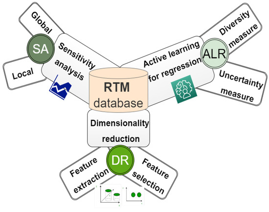
Figure 4.
Overview of the techniques used in simulating the data.
3.1. Calibrating the Lookup Table Inputs Based on Global and Local Sensitivity Analysis
Calibration of the model inputs before applying the RTM for a specific crop is an indispensable step since the model’s resilience and realism can be examined to improve the results. This is performed by minimizing the number of free variables [134]. For instance, the advanced RTMs (e.g., DART and SCOPE), which contain a great number of input parameters to characterize the complex land–atmosphere interactions in geophysical parameters, typically need intensive work for calibration. Indeed, some of the input parameters have a high impact on the model’s output, whilst others do not. Therefore, the role of using sensitivity analysis (SA) is attempted to identify which parameter is the most or least significant in a specific spectral region to understand the model process and quantify the uncertainty of each of them on the model output [135]. Each model input parameter is variated one at a time (OAT) in the model output, while the rest of the parameters remain constant at their central values. It is a straightforward technique belonging to a local SA. Such a sensitivity computes through gradients or discrete partial derivatives of spectrum reflectance while taking into account the input parameters [136]. Regarding its simplicity and inexpensive computational time, it is often used, although it is not suited for complex models and does not know the interaction between parameters. To overcome this drawback, global SA (all at a time (AAT)) has been explored to present the variations in the model input parameters individually (first-order effects) and collectively through their interactions (known here as the total-order effects). This can create the variability of the model output [137,138]. Besides applying GSA to the input parameters of RTM, the GSA of VI based on RTM simulations is carried out to evaluate the propagation of uncertainty obtained from confounding factors (e.g., soil background and atmospheric correction). It may lead to improvements in the results of using VI to describe canopy properties [138,139].
In general, here are some of the most commonly used techniques in global SA:
- Variance-based sensitivity analysis (VBSA), such as the Sobol method [140], Fourier amplitude sensitivity test (FAST), and the extended Fourier amplitude (EFAST) [141,142,143,144].
- Density-based sensitivity analysis (DBSA) [93,137,145].
- Global screening method, such as the Morris method [146] and Latin hypercube-OAT (LH-OAT) [147].
- Regression/correlation-based techniques [148].
- Regionalized sensitivity analysis (RSA) [149].
In RTMs (e.g., PROSAIL, SLC, and SCOPE), several studies have widely applied the VBSA [63,135,138,150,151], rather than the DBSA [152], method. The VBSA aims to quantify the variance of the main effect and the higher-order effect of factors that contributed to the variance of the model output [63]. Instead of using variance as a basic assumption of VBSA, DBSA analyzes the distribution of model output using probabilities density function (PDF) or cumulative distribution function (CDF) of the output to characterize its uncertainty [152].
3.2. Active Learning for Regression Tasks
The experimental design and sampling strategy play important role in the retrieval process as the size of the LUT has an impact on the accuracy of the estimates. With a small size of the LUT, the estimation accuracy can deteriorate. Contrarily, the large size might lengthen computation times without providing any additional benefits in terms of accuracy [153]. The goal of experimental designs is to maximize the information from a small number of simulations [154]. From here, the role of ML can be accessed. A form of ML known as “active learning (AL)” allows learning algorithms to engage with users to categorize data with desired outcomes. AL can be used for classification, emulation, or regression task [155]. In hybrid retrieval schemes, ALR is a subclass of an intelligent sampling methodology for active learning (AL), known as “optimal experimental design”. It is an alternative approach to random sampling strategy [155]. It is a naive approach and may not lead to optimal sample selection [156]. Hence, this approach is modified by the introduction of systematic sampling and stratified sampling. This refers to Latin hypercube sampling (LHS) as an effective method for sampling from their multivariate distributions [157].
Returning to ALR, the objective of this method is to reduce the sample size of the pooled dataset while having the richness and diversity of information [156]. Through the regression process, a number of labeled samples are needed to build a regression model with good generalization ability [158]. In a hybrid scheme, a large database generated from RTM consists of unlabeled samples. This means that we cannot know which of the reflectance spectra belongs to which set of input parameters, and it may not be useful to use them all for training via advanced regression methods (e.g., kernel methods and deep learning) [159,160]. Most of these databases contain quite redundant information and are noisy, leading to high computation time and dispersion of estimates [161]. Therefore, the need for ALR in data classification is an indispensable task to solve the problem of training a sample collection. Theoretically, ALR starts with selected small training datasets of label data and then repeatedly adds new samples to the original training set of samples (unlabeled data), depending on query criteria. This can be defined by either uncertainty [162] or diversity measures [163], without involving human experts. An uncertainty query aims to find unlabeled samples, which are the most uncertain instance with the least confidence near the decision boundary. The selected samples are used to delimit the position of boundary decision and then labeled to include them later in the training set and remove them from the candidate test [164].
There are two known measures that have been used to obtain a reliable sample. The first measure is the calculation of uncertainty when sampling ALR. This is roughly divided into three categories, as follows: a variance-based pool of regressors (PAL) [165], entropy query by bagging (EQB) [166], and residual regression AL (RSAL) [167]. In the second measure, for taking a diversity of unlabeled samples, which depends on the diversity or the distance between the samples, the selected samples are added to the training data after labeling them. Thus, the redundancy among the selected samples is avoided [168]. In this measure, three classes are used: (1) Euclidean distance diversity (EBD) [169]; (2) angle-based diversity (ABD) [168]; and (3) cluster-based diversity (CBD) [170].
To obtain more knowledge about AL heuristics, the study of [171,172] is elaborated in detail. Several studies have been devoted to evaluating six types of two measures of AL with kernel methods (GPR and KRR) using multispectral and hyperspectral data [155,159,171,173,174]. They were unanimous that the diversity measure (especially EBD) outperformed the uncertainty measure, because it delivered the highest levels of accuracy while speeding up the time required for computation [155].
3.3. Curse of Dimensionality
With the increasing dimensionality of spectral features, the data become increasingly sparse in the space they occupy. This case typically occurs in the hyperspectral data, which oversample reflectance spectra in many wavelengths, leading to multicollinearity between spectral bands. In addition, processing such a big data stream is going to degrade regarding the heavy computational burden and storage cost. Therefore, dimensionality reduction (DR) has to be taken to tackle the curse of dimensionality (CoD) problem by condensing or reducing the spectral data while preserving the significant information in the original data. In the context of a hybrid retrieval processing chain, using DR with nonparametric regression to train the LUT database becomes a favorite step for improving the accuracy of canopy retrievals while gaining some speediness in the processing [175]. These simulations with high-dimensional data can be redundant information and need to be condensed to significant information content to have a low dimension space. Another issue of CoD is overfitting, where training (sparse) data by using the advanced regression models could lead to an increase in variance. This is because the model repeatedly performs the training process during the calibration process to reach the best results. However, when applying the model to unseen data through the validation process, the estimation accuracy is decreased.
Two techniques are commonly applied to tackling such a problem (CoD): feature extraction and feature (band) selection. Feature extraction (FE) is the process of transforming information from an original feature dataset into an appropriate new feature subspace. Such a technique can reduce the model complexity and generalization error introduced by noise irrelevant to features. Among feature extraction methods, PCA [176] and PLS [177] are the most popular methods in chemometric and remote sensing applications.
With the second technique (feature (band) selection) (FS), the original feature of spectral bands is subsetting into small feature sizes by removing the redundant or irrelevant features. In other words, the original representation of the data is not altered and maintains the original meaning, unlike feature extraction. From a practical perspective, the feature band selection is categorized into three groups: the filter, the wrapper, and the embedded techniques. Compared to the embedded method [178], filter [179] and wrapper [180] band selections are major methods used in the field of remote sensing, especially in classification tasks; however, less work focuses on retrieval studies [174].
- Filter approach is extracting and ranking the spectra features as a preprocessing step before learning the algorithm [181]. The best feature with a high rank is chosen and the redundant or irrelevant features are filtered out. This can be performed by finding the highest correlation between a spectral feature and a dependent variable. The vegetation index (VI) is a typical case for the filter method [174]. Before applying regression, all possible band combinations between two or three bands through generic VI-based LUT datasets are regressed against the targeted variable. The model’s performance is assessed based on the determination coefficient as a measure.
- Wrapper approach uses a predefined learning algorithm to search the space of all possible subsets of features. The most informative spectral features based on their predictive performance are selected for retrieving canopy properties. This process is repetitive to improve the performance of the previously selected feature subset [182]. Some methods belong to this group, such as recursive feature elimination (RFE) [183], simulated annealing (SA) [184], genetic algorithms (GA) [185], and correlation-based feature selection (CFS) [186]. Moreover, nonparameter linear or nonlinear algorithms (e.g., SMLR, PLSR, RFR, and GPR) are capable of feature selection as well as regression [58,187]. These strategies have been used in different studies to determine the best band settings for retrieving biochemical and biophysical characteristics from hyperspectral data [23,188].
- Embedded method is the last group of FS, which is an extension of the wrapper method, except that the training data do not need to be split into training and test sets [189].
4. Systematic Reviews
In this section of the reviewed articles, each of the three variables of interest is classified into two categories; one for the parametric method and the other one for the nonparametric method. To screen the literature review for such an objective, Scopus, Google Scholar, ScienceDirect, PubMed, Web of Science, and MDPI were used as search engines. In addition, the “hybrid retrieval method” was used in conjunction with each of the following keywords: “machine learning, vegetation indices, radiative transfer model, LAI, fCover or vegetation cover, and LCC and CCC”. A total of 102 publications were found in total for 2000–2022. On the other hand, publications in languages other than English, conference papers, chapters, reviews, and master’s and doctoral theses were excluded after reviewing the aggregated data for the published papers.
Finally, 73 of the total published papers, which include 46 and 27 papers applied to nonparametric and parametric methods, respectively, were identified under this research. Figure 5 shows the general trend of published papers over a period of 22 years, indicating the greater use of the hybrid retrieval approach in the journal Remote Sensing rather than the journal Remote Sensing in Environment. Moreover, the upper part of Figure 5 shows that there is a larger number of publications applying the nonparametric method for training the LUT database (64%) than the parametric method (36%).
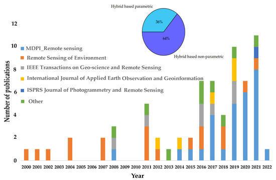
Figure 5.
(Lower part) Bar chart showing the number of studies versus the annual number of published papers in different journals from 2000 to 2022. (Upper part) Pie chart showing the percentage of published papers applied for nonparametric compared to parametric methods based on the radiative transfer model (RTM) approach.
4.1. Estimated Canopy Traits from Hybrid Models Based on Parametric Methods
4.1.1. Leaf Area Index
Two studies were devoted to analyzing the wheat crop. For example, the study of [190] explored the effect of using prior knowledge relating to the distribution in the LUT-based inversion. Moreover, by using fifteen vegetation indices along with the reflectance bands, the accuracy of leaf area index (LAI) winter wheat retrieval with different phenological stages was improved. In the other study [191], the authors also investigated the performance of reflectance-based LUT and vegetation index (VI)-based LUT over six experimental plots from 2018 to 2019 for wheat LAI retrieval.
For mixed crops including wheat, the red-edge-based VI was assessed from multitemporal RapidEye images and compared with VI-visible reflectance using synthetic spectrum [76]. The authors of [192] tried to find the optimal VI from nine tested VIs, using the curve fitting and backward feature elimination method (BFE) integrated with RFR. Then, three regression models, including curve fitting, k-nearest neighbor (KNN), and RFR, were determined to find the optimal algorithm for building the relationship between LAI and VIs. The aim of [193]’s study was close to the idea of other studies by finding the suitable LAI-VI that can be resistant to chlorophyll content and atmospheric and soil brightness effects. Concerning the property of generalization, the uncertainty measures were also considered through the analysis, which was mainly focused on the crop reflectance model (e.g., PROSAIL). As sources of propagation of uncertainty in LAI estimation, the influences of changing the solar zenith angle and atmospheric perturbations were tested over multiple years (1999 to 2006) and on a regional scale [194]. These authors focused on four indices (NDVI, OSAVI, EVI, and MTVI2) to show the spectral resolution under these conditions. Finally, Broge and Leblanc [99] carried out a systematic and rigorous evaluation between broad-band and narrow-band VIs to find out which of them could increase the accuracy of the estimation.
The authors of [195] dedicated their study to evaluating the performance of 43 hyperspectral VIs to find the optimal one based on two datasets of PROSAIL simulations. It also relied on prior knowledge of one from literature and the other from ground data. To build the relationship between LAI and simulated VIs, the simple (curve fitting) and advanced regression (RFR and ANN) models were employed. The same authors extended this study by comparing the results obtained from using 26 VIs and PLS dimension reduction with the use of appropriate principal components as the input variables for modeling inversion strategy [64]. Houborg et al. [196] evaluated the performance of a hybrid model based on VIs for mapping LAI over time and space. Under different spatial resolutions (250–500 m) for 8 days, the MODIS data were used in the coupling of PROSPECT and the two-layer Markov chain canopy reflectance (ACRM) model inversion. Moreover, in this study, a hybrid inversion scenario was investigated based on the combination of the measurements from the field and physical model. The target property (LAI) and explanatory variables of vegetation indices using Landsat 8, which were classified into five groups, were trained by using random forest and cubist regression approaches. Table A1 summarizes the above papers and presents the main result for the LAI hybrid parametric method.
4.1.2. Fractional Vegetation Cover
In this category, few articles are reported to belong to hybrid spectral indices. The studies of [13,197] are mainly focused on improving such a variable of interest. In particular, the authors of [197] developed the physical model by considering multi-angle reflectance and LAI products to quantify the Normalized Difference Vegetation Index of highly dense vegetation (NDVIv) and bare soil (NDVIs) at coarse resolution (e.g., 1 km) for estimating fCover. The other study [13] proposed a method called the “fan-shaped method” (FSM) to mitigate the effect of CCC variation in the pixel dichotomy model (PDM)-based FVC estimation. For fCover estimation, an FSM method, which creates a two-dimensional scatter map with three vertices, represents high and low levels of CCC values, and bare soil using a CCC spectral index (SI). It relied on spectra simulated on PROSAIL and spectra measurements delivered from UAV. Lastly, the studies of [198,199] evaluated the impact of soil background and leaf angle distribution (LAD) on fCover estimation by using a set of different vegetation indices. Table A2 summarizes the above papers for the fCover hybrid parametric method.
4.1.3. Chlorophyll Content at Leaf and Canopy Levels
For corn, Haboudane et al. [69] integrated a new index by combining two indices as a ratio TCARI/OSAVI. It has the potential to predict CCC and minimize the background and LAI effects. Another study by [200] studied the effects of different nitrogen fertilization with eight levels on CC estimation for corn. Two spectral indices (MCARI and OSAVI) were combined with spectral bands, such as OSAVI and NIR/red and MCARI and NIR/green, to define which indices can minimize the background and are sensitive to LCC. In the last study [201], two cultivars of corn were planted in the field experiment; spectral features based on vegetation indices, wavelet coefficient (WC), and spectral reflectance were assessed for estimating the LCC.
Three articles are reported for potatoes. In the study of [202], a systematic evaluation between sets of VIs was determined to define the suitable VI for estimation of canopy chlorophyll content (CCC). The authors of [38] hypothesized that using the ratio of vegetation indices based on LAI normalization can accurately estimate leaf chlorophyll content (LCC) by mitigating the other external factors (e.g., soil background properties, changing leaf orientation, or changing solar zenith angle). The simulated spectra were evaluated with field measurements for five consecutive years between 2010 and 2014. The last article [36] studied fifty hyperspectral vegetation indices for potatoes, where indices were tested to retrieve LCC and CCC. To verify the inversion result, observed data, including auxiliary data obtained from fieldwork and CHRIS image data, were utilized.
As shown from the presented systematic reviews (Table A3), two articles [201,203] devoted their analysis to wheat. The authors [201] suggested a new strategy to improve LCC estimation by building a matrix-based VI combination for minimizing the influence of LAI. Single VI (e.g., MCARI and OSAVI) and the ratio of VIs (e.g., red edge relative index) were used to build a matrix of two VIs (VI1–VI2) space and each cell of the matrix was assigned to an LCC value using simulated data. For the study of [203], the extracted wavelengths of LCC were selected by the amplitude- and shape-enhanced 2D correlation spectrum based on using PROSAIL. Deep learning was then utilized for training the PROSAIL database to the inversion tasks of field-measured LCC.
Several studies cultivated different crops in the field, such as wheat, corn, and soybean [204,205,206,207]. These studies tried to increase the sensitivity of VI to chlorophyll content variations and resistance to LAI and other permutation factors (such as soil background). Particularly, ref. [204] concluded that the type of crop, the type of data obtained from model simulations or/and from field measurements, spectral range, and model type can influence the predictions of variables. Table A3 summarizes the results from the aforementioned papers.
4.2. Estimated Canopy Traits from Hybrid Models Based on Nonparametric Methods
4.2.1. Leaf Area Index
The study of [208] proposed a new approach to alleviating the ill-posed problem that relies on the use of the object signature for a specific crop. The synthetic database was built based on the spectrum signature obtained from a neighboring pixel of interest using a neural network. The authors proved that the suggested method can reduce the uncertainties in estimations and does not require the use of prior knowledge for constraining the boundary of input parameters or identifying the crop type. Another study [209] attempted to solve the inversion problem by introducing SVR-based kernel regularization to reduce the number of simulations, leading to reduced computational time, rather than using NN, which requires a large number of datasets for training. The recent article [52] introduces the variable correlation through the generation of LUT to produce a realistic simulation from accurate representative combinations of the input parameter. The regularized LUT (LUTreg) was trained by GPR-based kernel since it performs well due to the unnecessity of using a large size of datasets with robustness in the estimation along with providing the uncertainty of estimates. In the article [210], the authors explored the utility of active learning (AL) with a GPR method to train simulated datasets for reducing the sample size and redundant information. To study its performance, the outcome was compared with the results of non-kernel methods for a specific crop (wheat). By applying the hybrid NN model for the same crop at different growing seasons, the study of [211] intended to optimize this approach by decreasing the uncertainty of LAI estimation, especially when values of LAI or green leaf area index (GLAI) are high due to the saturation effect.
Other studies for such a corn crop [187,192] were devoted to finding the optimal method based on a comparison of different retrieval methods. The same objective was applied to the study of [212,213]. With the availability of multiple data sources from multiresolution satellite data, a hybrid model can help to create a generic model, transferable and independent from in situ data, as shown in the study of [214]. Additionally, other studies [20,195] used Landsat 8 and SPOT 5 to confirm the robustness and consistency of the retrieval chain for monitoring the real spatiotemporal changes in crop development. Table A4 summarizes the above papers for a hybrid nonparametric method sub-category.
4.2.2. Fractional Vegetation Cover
Two studies [215,216] suggested the combination of the two models, RTM and crop growth model, for time series fCover estimation using a dynamic Bayesian network (DBN). It was generated from coarse-resolution remote sensing data and validated with a fine temporal and high spatial resolution. As shown from their findings, the proposed method gave reliable results and was visible for use at a large scale with various types of vegetation. Extending the previous two studies, a study of [217] utilized the proposed method based on GLASS FVC data from MODIS with temporal dependencies for each Landsat 7 ETM+ pixel to constrain the dynamic vegetation growth model. They concluded that the computational power of the proposed method was improved and feasible for real-time fCover estimation. A comparison between different nonparametric approaches was performed, and GPR was found to be the best algorithm using Sentinel-2 [210]. However, in the study of [52], RF was the best retrieval for fCover using UAV-based hyperspectral data.
Three studies [216,218,219] utilized a hybrid retrieval method for their study area with corn and wheat fields. In these studies, the authors were interested in quantifying the spatiotemporal fCover products from different scales of remote sensing. That needs, first, temporal consistency between remote sensing products to have a time series of fCover. Then, after training the simulation data by ML, the spatiotemporal fusion algorithm is used to make spatial consistency between RS data for improving the accuracy of fCover estimates. The last article [219] developed the hybrid framework using ML to retrieve the variable of interest from the bottom of the atmosphere (BOA) and the top of the atmosphere (TOA). The rest of the studies in Table A5 applied a hybrid retrieval model for the mixed plants. Table A5 summarizes the above papers and presents the main result of the hybrid nonparametric method.
4.2.3. Chlorophyll Content at Leaf and Canopy Levels
Several researchers studied wheat as one of the most common crops [210,220,221,222,223]. Two of the researchers were interested in studying AL techniques with GPR. Respecting the use of different sensors in these studies [210,222], entropy query by bagging (EQB) and Euclidean distance-based diversity (EBD) was the most efficient technique in terms of accuracy and computational demand. Indeed, the study of [210] intended to compare different regression methods for estimating LCC and CCC at two different locations and found that RFR and PLSR performed better than GPR + AL.
These findings are in agreement with other studies [52,224] when comparing GPR with other MLs. However, some studies, such as [206,219,225,226], preferred to place their attention on one method of MLs for increasing the efficiency of training RTM-based inversion to improve the accuracy of estimations. Another study [227] was dedicated to improving the sampling strategy in a simulated dataset to decrease the problem of ill-posed inversion. Different types of distributed datasets of simulations and variable relations were applied to reflect the real situation in the field. Other studies [201,221] compared NN and Bayesian network (BN) within a hybrid retrieval framework with LUT-based inversion, aiming to improve the accuracy of estimates. Finally, two studies [220,228] discussed the impact of different spatial resolutions on the vegetation variables and tried to decrease the uncertainties obtained from the model when applied to heterogeneous pixels. Table A6 summarizes the outcomes from the above papers for the CCC using the hybrid nonparametric method.
5. Results, Meta-Analysis, and Discussion
Based on analyzing the articles contributed in this arena, it was found that several researchers placed more attention on methods of hybrid-model-based nonparametric, specifically nonlinear, than parametric methods (Figure 6 and Figure 7). In a parametric method, most of the researchers often used vegetation indices for LAI, fCover, and CC, especially the Normalized Difference Vegetation Index (NDVI), which is extensively applied as compared to other indices such as the enhanced vegetation index (EVI), the modified triangular vegetation index (MTVI2 and MTVI1), the (optimized) soil adjusted vegetation index (SAVI and OSAVI), the chlorophyll index CIgreen or the red edge, the Transformed Chlorophyll Absorption Reflectance Index, and the Transformed Chlorophyll Index (TCARI and TCI) using satellite. There are a few researchers who, in their studies, used shape indices and shape transformation (i.e., red edge and waveform analysis). The results accuracy of estimates fall within the range R2 = 0.2–0.93 and RMSE = 0.05–0.94 m2/m2 for LAI, R2 = 0.54–0.90 and RMSE = 0.05–0.22 for fCover, R2 = 0.61–0.85 and RMSE = 3.24–11.90 (g cm) for LCC, and 0.61–0.85 and RMSE = 9.28–77.10 (g m) for CCC.
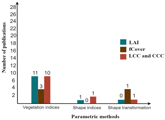
Figure 6.
Bar chart of the most contributed parametric methods in a hybrid model.
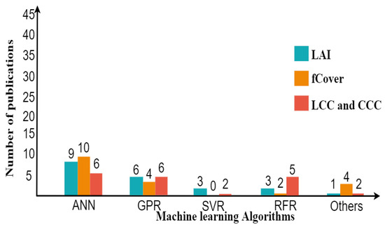
Figure 7.
Bar chart of the most contributed machine learning methods used in a hybrid model.
Within the various types of nonparametric methods, the hybrid model based on machine learning using ANN excels in improving the accuracy of estimates (Figure 7). Several studies applied machine learning more than the linear nonparametric methods (e.g., PLSR and LSLR), which only applied in two studies [133,210]. The accuracy of LAI ranges from 0.63–0.83 for R2 and 0.32–3.89 m2/m2 for RMSE. fCover’s accuracy ranges from 0.70–0.98 for R2 and 0.05–0.10 for RMSE. The accuracy of LCC and CCC falls within range for R2 = 0.38–0.93 and RMSE = 6.5–57.51 (g cm), R2 = 0.55–0.78, and RMSE = 0.35–111.90 (g m), respectively. When comparing the range of accuracy from two approaches, it was shown that the nonparametric approach was successful to obtain the best result for fCover rather than the parametric approach. In particular, nonparametric nonlinear methods are powerful in extracting information from subtle differences in reflection by supporting covariance between biochemical and biophysical variables [18].
Another remark is that after ANN, GPR is becoming more popular and applicable in the retrieval process, since Verrelst et al. [130] found that GPR had the best performance using Sentinel-2 and -3 and provides retrieval uncertainties (Figure 7). Nowadays, deep learning (DL), as extending machine learning, is starting to be explored for crop monitoring using hyperspectral images [34,229]. DL has the advantage of handling a large data size of training samples to possibly improve the targeted variable.
In the hybrid model context, the wheat crop was mostly analyzed by researchers, followed by corn, potato, soybean, and rice, as shown in Figure 8. Other crop types comprise grapes, barley, alfalfa, sugar beet, oil-seed rape, cotton, pea, sunflower, garlic, and onion.
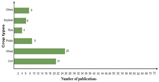
Figure 8.
The most investigated crops using hybrid inversion model.
From synthesizing the reviewed studies, PROSAIL, which is an integration of the leaf level PROSPECT model and canopy-level SAIL model, seems to be more favorably used with the methods of vegetation indices and machine learning rather than other types of RTM (SLC [41], SCOPE [230], and DART [231]) (Figure 9). This is due to its simplification in terms of model parameterization and that it is computationally inexpensive and free for users in various computer languages [212]. Nevertheless, radiative transfer models were used less often in the literature for investigating agriculture features as compared to the pure regression models [9]. While regression models can only estimate one variable at a time, RTM can infer a wide range of vegetation features in a single model.
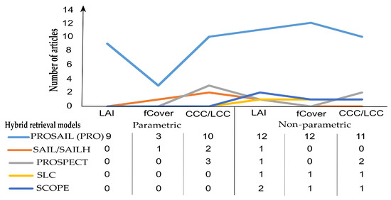
Figure 9.
Number of publications that used radiative transfer models within the period of 2000–2022.
Therefore, the next development of physical models should be simple and capable of generating a realistic simulation in the spatial and temporal dimensions for agricultural purposes. Analyzing such a large amount of remote sensing data necessitates a computationally efficient retrieval algorithm. Recently, some studies have tried to solve this issue by introducing emulation where a technique is used for estimating model simulations, such as RTM, to accelerate the inversion procedure and the speed of vegetation mapping [156,232].
Among the papers reviewed in this study, nonparametric approaches with multispectral data were employed in a hybrid model more than other platforms due to their accessibility (Figure 10). Nonetheless, hyperspectral data gathered from airborne platforms or drones have the potential to provide more precise spectral information regarding variables of interest, particularly in the red edge, NIR, and SWIR regions. Applying multisource remote sensing data, such as multispatial, multitemporal, and multiangular, in the framework of crop monitoring and management increases the estimation accuracy, as proved in these studies [20,54,130,233]. Limited access to high spectral resolution using a multisensor approach to regions of land cover heterogeneity at the pixel scale may cause the problem of scale effect. More studies need to explore approaches to eliminate the effect of size since many crops can grow together in one plot.
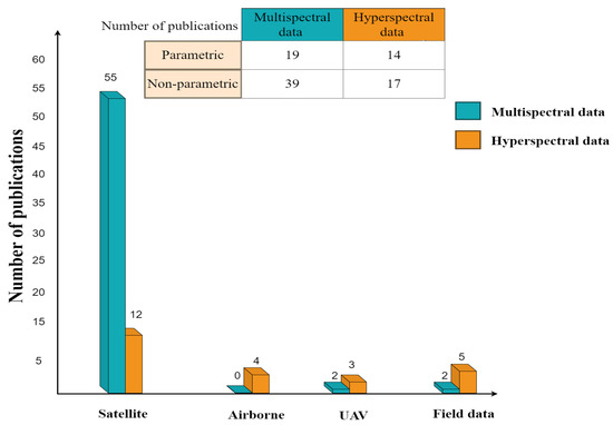
Figure 10.
Sensor type used in both categories of hybrid model.
6. Conclusions and Future Directions
In this review paper, we provided the conceptual framework of hybrid retrieval models and processing chains for retrieving biophysical and biochemical variables using parametric and nonparametric methods. In view of the increasing popularity of hybrid strategies, including machine learning, these methods may become a cornerstone in the context of precision agriculture applications and, in particular, for hyperspectral data processing.This popularity can be explained by the synergistic use of two complementary methods (data-driven and physical-based retrieval), which perfectly combines their advantages. The simplicity, flexibility, and computational efficiency of statistical methods are combined with the generalization capabilities of the physical-based method. Additionally, the need for collecting in-situ training data is reduced and used only for validating the targeted trait.
Upon the meta-analysis, we note that the NDVI-VI and NN algorithms have been extensively applied to Landsat and Sentinel-2 data, which are among the most popular sources of remote sensing data used for crop trait estimates. The high-frequency Earth observation at different scales requires a model that can process big data with high speed in the calculations. This typically applies to the use of machine learning algorithms. As shown from the publications, researchers often utilize nonparametric (machine learning) with a radiative transfer model rather than a parametric regression approach. An important drawback of the latter approach, such as VIs or other indices, is the saturation problem, a lack of uncertainty estimates with difficulty in selecting an optimal vegetation index from a wide range of VIs that correspond to the spectral ranges in optical remote sensing data. In contrast, the nonparametric approaches can provide estimates of uncertainty and the use of the complete optical spectrum information. Developers of ML attempt to modify them in such a way that the model can reduce the erroneous values in the training data and the outliers with fast computation in the training and good candidate for the operational mapping application. In general, there is a clear gap to define an optimal generalized hybrid method (either parametric or nonparametric) coupled with a radiative transfer model that can be applied to another crop or other sites. The final result found by analyzing the articles, merging numerous sensor data from diverse spatial, spectral, and temporal ranges into a single model (e.g., hybrid method), was improved accuracy in monitoring intra-field variations of crop attributes, particularly from mid- to late growth stages and improving the level of agricultural monitoring operation.
From the perspective of the research trends, further development is needed to increase the robustness of the hybrid model in terms of model output stability while improving model performance with consensus on a single globally applicable model. The developed model can also mitigate the ill-posed problem associated with the inversion of the physical model. Besides estimating basic characteristics of crop traits, the hybrid approach with active learning techniques has recently been successfully applied in some studies for estimating nitrogen content at the canopy level. Despite the success of these studies, the techniques used for selecting the spectral feature and the informative sample to increase the quality of training data and reduce the computational burden of model generation are still in their infancy. Therefore, in the foreseeable future, additional studies should be conducted on this exciting topic to allow the hybrid method to be portable and independent from field measurement.
Author Contributions
Conceptualization, T.U. and A.A.; methodology, A.A.; software, A.A.; formal analysis, A.A.; investigation, A.A.; data curation, A.A.; writing—original draft preparation, A.A. All authors have read and agreed to the published version of the manuscript.
Funding
This research received no external funding.
Acknowledgments
We thank the anonymous reviewers at the journal for their constructive comments, which helped us to improve the manuscript. In addition, we appreciate the insightful comments and suggestions received from Martin Schlref, Jochem Verrelst, and Katja Berger to improve this paper.
Conflicts of Interest
The authors declare no conflict of interest.
Abbreviations
The following abbreviations are used in this manuscript:
| ASD FieldSpec3 | Analytical Spectral Devices |
| ANN | artificial neural networks |
| BFE | backward feature elimination method |
| BPNNs | back-propagation neural networks |
| BM | Bayesian model |
| Bagging | boostrap aggregating |
| CGM | crop growth model |
| CART | classification and regression tree |
| CNN | convolution neural networks |
| DART | Discrete Anisotropic Radiative Transfer |
| DL | deep learning |
| DR | dimensionality reduction |
| DT | decision tree |
| DNN | deep neural networks |
| EL | ensemble learning |
| ELMs | extreme learning machines |
| INFORM | INvertible FOrest Reflectance Model |
| KNN | k-nearest neighbor |
| LDA | linear discriminant analysis |
| LASSO | least absolute shrinkage and selection operator |
| MLR | multiple linear regression |
| MTVI | Modified Triangular Vegetation Index |
| MTVI2 | Modified Triangular Vegetation Index - Improved |
| MARS | multivariate adaptive regression splines |
| NDVI | Normalized Difference Vegetation Index |
| NIR | near-infrared range of spectrum |
| OLSR | ordinary least squares regression |
| OSAVI | optimized soil adjusted vegetation index |
| PCA | principal component analysis |
| PLSR | partial least squares regression |
| PROSAIL | PROSPECT (leaf optical PRoperties SPECTra model) and SAIL |
| (Scattering by Arbitrarily Inclined Leaves) | |
| R2 | coefficient of determination |
| RMSE | root mean square error |
| RR | ridge regression |
| REPI | red edge position index |
| RF | random forest |
| SCOPE | Soil Canopy Observation, Photochemistry, and Energy fluxes |
| SVM | support vector machines |
| SLC | soil–leaf–canopy |
| SVR | support vector regression |
| SMLR | stepwise multiple linear regression |
| TCARI | Transformed Chlorophyll Absorption Reflectance Index |
| UAV | unmanned aerial vehicle |
| VIS | visible range of spectrum |
| VNIR | visible and rear-infrared ranges |
Appendix A
Table A1.
Summary of LAI prediction using a parametric method.
Table A1.
Summary of LAI prediction using a parametric method.
| Crop Type | Sensor | Model Used | Reference | The Main Findings |
|---|---|---|---|---|
| Wheat | GF-1 | PROSAIL + 10 VIs and reflectance | [190] | Green NDVI (GNDVI) was an optimal choice for estimation under the elongation stages R2 = 0.61 and RMSE = 0.34. Additionally, the LAI green band was superior with R2 of 0.20 and RMSE of 0.74 at the grain-filling stages. |
| Multispectral and hyperspectral UAV data | PROSAIL + 14 VIs or based reflectance | [191] | VI-based LUT (R2 > 0.74, RMSE < 0.51) was more robust than reflectance-based LUT (R2 < 0.42, RMSE > 0.94). In particular, the LUT-based MCARI2 and NDVI outperformed. | |
| Corn | Sentinel-2 MSI, Landsat 8 OLI and Landsat 7 ETM+ | PROSAIL + 4 VIs or based reflectance | [234] | CI-green-based LUT (R2 = 0.75, RMSE = 0.72) was more robust than reflectance-based LUT (R2 = 0.71, RMSE = 0.82). |
| Wheat and canola | RapidEye images | PROSAIL + 7 VIs | [76] | RE-based VIs are less vulnerable to canopy structure, such as the average leaf angle (ALA), than VIS-based VIs. |
| Winter wheat and oilseed rape | Pleiades-1A, WorldView-2 and-3, and SPOT-6. | PROSAIL + 9 VIs | [192] | NDVI was the best index for Pleiades-1A, WorldView-3, and SPOT-6, but for WorldView-2, it was the modified simple ratio vegetation index (MSR). |
| Mixed crops (soybean, corn, and wheat) | CASI hyperspectral data | PROSAIL + 12 VIs | [193] | Modified Triangular Vegetation Index (MTVI2) and a modified chlorophyll absorption ratio index (MCARI2) proved to be the best predictors of green LAI. |
| Mixed crops (corn, soybean, and spring wheat) | Landsat | PROSAIL + 4VIs | [194] | There was a significant impact of aerosol optical depth as an interference factor on LAI estimation. The uncertainty of NDVI was less prone to the LAI saturation, as compared to EVI2 and MTV2. |
| Mixed crops (corn, alfalfa, and potatoes) | CHRIS/PROBA | PROSAIL + 43VIs | [195] | OSAVI and MTVI2 are the most sensitive indices for LAI and are relatively insensitive to other confounding factors (chlorophyll, soil background, and view and illumination geometry influences). |
| PROSAIL + 26VIs | [64] | OSAVI achieved the best indices as compared to other indices. | ||
| Mixed plants (barley, wheat, and other plants) | Terra and Aqua MODIS | Two-layer Markov chain canopy reflectance model (ACRM) + VIs (NDVI and EVI) | [196] | Enhanced vegetation index (EVI) outperformed Normalized Difference Vegetation Index (NDVI). |
| Unspecified | No specific sensor | PROSAIL+VI | [99] | The soil-adjusted vegetation index (SAVI2) proved to be the best overall choice as a greenness measure of LAI. Hyperspectral VIs, including the one based on waveform analysis technique, are not always good predictors for LAI, as compared to the broadband indices. |
Table A2.
Summary of fCover prediction using a parametric method.
Table A2.
Summary of fCover prediction using a parametric method.
| Crop Type | Sensor | Model Used | Reference | The Main Findings |
|---|---|---|---|---|
| Cropland (mostly corn) | MODIS | SAILH+ NDVI | [197] | The proposed method based on LAI and directional NDVI can decrease the error of fCover estimates with an RMSD 0.117 that is close to the reference fCover obtained from in situ data with an RMSD of 0.127. |
| Corn | Landsat 8 | PROSAIL+ six methods of inversion rely on 4 VIs | [198] | The soil background has a great impact on fCover estimation. The modified soil-adjusted vegetation index (MSAVI) is less sensitive to soil backgrounds and an alternative to NDVI. |
| Soybean | UAV-based RGB and | PROSAIL+ FSM | [13] | By using fan-shaped model based on NDVI, FVC estimates based on the UAV dataset have similar accuracy to estimates based on the PROSAIL dataset (R2 = 0.86, RMSE = 0.14). |
| Mixed crops | AISA Eagle II | PROSAIL+ 6 VIs | [199] | EVI2 and MTVI2 were the most strongly correlated with fCover. |
Table A3.
Summary of CC prediction using a parametric method.
Table A3.
Summary of CC prediction using a parametric method.
| Crop Type | Sensor | Model Used | Reference | The Main Findings |
|---|---|---|---|---|
| Corn | CASI | PROSPECT and SAILH + 2VIs | [69] | Using CASI images, the result of CCC from the proposed index (TCARI/OSAVI) was in agreement with measurements, with R2 of 0.8 and RMSE of 4.35 µg/cm2. |
| Landsat Thematic Mapper (TM) | SAIL + 7 VIs | [200] | The slope of isoline of the paired indices ((OSAVI and NIR/red) and (MCARI and NIR/green)) agreed with the slopes of isolines from Landsat TM bands. | |
| ASD | PROSPECT-D Model + 13 VIs | [201] | The wavelet coefficients method yielded higher accuracy for LCC (R2 = 0.78 and RMSE = 16.47%) than that of VI-based NDVIcanste (R2 = 0.83 and RMSE = 27.07%) and spectral reflectance (R2 = 0.35 and RMSE = 59.30%). | |
| Potato | Cropscan | PROSAIL + 15 VIs | [202] | CIgreen and CI red edge [705,750] achieved the best index for retrieving CC with an R2 of 0.93, as compared to others. |
| Cropscan and RapidEye | PROSAIL + 3 VIs | [38] | TCARI/OSAVI based on a logarithmic relationship was outperformed for LCC (R2 = 0.55), compared to other VIs (TCI/OSAVI and CVI). | |
| CHRIS | PROSAIL + 6 VIs | [39] | PRI and CCI were the optimal VIs for estimating LCC (R2 = 0.83 and NRMSE = 6.33%) and CCC (R2 = 0.85 and NRMSE = 6.54%), respectively. | |
| Winter wheat | Sentinel-2 | PROSAIL + 4 of VI pairs | [235] | The matrix with two new VIs, RERI(705) and RERI(783), is the most effective. The results of the matrices of two VIs are superior to the results of individual VIs and VI ratios (for retrieving LCC (R2 = 0.70, NRMSE = 11.9%). |
| UAV-based hyperspectral data | PROSAIL + waveband selection method | [203] | The good accuracy of LCC was delivered by using the hybrid inversion method combining the amplitude- and shape-enhanced 2D correlation spectrum and the fine-tuned transfer learning model. | |
| Wheat and corn | CASI | PROSPECT-SAILH + 11 VIs | [204] | TCI/OSAVI and TCARI/OSAVI seem to be suitable to estimate CCC for both corn (R2 = 0.64 and RMSE = 10 µg/cm2) and wheat (R2 = 0.29 and RMSE= 9.28 µg/cm2), respectively. |
| Hyperion data | PROSAIL + 7 VIs | [205] | The modified indices of TCARI/OSAVI and MCARI/OSAVI are most appropriate for LCC. | |
| Wheat and soybean | MERIS | PROSAIL-D + VI | [206] | The combinations of MTCI with LAI-VIs (e.g., NDVI, MTVI2, RDVI, and L- or S-NDVI) delivered more accurate results of estimated CCC than those of using the standalone MTCI. For wheat and soybean, using satellite data for validation R2 was 0.24 and RMSE = 136.54 µg cm, while based on ground data R2 was 0.64 and RMSE = 77.10 µg cm. |
| Mixed plants including cropland | Hyperion, Hymap, and ASD | PROSAIL + REP | [70] | REPs with the wavebands at 680, 694, 724, and 760 nm produced the highest correlation (R2 = 0.75), and extracted by the linear extrapolation method was able to extract the variation of LCC with minimizing the effect of LAI and other parameters (e.g., leaf inclination distribution, soil brightness, and leaf dry content). |
Table A4.
Summary of example studies using nonparametric method for LAI prediction.
Table A4.
Summary of example studies using nonparametric method for LAI prediction.
| Crop Type | Sensor | Model Used | Reference | The Main Findings |
|---|---|---|---|---|
| Potato | UAV–hyperspectral VNIR | SLC + 3 MLs (GPR, RFR, and CCF) | [52] | The high accuracy of LAI estimates was derived from GPR (R2 = 0.70 and NRMSE = 9.80%) as compared to other approaches. |
| Wheat | Sentinel-2 | PROSAIL+ 9 MLs | [210] | LSLR was the best method, delivering accurate results at two sites in Italy (R2 = 0.78 and RMSE = 0.68) and China (R2 = 0.73 and RMSE = 1). |
| Huanjing optical satellites (HJ) | PROSAIL+ SVR | [214] | There was good consistency between the SVR-based inversions and field measured data with the RMSE = 0.52. | |
| Corn | GF-1 multispectral data | PROSAIL+ NN | [211] | LAI estimation achieved satisfactory results (R2 = 0.818, RMSE = 0.50), after considering soil types with various properties. |
| GF-5 hyperspectral data | PROSAIL+RFR, BPNN, and KNN | [192] | Using RF for feature selection (FS) with RFR model to estimate LAI achieved the best with R2 = 0.69 and RMSE = 0.91, as compared to other methods for FS (KNN and K-means) or regression (BPNN and KNN). | |
| MODIS | PROSAIL+ NN and LUT | [187] | The hybrid model obtained more accurate results (R2 = 0.81 and RMSE = 0.59) than that of using only LUT-based inversion (R2 = 0.73 and RMSE = 0.66). | |
| Rice | Landsat8 and SPOT5 | PROSAIL+GPR | [236] | For Landsat 8, the error of estimates (RMSE) was found to be 0.39 and 0.38 in Spain and Italy, respectively, while for SPOT5, RMSE was 0.51 and 0.47 for both sites. |
| Sentinel-2 | PROSAIL+GPR and NN | [20] | By using ground data, the predictive accuracy of the hybrid GPR model (R2 = 0.82 RMSE = 1.65) was more accurate than that of the hybrid ANN model (R2 = 0.66, RMSE = 3.89). | |
| Mixed crops | Landsat 8 and SPOT4 | PROSAIL+ NN | [237] | From both sensors, there was good spatiotemporal consistency of the LAI product. When validating the results from satellites with ground data for three crops, the accuracy was R2 = 0.83 and RMSE = 0.49. |
| CHRIS | PROSAIL+RFR, BPNN, and SVR | [64] | The high accuracy was obtained from RFR as an optimal method for three types of simulated datasets, as compared to other MLs. | |
| PRISMA | SCOPE+ GPR | [31] | The high accuracy was obtained from GPR using 20 PCR as an optimal model for LAI (R2 = 0.81 and RMSE = 1.12), as compared to the results from GPR based on 20-band ranking. | |
| Sentinel-3 (OLCI) and FLORIS | SCOPE+GPR | [238] | Based on using the synthetic data of FLORIS and OLCI, the accuracy of LAI was enhanced with R2 = 0.88 and RMSE = 1.01 rather than using only FLORIS spectra (R2 = 0.87 and RMSE = 1.05) or OLCI (R2 = 0.86 and RMSE = 1.12). | |
| PRISMA | PROSAIL + GPR | [239] | The accuracy of LAI was increased after using active learning (clustering-based diversity) with R2 = 0.84 and nRMSE = 14.5%. | |
| Unspecified | Landsat TM | PROSPECT and SAILH+ ANN | [208] | The object-based inversion approach significantly increases the LAI estimation accuracy (R2 = 0.85 and RMSE = 0.5), as compared to the result of pixel-based inversion (R2 = 0.71 and RMSE = 0.81). |
| MISR | PROSAIL+ SVR | [209] | By validating the estimated LAI with LAI retrieved from MISR, RMSE was 0.64, relying on two bands (NIR and red), while RMSE using only the NIR band was 0.50. |
Table A5.
Summary of fCover prediction using nonparametric method.
Table A5.
Summary of fCover prediction using nonparametric method.
| Crop Type | Sensor | Model Used | Reference | The Main Findings |
|---|---|---|---|---|
| Corn | MODIS, ASTER, and CASI | Coupled PROSAIL with crop growth model + DBN and LUT-based inversion | [215] | When validating the reference fCover derived from ASTER and CASI, the estimated fCover from MODIS using PROSAIL and crop growth model achieved better performance with accuracy, R2 of 0.956 and a root mean square error (RMSE) of 0.057, than using an LUT method (R2 = 0.817, RMSE = 0.11). |
| Landsat-7 and GLASS | Coupled PROSAIL with crop growth model + DBN and DPM (Dimidiate pixel model) | [216] | With using in situ data for validation, the estimated fCover from DBN (R2 = 0.69, RMSE = 0.09) had higher accuracy than estimation from DPM (R2 = 0.70, RMSE = 0.16). | |
| Coupled PROSAIL with dynamic vegetation growth model + Bayesian NN | [217] | The performance of using the proposed method provided acceptable accuracy with the ground data (R2 = 0.89, RMSE = 0.092). | ||
| Wheat | Sentinel-2 | PROSAIL+ 9 MLs | [210] | Using simulation data, GPR and NN were optimal methods for retrieving fCover at Italy (R2 = 0.89 and RMSE = 0.08) and China (R2 = 0.73 and RMSE = 0.17), respectively. |
| Potato | UAV–hyperspectral VNIR | SLC+ 3 MLs (RFR, GPR, and CCF) | [52] | RFR was the best method, delivering the accurate result of fCover with an R2 = 0.82 and RMSE = 0.10. |
| Corn and wheat | Landsat 7, MODIS, and GLASS | PROSAIL+ NN + fusion method | [240] | After multiresolution tree (MRT) fusion, the uncertainty of fCover was decreased successfully. Additionally, the missing data of Landsat-fCover was filled by the MRT method. |
| GLASS, GF-1, and MODIS | PROSAIL+ RFR + fusion method | [218] | The results confirmed the feasibility of generating high spatiotemporal resolution fCover based on the fusion method ESTARFM. | |
| Sentinel-2 | PROSAIL+VHGPR | [219] | Using the SNAP Biophysical Processor products for validation, the result of fCover obtained from BOA (R2 = 0.96 and RMSE = 0.05) had higher accuracy than that of TOA (R2 = 0.91 and RMSE = 0.20). | |
| Mixed plants including corn | GF-1 | PROSAIL+ BPNN | [241] | Through the comparison to ground data, the estimated fCover had good precision, R2 = 0.790 and root mean square error of 0.073. |
| Sentinel-2 | PROSAIL+NN | [242] | There was low systematic error between the estimated fCover for S-2 and the ground data (RMSE = 0.17 and bias = −0.03). | |
| Landsat8 and SPOT4 | PROSAIL+ NN | [243] | There was good accuracy between the estimated fCover and ground data, with an RMSE of 0.17. | |
| Landsat 8 andGLASS | Coupled PROSAIL with dynamic vegetation models+Bayesian NN and LUT | [244] | Validation results indicated that the combined-method-based BNN (R2 = 0.77 and RMSE = 0.08) achieved better results than the common method of LUT-based inversion (R2 = 0.7457 and RMSE = 0.1249). | |
| CHRIS | PROSAIL+NN | [245] | Selecting the best band for fCover did not improve the accuracy as compared to using all bands. Moreover, the accuracy of fCover was improved, once the actual distribution, reflecting the actual situation in the ground data, was applied in the training datasets. | |
| Sentinel-3 (OLCI) and FLORIS | SCOPE+GPR | [238] | The model performances using only one sensor or their synergies were provided the same accuracy (no preference) (fCover = R2 = 0.98; RMSE = 0.04). | |
| VENµS | PROSAIL+GPR | [159] | When compared to ground-measured, the retrieval accuracy of the fCover was R2 = 0.76, RMSE = 0.09. | |
| Landsat-7 and -8 | PROSAIl+NN and MARS | [246] | Using the field survey, the performance of MARS (multivariate adaptive regression splines) with PROSAIL achieved the best for retrieving fCover (R2 = 0.88 and RMSE = 0.10). |
Table A6.
Summary of CC prediction using nonparametric method.
Table A6.
Summary of CC prediction using nonparametric method.
| Crop Type | Sensor | Model Used | Reference | The Main Findings |
|---|---|---|---|---|
| Wheat | Landsat 8 | PROSAIL-5 + GPR with different AL techniques. | [222] | The use of entropy query by bagging (EQB-AL) together with GPR was an optimal approach for improving the accuracy of LCC (RMSE = 12.43 µg/cm2, RRMSE = 21.77%). |
| Sentinel-2 | PROSAIL + 9 MLs | [210] | For LCC, the best-performing method was RFR at both sites, in Italy (RMSE = 8.88 µg/cm2) and China (RMSE = 16.77 µg/cm2). On the other hand, the results of CCC showed no agreement about the method used for the two sites; PLSR for Italy (RMSE = 40.44 g/cm2 ) and RFR for China (RMSE = 56.51 g/cm2). | |
| PROSAIL+ NN and LUT | [223] | The accuracy of LCC and CCC obtained from hybrid NN model (RMSE (µg/cm2) = 12.69 for LCC and 108.30 for CCC) was higher than using standard LUT (26.92 (µg/cm2) for LCC and 165.05 (µg/cm2) for CCC). | ||
| IRS LISS-3 (Linear Imaging Self Scanner), and ASD | PROSAIL5B+ NN, LUT-I (best solution), and LUT-II (the best 10% solutions). | [221] | The hybrid NN model yielded a less accurate result for LCC with an RMSE of 23.7 µg/cm2, compared to the LUT-I (15.6 µg/cm2) and LUT-II (9.06 µg/cm2). | |
| Sentinel-2 (10–20 m) and SPOT5 | PROSAIL+ ANN | [220] | Red edge bands of S-2 exhibit the best estimate accuracy for LCC and CCC with RMSE of 11.03 (µg/cm2) and RMSE of 0.35 (g/m2). | |
| Rice | UAV multispectral data | PROSAIL+BN, and cost-function-based LUT | [201] | The accuracy of CCC inverted by BN (R2 = 0.83 and RRMSE = 0.37) was higher than that of using a cost function (R2 = 0.74 and RRMSE = 0.44). |
| ASD | PROSPECT+SVR | [225] | The accuracy of LCC retrieved from the hybrid SVR model achieved an R2 = 0.93 and RMSE = 57.2872 µg/cm2. | |
| Potato | UAV– hyperspectral VNIR | SLC + 3 MLs (GPR, RFR, and CCF) | [52] | CCF yielded the best results for CCC (R2 = 0.55 and NRMSE = 13.40%) as compared to others. |
| Wheat and corn | Sentinel-2 | PROSAIL + VHGPR | [219] | The CCC and LCC were estimated from both S2 bottom of atmosphere (BOA) L2A and S2 top of atmosphere (TOA) L1C data. The LCC retrieval from BOA (RMSE = 6.5 µg/cm2) was slightly better than TOA (RMSE = 8 µg/cm2) reflectance; however, for estimating CCC, the reflectance from TOA delivered the best result (RMSE = 139 g/cm2). |
| Wheat and barley | Hyper spectral data | PROSAIL + RFR | [226] | The LCC result of a hybrid RFR model performed well when validated with field measurements data (R2 = 0.89 and MAE = 6.94). |
| Wheat and soybean | MERIS | PROSAIL-D + RFR | [206] | By using RFR for training the combination of simulated VIs and MTCI, the prediction accuracy of CCC was improved with R2 of 0.78 and RMSE of 47.96 µg/cm2. |
| Mixed crops (corn, alfalfa, potato, and sugar beet) | EnMAP | PROSAIL + ANN, RFR, GPR, and SVR | [224] | ANN was an optimal model for retrieving LCC and its prediction error was RMSE of 8.09 µg/cm when validating the result with ground data. |
| Mixed crops (corn, potato, and sugar beet) | Sentinel-2 (20 m),Sentinel-3 OLCI (300 m), andHyPlant DUAL (3 m) | SCOPE + GPR | [228] | The estimated CCC was retrieved well at 300 m spatial resolution (R2 = 0.74 and RMSE = 26.8 µg/cm), as compared to LCC, which was poorly retrieved at such a scale (R2 of 0.38 and RMSE = 11.9 µg/cm2). |
| Mixed plants including corn and soybean | ASD | PROSPECT-5 + PLSR | [133] | PLSR was applied to the best sampling design of simulated data, which consider the correlations between model inputs and normal distributions. The accuracy of estimated LCC from such a modified simulation (RMSE of 8.01 µg/cm2) was better than other synthetic data built upon the unrealistic, uniform (14.12 µg/cm2), normal distributions (without correlation) (8.62 µg/cm2). |
| PRISMA | PROSAIL + GPR | [239] | The accuracy of CCC was increased after using active learning (variance-based pool of regressors) with R2 = 0.79 and nRMSE = 18.5% as well as for LCC R2 = 0.62 and nRMSE = 27.9% using angle-based diversity. |
References
- Strandsbjerg Tristan Pedersen, J.; Duarte Santos, F.; van Vuuren, D.; Gupta, J.; Encarnação Coelho, R.; Aparício, B.A.; Swart, R. An assessment of the performance of scenarios against historical global emissions for IPCC reports. Glob. Environ. Chang. 2021, 66, 102199. [Google Scholar] [CrossRef]
- Shukla, P.R.; Skea, J.; Calvo Buendia, E.; Masson-Delmotte, V.; Pörtner, H.O.; Roberts, D.C.; Zhai, P.; Slade, R.; Connors, S.; Van Diemen, R. IPCC, 2019: Climate Change and Land: An IPCC Special Report on Climate Change, Desertification, Land Degradation, Sustainable land Management, Food Security, and Greenhouse Gas Fluxes in Terrestrial. Ecosystems. 2019. Available online: https://www.ipcc.ch/site/assets/uploads/2019/11/SRCCL-Full-Report-Compiled-191128.pdf (accessed on 5 June 2022).
- Cambouris, A.N.; Zebarth, B.J.; Ziadi, N.; Perron, I. Precision agriculture in potato production. Potato Res. 2014, 57, 249–262. [Google Scholar] [CrossRef]
- Monteiro, P.F.C.; Angulo Filho, R.; Xavier, A.C.; Monteiro, R.O.C. Assessing biophysical variable parameters of bean crop with hyperspectral measurements. Sci. Agric. 2012, 69, 87–94. [Google Scholar] [CrossRef] [Green Version]
- He, Z.; Larkin, R.; Honeycutt, W. Sustainable Potato Production: Global Case Studies; Springer Science & Business Media: Dordrecht, The Netherlands, 2012. [Google Scholar] [CrossRef]
- Stafford, J.V. Implementing precision agriculture in the 21st century. J. Agric. Eng. Res. 2000, 76, 267–275. [Google Scholar] [CrossRef] [Green Version]
- Prado Osco, L.; Marques Ramos, A.P.; Roberto Pereira, D.; Akemi Saito Moriya, É.; Nobuhiro Imai, N.; Takashi Matsubara, E.; Estrabis, N.; de Souza, M.; Marcato Junior, J.; Gonçalves, W.N. Predicting canopy nitrogen content in citrus-trees using random forest algorithm associated to spectral vegetation indices from UAV-imagery. Remote Sens. 2019, 11, 2925. [Google Scholar] [CrossRef] [Green Version]
- Wong, M.S.; Zhu, X.; Abbas, S.; Kwok, C.Y.T.; Wang, M. Optical Remote Sensing. In Urban Informatics; Shi, W., Goodchild, M.F., Batty, M., Kwan, M.P., Zhang, A., Eds.; Springer: Singapore, 2021; pp. 315–344. [Google Scholar] [CrossRef]
- Lu, B.; Dao, P.D.; Liu, J.; He, Y.; Shang, J. Recent advances of hyperspectral imaging technology and applications in agriculture. Remote Sens. 2020, 12, 2659. [Google Scholar] [CrossRef]
- Mananze, S.; Pôças, I.; Cunha, M. Retrieval of maize leaf area index using hyperspectral and multispectral data. Remote Sens. 2018, 10, 1942. [Google Scholar] [CrossRef] [Green Version]
- Hank, T.B.; Berger, K.; Bach, H.; Clevers, J.G.; Gitelson, A.; Zarco-Tejada, P.; Mauser, W. Spaceborne imaging spectroscopy for sustainable agriculture: Contributions and challenges. Surv. Geophys. 2019, 40, 515–551. [Google Scholar] [CrossRef] [Green Version]
- Yue, J.; Tian, Q. Estimating fractional cover of crop, crop residue, and soil in cropland using broadband remote sensing data and machine learning. Int. J. Appl. Earth Obs. Geoinf. 2020, 89, 102089. [Google Scholar] [CrossRef]
- Yue, J.; Guo, W.; Yang, G.; Zhou, C.; Feng, H.; Qiao, H. Method for accurate multi-growth-stage estimation of fractional vegetation cover using unmanned aerial vehicle remote sensing. Plant Methods 2021, 17, 1–16. [Google Scholar] [CrossRef]
- Cai, Y.; Miao, Y.; Wu, H.; Wang, D. Hyperspectral Estimation Models of Winter Wheat Chlorophyll Content Under Elevated CO2. Front. Plant Sci. 2021, 12, 490. [Google Scholar] [CrossRef] [PubMed]
- Zhang, X.; He, Y.; Wang, C.; Xu, F.; Li, X.; Tan, C.; Chen, D.; Wang, G.; Shi, L. Estimation of corn canopy chlorophyll content using derivative spectra in the O2—A absorption band. Front. Plant Sci. 2019, 10, 1047. [Google Scholar] [CrossRef] [PubMed] [Green Version]
- Baret, F.; Buis, S. Estimating canopy characteristics from remote sensing observations: Review of methods and associated problems. Adv. Land Remote Sens. 2008, 173–201. [Google Scholar] [CrossRef]
- Liang, S.; Liu, Q.; Yan, G.; Shi, J.; Kerekes, J.P. Foreword to the special issue on the recent progress in quantitative land remote sensing: Modeling and estimation. IEEE J. Sel. Top. Appl. Earth Obs. Remote Sens. 2019, 12, 391–395. [Google Scholar] [CrossRef]
- Verrelst, J.; Camps-Valls, G.; Muñoz-Marí, J.; Rivera, J.P.; Veroustraete, F.; Clevers, J.G.; Moreno, J. Optical remote sensing and the retrieval of terrestrial vegetation bio-geophysical properties—A review. ISPRS J. Photogramm. Remote Sens. 2015, 108, 273–290. [Google Scholar] [CrossRef]
- Verrelst, J.; Malenovskỳ, Z.; Van der Tol, C.; Camps-Valls, G.; Gastellu-Etchegorry, J.P.; Lewis, P.; North, P.; Moreno, J. Quantifying vegetation biophysical variables from imaging spectroscopy data: A review on retrieval methods. Surv. Geophys. 2019, 40, 589–629. [Google Scholar] [CrossRef] [Green Version]
- Campos-Taberner, M.; García-Haro, F.J.; Camps-Valls, G.; Grau-Muedra, G.; Nutini, F.; Crema, A.; Boschetti, M. Multitemporal and multiresolution leaf area index retrieval for operational local rice crop monitoring. Remote Sens. Environ. 2016, 187, 102–118. [Google Scholar] [CrossRef]
- Widlowski, J.L.; Mio, C.; Disney, M.; Adams, J.; Andredakis, I.; Atzberger, C.; Brennan, J.; Busetto, L.; Chelle, M.; Ceccherini, G.; et al. The fourth phase of the radiative transfer model intercomparison (RAMI) exercise: Actual canopy scenarios and conformity testing. Remote Sens. Environ. 2015, 169, 418–437. [Google Scholar] [CrossRef]
- Reichstein, M.; Camps-Valls, G.; Stevens, B.; Jung, M.; Denzler, J.; Carvalhais, N. Deep learning and process understanding for data-driven Earth system science. Nature 2019, 566, 195–204. [Google Scholar] [CrossRef]
- Belda, S.; Pipia, L.; Morcillo-Pallarés, P.; Verrelst, J. Optimizing gaussian process regression for image time series gap-filling and crop monitoring. Agronomy 2020, 10, 618. [Google Scholar] [CrossRef]
- Kattenborn, T.; Leitloff, J.; Schiefer, F.; Hinz, S. Review on Convolutional Neural Networks (CNN) in vegetation remote sensing. ISPRS J. Photogramm. Remote Sens. 2021, 173, 24–49. [Google Scholar] [CrossRef]
- Wang, J.; Liang, S. Chapter 12—Fractional Vegetation Cover. In Advanced Remote Sensing; Academic Press: Cambridge, MA, USA, 2020; pp. 477–510. [Google Scholar] [CrossRef]
- Fernández-Guisuraga, J.M.; Verrelst, J.; Calvo, L.; Suárez-Seoane, S. Hybrid inversion of radiative transfer models based on high spatial resolution satellite reflectance data improves fractional vegetation cover retrieval in heterogeneous ecological systems after fire. Remote Sens. Environ. 2021, 255, 112304. [Google Scholar] [CrossRef]
- Zhang, J.; Sun, H.; Gao, D.; Qiao, L.; Liu, N.; Li, M.; Zhang, Y. Detection of canopy chlorophyll content of corn based on continuous wavelet transform analysis. Remote Sens. 2020, 12, 2741. [Google Scholar] [CrossRef]
- Campos-Taberner, M.; Moreno-Martínez, Á.; García-Haro, F.J.; Camps-Valls, G.; Robinson, N.P.; Kattge, J.; Running, S.W. Global estimation of biophysical variables from Google Earth Engine platform. Remote Sens. 2018, 10, 1167. [Google Scholar] [CrossRef] [Green Version]
- Salinero-Delgado, M.; Estévez, J.; Pipia, L.; Belda, S.; Berger, K.; Paredes Gómez, V.; Verrelst, J. Monitoring Cropland Phenology on Google Earth Engine Using Gaussian Process Regression. Remote Sens. 2021, 14, 146. [Google Scholar] [CrossRef]
- Reyes-Muñoz, P.; Pipia, L.; Salinero-Delgado, M.; Belda, S.; Berger, K.; Estévez, J.; Morata, M.; Rivera-Caicedo, J.P.; Verrelst, J. Quantifying Fundamental Vegetation Traits over Europe Using the Sentinel-3 OLCI Catalogue in Google Earth Engine. Remote Sens. 2022, 14, 1347. [Google Scholar] [CrossRef]
- Pascual-Venteo, A.B.; Portalés, E.; Berger, K.; Tagliabue, G.; Garcia, J.L.; Pérez-Suay, A.; Rivera-Caicedo, J.P.; Verrelst, J. Prototyping Crop Traits Retrieval Models for CHIME: Dimensionality Reduction Strategies Applied to PRISMA Data. Remote Sens. 2022, 14, 2448. [Google Scholar] [CrossRef]
- Berger, K.; Verrelst, J.; Féret, J.B.; Wang, Z.; Wocher, M.; Strathmann, M.; Danner, M.; Mauser, W.; Hank, T. Crop nitrogen monitoring: Recent progress and principal developments in the context of imaging spectroscopy missions. Remote Sens. Environ. 2020, 242, 111758. [Google Scholar] [CrossRef]
- Hank, T.B.; Bach, H.; Mauser, W. Using a Remote Sensing-Supported Hydro-Agroecological Model for Field-Scale Simulation of Heterogeneous Crop Growth and Yield: Application for Wheat in Central Europe. Remote Sens. 2015, 7, 3934–3965. [Google Scholar] [CrossRef] [Green Version]
- Chen, Q.; Zheng, B.; Chen, T.; Chapman, S. Integration of APSIM and PROSAIL models to develop more precise radiometric estimation of crop traits using deep learning. bioRxiv 2021. [Google Scholar] [CrossRef]
- Huemmrich, K.F. The GeoSail model: A simple addition to the SAIL model to describe discontinuous canopy reflectance. Remote Sens. Environ. 2001, 75, 423–431. [Google Scholar] [CrossRef]
- Li, Z.; Wang, J.; Tang, H.; Huang, C.; Yang, F.; Chen, B.; Wang, X.; Xin, X.; Ge, Y. Predicting grassland leaf area index in the meadow steppes of northern china: A comparative study of regression approaches and hybrid geostatistical methods. Remote Sens. 2016, 8, 632. [Google Scholar] [CrossRef] [Green Version]
- Houborg, R.; McCabe, M.F. A hybrid training approach for leaf area index estimation via Cubist and random forests machine-learning. ISPRS J. Photogramm. Remote Sens. 2018, 135, 173–188. [Google Scholar] [CrossRef]
- Kooistra, L.; Clevers, J.G. Estimating potato leaf chlorophyll content using ratio vegetation indices. Remote Sens. Lett. 2016, 7, 611–620. [Google Scholar] [CrossRef] [Green Version]
- Liang, L.; Qin, Z.; Zhao, S.; Di, L.; Zhang, C.; Deng, M.; Lin, H.; Zhang, L.; Wang, L.; Liu, Z. Estimating crop chlorophyll content with hyperspectral vegetation indices and the hybrid inversion method. Int. J. Remote Sens. 2016, 37, 2923–2949. [Google Scholar] [CrossRef]
- Jacquemoud, S.; Ustin, L. Modeling leaf optical properties. In Photobiological Sciences Online; American Society for Photobiolog: McLean, VA, USA, 2008. [Google Scholar]
- Verhoef, W.; Bach, H. Coupled soil–leaf-canopy and atmosphere radiative transfer modeling to simulate hyperspectral multi-angular surface reflectance and TOA radiance data. Remote Sens. Environ. 2007, 109, 166–182. [Google Scholar] [CrossRef]
- Gastellu-Etchegorry, J.; Martin, E.; Gascon, F. DART: A 3D model for simulating satellite images and studying surface radiation budget. Int. J. Remote Sens. 2004, 25, 73–96. [Google Scholar] [CrossRef]
- Rautiainen, M.; Heiskanen, J.; Eklundh, L.; Mottus, M.; Lukeš, P.; Stenberg, P. Ecological applications of physically based remote sensing methods. Scand. J. For. Res. 2010, 25, 325–339. [Google Scholar] [CrossRef]
- Pinty, B.; Gobron, N.; Widlowski, J.L.; Gerstl, S.A.; Verstraete, M.M.; Antunes, M.; Bacour, C.; Gascon, F.; Gastellu, J.P.; Goel, N.; et al. Radiation transfer model intercomparison (RAMI) exercise. J. Geophys. Res. Atmos. 2001, 106, 11937–11956. [Google Scholar] [CrossRef]
- Pinty, B.; Widlowski, J.L.; Taberner, M.; Gobron, N.; Verstraete, M.M.; Disney, M.; Gascon, F.; Gastellu, J.P.; Jiang, L.; Kuusk, A.; et al. Radiation Transfer Model Intercomparison (RAMI) exercise: Results from the second phase. J. Geophys. Res. Atmos. 2004, 109. [Google Scholar] [CrossRef] [Green Version]
- Widlowski, J.L.; Taberner, M.; Pinty, B.; Bruniquel-Pinel, V.; Disney, M.; Fernandes, R.; Gastellu-Etchegorry, J.P.; Gobron, N.; Kuusk, A.; Lavergne, T.; et al. Third Radiation Transfer Model Intercomparison (RAMI) exercise: Documenting progress in canopy reflectance models. J. Geophys. Res. Atmos. 2007, 112. [Google Scholar] [CrossRef] [Green Version]
- PROSPECT + SAIL models: A review of use for vegetation characterization. Remote Sens. Environ. 2009, 113, S56–S66. [CrossRef]
- Homolová, L.; Malenovskỳ, Z.; Clevers, J.G.; García-Santos, G.; Schaepman, M.E. Review of optical-based remote sensing for plant trait mapping. Ecol. Complex. 2013, 15, 1–16. [Google Scholar] [CrossRef] [Green Version]
- Verhoef, W.; Bach, H. Simulation of hyperspectral and directional radiance images using coupled biophysical and atmospheric radiative transfer models. Remote Sens. Environ. 2003, 87, 23–41. [Google Scholar] [CrossRef]
- Gewali, U.B.; Monteiro, S.T.; Saber, E. Machine learning based hyperspectral image analysis: A survey. arXiv 2018, arXiv:1802.08701. [Google Scholar] [CrossRef]
- Abdelbaki, A.; Schlerf, M.; Verhoef, W.; Udelhoven, T. Introduction of Variable Correlation for the Improved Retrieval of Crop Traits Using Canopy Reflectance Model Inversion. Remote Sens. 2019, 11, 2681. [Google Scholar] [CrossRef] [Green Version]
- Abdelbaki, A.; Schlerf, M.; Retzlaff, R.; Machwitz, M.; Verrelst, J.; Udelhoven, T. Comparison of Crop Trait Retrieval Strategies Using UAV-Based VNIR Hyperspectral Imaging. Remote Sens. 2021, 13, 1748. [Google Scholar] [CrossRef]
- Mousivand, A.; Menenti, M.; Gorte, B.; Verhoef, W. Global sensitivity analysis of the spectral radiance of a soil–vegetation system. Remote Sens. Environ. 2014, 145, 131–144. [Google Scholar] [CrossRef]
- Atzberger, C.; Richter, K. Spatially constrained inversion of radiative transfer models for improved LAI mapping from future Sentinel-2 imagery. Remote Sens. Environ. 2012, 120, 208–218. [Google Scholar] [CrossRef]
- Koetz, B.; Baret, F.; Poilvé, H.; Hill, J. Use of coupled canopy structure dynamic and radiative transfer models to estimate biophysical canopy characteristics. Remote Sens. Environ. 2005, 95, 115–124. [Google Scholar] [CrossRef]
- Laurent, V.C.; Verhoef, W.; Damm, A.; Schaepman, M.E.; Clevers, J.G. A Bayesian object-based approach for estimating vegetation biophysical and biochemical variables from APEX at-sensor radiance data. Remote Sens. Environ. 2013, 139, 6–17. [Google Scholar] [CrossRef]
- Li, X.; Zhang, Y.; Bao, Y.; Luo, J.; Jin, X.; Xu, X.; Song, X.; Yang, G. Exploring the best hyperspectral features for LAI estimation using partial least squares regression. Remote Sens. 2014, 6, 6221–6241. [Google Scholar] [CrossRef] [Green Version]
- Darvishzadeh, R.; Skidmore, A.; Schlerf, M.; Atzberger, C. Inversion of a radiative transfer model for estimating vegetation LAI and chlorophyll in a heterogeneous grassland. Remote Sens. Environ. 2008, 112, 2592–2604. [Google Scholar] [CrossRef]
- Baret, F.; Houlès, V.; Guerif, M. Quantification of plant stress using remote sensing observations and crop models: The case of nitrogen management. J. Exp. Bot. 2007, 58, 869–880. [Google Scholar] [CrossRef] [Green Version]
- Viña, A.; Gitelson, A.A.; Nguy-Robertson, A.L.; Peng, Y. Comparison of different vegetation indices for the remote assessment of green leaf area index of crops. Remote Sens. Environ. 2011, 115, 3468–3478. [Google Scholar] [CrossRef]
- Elvidge, C.D.; Chen, Z. Comparison of broad-band and narrow-band red and near-infrared vegetation indices. Remote Sens. Environ. 1995, 54, 38–48. [Google Scholar] [CrossRef]
- Müller, K.; Böttcher, U.; Meyer-Schatz, F.; Kage, H. Analysis of vegetation indices derived from hyperspectral reflection measurements for estimating crop canopy parameters of oilseed rape (Brassica napus L.). Biosyst. Eng. 2008, 101, 172–182. [Google Scholar] [CrossRef]
- Verrelst, J.; Rivera, J.P.; van der Tol, C.; Magnani, F.; Mohammed, G.; Moreno, J. Global sensitivity analysis of the SCOPE model: What drives simulated canopy-leaving sun-induced fluorescence? Remote Sens. Environ. 2015, 166, 8–21. [Google Scholar] [CrossRef]
- Liang, L.; Geng, D.; Yan, J.; Qiu, S.; Di, L.; Wang, S.; Xu, L.; Wang, L.; Kang, J.; Li, L. Estimating crop LAI using spectral feature extraction and the hybrid inversion method. Remote Sens. 2020, 12, 3534. [Google Scholar] [CrossRef]
- Xue, J.; Su, B. Significant remote sensing vegetation indices: A review of developments and applications. J. Sens. 2017, 2017. [Google Scholar] [CrossRef] [Green Version]
- Bannari, A.; Morin, D.; Bonn, F.; Huete, A. A review of vegetation indices. Remote Sens. Rev. 1995, 13, 95–120. [Google Scholar] [CrossRef]
- Xu, J.; Quackenbush, L.J.; Volk, T.A.; Im, J. Forest and crop leaf area index estimation using remote sensing: Research trends and future directions. Remote Sens. 2020, 12, 2934. [Google Scholar] [CrossRef]
- Gao, L.; Wang, X.; Johnson, B.A.; Tian, Q.; Wang, Y.; Verrelst, J.; Mu, X.; Gu, X. Remote sensing algorithms for estimation of fractional vegetation cover using pure vegetation index values: A review. ISPRS J. Photogramm. Remote Sens. 2020, 159, 364–377. [Google Scholar] [CrossRef]
- Haboudane, D.; Miller, J.R.; Tremblay, N.; Zarco-Tejada, P.J.; Dextraze, L. Integrated narrow-band vegetation indices for prediction of crop chlorophyll content for application to precision agriculture. Remote Sens. Environ. 2002, 81, 416–426. [Google Scholar] [CrossRef]
- Cho, M.; Skidmore, A.; Atzberger, C. Towards red edge positions less sensitive to canopy biophysical parameters for leaf chlorophyll estimation using properties optique spectrales des feuilles (PROSPECT) and scattering by arbitrarily inclined leaves (SAILH) simulated data. Int. J. Remote Sens. 2008, 29, 2241–2255. [Google Scholar] [CrossRef]
- Cho, M.A.; Skidmore, A. Hyperspectral predictors for monitoring biomass production in Mediterranean mountain grasslands: Majella National Park, Italy. Int. J. Remote Sens. 2009, 30, 499–515. [Google Scholar] [CrossRef]
- Kochubey, S.M.; Kazantsev, T.A. Derivative vegetation indices as a new approach in remote sensing of vegetation. Front. Earth Sci. 2012, 6, 188–195. [Google Scholar] [CrossRef]
- Dawson, T.; Curran, P. Technical note A new technique for interpolating the reflectance red edge position. Int. J. Remote Sens. 1998, 19, 2133–2139. [Google Scholar] [CrossRef]
- Filella, I.; Penuelas, J. The red edge position and shape as indicators of plant chlorophyll content, biomass and hydric status. Int. J. Remote Sens. 1994, 15, 1459–1470. [Google Scholar] [CrossRef]
- Xing, N.; Huang, W.; Ye, H.; Dong, Y.; Kong, W.; Ren, Y.; Xie, Q. Remote sensing retrieval of winter wheat leaf area index and canopy chlorophyll density at different growth stages. Big Earth Data 2021, 1–23. [Google Scholar] [CrossRef]
- Dong, T.; Liu, J.; Shang, J.; Qian, B.; Ma, B.; Kovacs, J.M.; Walters, D.; Jiao, X.; Geng, X.; Shi, Y. Assessment of red edge vegetation indices for crop leaf area index estimation. Remote Sens. Environ. 2019, 222, 133–143. [Google Scholar] [CrossRef]
- Liu, J.; Fan, J.; Yang, C.; Xu, F.; Zhang, X. Novel vegetation indices for estimating photosynthetic and non-photosynthetic fractional vegetation cover from Sentinel data. Int. J. Appl. Earth Obs. Geoinf. 2022, 109, 102793. [Google Scholar] [CrossRef]
- Deng, Z.; Lu, Z.; Wang, G.; Wang, D.; Ding, Z.; Zhao, H.; Xu, H.; Shi, Y.; Cheng, Z.; Zhao, X. Extraction of fractional vegetation cover in arid desert area based on Chinese GF-6 satellite. Open Geosci. 2021, 13, 416–430. [Google Scholar] [CrossRef]
- Gitelson, A.A.; Merzlyak, M.N.; Lichtenthaler, H.K. Detection of red edge position and chlorophyll content by reflectance measurements near 700 nm. J. Plant Physiol. 1996, 148, 501–508. [Google Scholar] [CrossRef]
- Horler, D.; DOCKRAY, M.; Barber, J. The red edge of plant leaf reflectance. Int. J. Remote Sens. 1983, 4, 273–288. [Google Scholar] [CrossRef]
- Demetriades-Shah, T.H.; Steven, M.D.; Clark, J.A. High resolution derivative spectra in remote sensing. Remote Sens. Environ. 1990, 33, 55–64. [Google Scholar] [CrossRef]
- Pu, R.; Gong, P.; Biging, G.S.; Larrieu, M.R. Extraction of red edge optical parameters from Hyperion data for estimation of forest leaf area index. IEEE Trans. Geosci. Remote Sens. 2003, 41, 916–921. [Google Scholar] [CrossRef] [Green Version]
- Gholizadeh, A.; Mišurec, J.; Kopačková, V.; Mielke, C.; Rogass, C. Assessment of red edge position extraction techniques: A case study for norway spruce forests using hymap and simulated sentinel-2 data. Forests 2016, 7, 226. [Google Scholar] [CrossRef] [Green Version]
- Cho, M.A.; Skidmore, A.K. A new technique for extracting the red edge position from hyperspectral data: The linear extrapolation method. Remote Sens. Environ. 2006, 101, 181–193. [Google Scholar] [CrossRef]
- Cui, B.; Zhao, Q.; Huang, W.; Song, X.; Ye, H.; Zhou, X. A New Integrated Vegetation Index for the Estimation of Winter Wheat Leaf Chlorophyll Content. Remote Sens. 2019, 11, 974. [Google Scholar] [CrossRef] [Green Version]
- Thorp, K.R.; Tian, L.; Yao, H.; Tang, L. Narrow-band and derivative-based vegetation indices for hyperspectral data. Trans. ASAE 2004, 47, 291. [Google Scholar] [CrossRef]
- Tsai, F.; Philpot, W. Derivative analysis of hyperspectral data. Remote Sens. Environ. 1998, 66, 41–51. [Google Scholar] [CrossRef]
- Delegido, J.; Alonso, L.; González, G.; Moreno, J. Estimating chlorophyll content of crops from hyperspectral data using a normalized area over reflectance curve (NAOC). Int. J. Appl. Earth Obs. Geoinf. 2010, 12, 165–174. [Google Scholar] [CrossRef]
- Wocher, M.; Berger, K.; Danner, M.; Mauser, W.; Hank, T. RTM-based dynamic absorption integrals for the retrieval of biochemical vegetation traits. Int. J. Appl. Earth Obs. Geoinf. 2020, 93, 102219. [Google Scholar] [CrossRef]
- Le Maire, G.; Francois, C.; Dufrene, E. Towards universal broad leaf chlorophyll indices using PROSPECT simulated database and hyperspectral reflectance measurements. Remote Sens. Environ. 2004, 89, 1–28. [Google Scholar] [CrossRef]
- Jin, X.; Li, Z.; Feng, H.; Xu, X.; Yang, G. Newly combined spectral indices to improve estimation of total leaf chlorophyll content in cotton. IEEE J. Sel. Top. Appl. Earth Obs. Remote Sens. 2014, 7, 4589–4600. [Google Scholar] [CrossRef]
- Qiu, C.; Liao, G.; Tang, H.; Liu, F.; Liao, X.; Zhang, R.; Zhao, Z. Derivative parameters of hyperspectral NDVI and its application in the inversion of rapeseed leaf area index. Appl. Sci. 2018, 8, 1300. [Google Scholar] [CrossRef] [Green Version]
- Borgonovo, E.; Plischke, E. Sensitivity analysis: A review of recent advances. Eur. J. Oper. Res. 2016, 248, 869–887. [Google Scholar] [CrossRef]
- Malenovsky, Z.; Ufer, C.; Lhotáková, Z.; Clevers, J.G.; Schaepman, M.E.; Albrechtová, J.; Cudlín, P. A new hyperspectral index for chlorophyll estimation of a forest canopy: Area under curve normalised to maximal band depth between 650–725 nm. EARSeL EProceedings 2006, 5, 161–172. [Google Scholar] [CrossRef]
- Kokaly, R.F.; Clark, R.N. Spectroscopic determination of leaf biochemistry using band-depth analysis of absorption features and stepwise multiple linear regression. Remote Sens. Environ. 1999, 67, 267–287. [Google Scholar] [CrossRef]
- Huang, W.; Lu, J.; Ye, H.; Kong, W.; Mortimer, A.H.; Shi, Y. Quantitative identification of crop disease and nitrogen-water stress in winter wheat using continuous wavelet analysis. Int. J. Agric. Biol. Eng. 2018, 11, 145–152. [Google Scholar] [CrossRef] [Green Version]
- Luo, S.; He, Y.; Wang, Z.; Duan, D.; Zhang, J.; Zhang, Y.; Zhu, Y.; Yu, J.; Zhang, S.; Xu, F.; et al. Comparison of the retrieving precision of potato leaf area index derived from several vegetation indices and spectral parameters of the continuum removal method. Eur. J. Remote Sens. 2019, 52, 155–168. [Google Scholar] [CrossRef] [Green Version]
- Li, L.; Lin, D.; Wang, J.; Yang, L.; Wang, Y. Multivariate Analysis Models Based on Full Spectra Range and Effective Wavelengths Using Different Transformation Techniques for Rapid Estimation of Leaf Nitrogen Concentration in Winter Wheat. Front. Plant Sci. 2020, 11, 755. [Google Scholar] [CrossRef] [PubMed]
- Broge, N.H.; Leblanc, E. Comparing prediction power and stability of broadband and hyperspectral vegetation indices for estimation of green leaf area index and canopy chlorophyll density. Remote Sens. Environ. 2001, 76, 156–172. [Google Scholar] [CrossRef]
- Luo, L.; Chang, Q.; Gao, Y.; Jiang, D.; Li, F. Combining Different Transformations of Ground Hyperspectral Data with Unmanned Aerial Vehicle (UAV) Images for Anthocyanin Estimation in Tree Peony Leaves. Remote Sens. 2022, 14, 2271. [Google Scholar] [CrossRef]
- Huang, Z.; Turner, B.J.; Dury, S.J.; Wallis, I.R.; Foley, W.J. Estimating foliage nitrogen concentration from HYMAP data using continuum removal analysis. Remote Sens. Environ. 2004, 93, 18–29. [Google Scholar] [CrossRef]
- Banskota, A.; Falkowski, M.J.; Smith, A.M.; Kane, E.S.; Meingast, K.M.; Bourgeau-Chavez, L.L.; Miller, M.E.; French, N.H. Continuous wavelet analysis for spectroscopic determination of subsurface moisture and water-table height in northern peatland ecosystems. IEEE Trans. Geosci. Remote Sens. 2016, 55, 1526–1536. [Google Scholar] [CrossRef]
- Banskota, A.; Wynne, R.H.; Thomas, V.A.; Serbin, S.P.; Kayastha, N.; Gastellu-Etchegorry, J.P.; Townsend, P.A. Investigating the utility of wavelet transforms for inverting a 3-D radiative transfer model using hyperspectral data to retrieve forest LAI. Remote Sens. 2013, 5, 2639–2659. [Google Scholar] [CrossRef]
- Pu, R.; Gong, P. Wavelet transform applied to EO-1 hyperspectral data for forest LAI and crown closure mapping. Remote Sens. Environ. 2004, 91, 212–224. [Google Scholar] [CrossRef]
- Li, D.; Cheng, T.; Zhou, K.; Zheng, H.; Yao, X.; Tian, Y.; Zhu, Y.; Cao, W. WREP: A wavelet-based technique for extracting the red edge position from reflectance spectra for estimating leaf and canopy chlorophyll contents of cereal crops. ISPRS J. Photogramm. Remote Sens. 2017, 129, 103–117. [Google Scholar] [CrossRef]
- He, R.; Li, H.; Qiao, X.; Jiang, J. Using wavelet analysis of hyperspectral remote-sensing data to estimate canopy chlorophyll content of winter wheat under stripe rust stress. Int. J. Remote Sens. 2018, 39, 4059–4076. [Google Scholar] [CrossRef]
- Sun, Q.; Zhang, P.; Jiao, X.; Han, W.; Sun, Y.; Sun, D. Identifying and understanding alternative states of dryland landscape: A hierarchical analysis of time series of fractional vegetation-soil nexuses in China’s Hexi Corridor. Landsc. Urban Plan. 2021, 215, 104225. [Google Scholar] [CrossRef]
- Chen, J.; Li, F.; Wang, R.; Fan, Y.; Raza, M.A.; Liu, Q.; Wang, Z.; Cheng, Y.; Wu, X.; Yang, F.; et al. Estimation of nitrogen and carbon content from soybean leaf reflectance spectra using wavelet analysis under shade stress. Comput. Electron. Agric. 2019, 156, 482–489. [Google Scholar] [CrossRef]
- Sornette, D.; Zhou, W.X. Nonparametric determination of real-time lag structure between two time series: The ‘optimal thermal causal path’method. Quant. Financ. 2005, 5, 577–591. [Google Scholar] [CrossRef]
- Huberty, C.J. Problems with stepwise methods-better alternatives. Adv. Soc. Sci. Methodol. 1989, 1, 43–70. [Google Scholar]
- Kutner, M.; Nachtsheim, C.; Neter, J. Simultaneous inferences and other topics in regression analysis. In Applied Linear Regression Models, 4th ed.; McGraw-Hill Irwin: New York, NY, USA, 2004; pp. 168–170. [Google Scholar]
- Jolliffe, I.T.; Cadima, J. Principal component analysis: A review and recent developments. Philos. Trans. R. Soc. A Math. Phys. Eng. Sci. 2016, 374, 20150202. [Google Scholar] [CrossRef] [PubMed]
- Bolster, K.L.; Martin, M.E.; Aber, J.D. Determination of carbon fraction and nitrogen concentration in tree foliage by near infrared reflectances: A comparison of statistical methods. Can. J. For. Res. 1996, 26, 590–600. [Google Scholar] [CrossRef] [Green Version]
- Grossman, Y.; Ustin, S.; Jacquemoud, S.; Sanderson, E.; Schmuck, G.; Verdebout, J. Critique of stepwise multiple linear regression for the extraction of leaf biochemistry information from leaf reflectance data. Remote Sens. Environ. 1996, 56, 182–193. [Google Scholar] [CrossRef]
- Mowbray, M.; Savage, T.; Wu, C.; Song, Z.; Cho, B.A.; Del Rio-Chanona, E.A.; Zhang, D. Machine learning for biochemical engineering: A review. Biochem. Eng. J. 2021, 172, 108054. [Google Scholar] [CrossRef]
- Heermann, P.D.; Khazenie, N. Classification of multispectral remote sensing data using a back-propagation neural network. IEEE Trans. Geosci. Remote Sens. 1992, 30, 81–88. [Google Scholar] [CrossRef]
- Orr, M.J.L. Technical Report 1996: Introduction to Radial Basis Function Networks; Center for Cognitive Science, University of Edinburgh: Edinburgh, UK, 1996. [Google Scholar]
- Zaremba, W.; Sutskever, I.; Vinyals, O. Recurrent neural network regularization. arXiv 2014, arXiv:1409.2329. [Google Scholar] [CrossRef]
- Burden, F.; Winkler, D. Bayesian regularization of neural networks. Artif. Neural Netw. 2008, 458, 23–42. [Google Scholar] [CrossRef]
- Breiman, L. Bagging predictors. Mach. Learn. 1996, 24, 123–140. [Google Scholar] [CrossRef] [Green Version]
- Breiman, L. Random forests. Mach. Learn. 2001, 45, 5–32. [Google Scholar] [CrossRef] [Green Version]
- Hotelling, H. Relations between two sets of variates. In Breakthroughs in Statistics; Springer: New York, NY, USA, 1992; pp. 162–190. [Google Scholar] [CrossRef]
- Friedman, J.H. Greedy function approximation: A gradient boosting machine. Ann. Stat. 2001, 29, 1189–1232. [Google Scholar] [CrossRef]
- Apsemidis, A.; Psarakis, S.; Moguerza, J.M. A review of machine learning kernel methods in statistical process monitoring. Comput. Ind. Eng. 2020, 142, 106376. [Google Scholar] [CrossRef]
- Drucker, H.; Burges, C.J.C.; Kaufman, L.; Smola, A.; Vapnik, V. Support vector regression machines. Adv. Neural Inf. Process. Syst. 1997, 9, 155–161. [Google Scholar]
- Vapnik, V. The support vector method of Function Estimation. In Nonlinear Modeling: Advanced Black-Box Techniques; Springer: Boston, MA, USA, 1997; pp. 55–85. [Google Scholar] [CrossRef]
- Omer, G.; Mutanga, O.; Abdel-Rahman, E.M.; Adam, E. Empirical prediction of leaf area index (LAI) of endangered tree species in intact and fragmented indigenous forests ecosystems using WorldView-2 data and two robust machine learning algorithms. Remote Sens. 2016, 8, 324. [Google Scholar] [CrossRef] [Green Version]
- Williams, C.K.I.; Rasmussen, C.E. Gaussian Processes for Regression. In Advances in Neural Information Processing Systems; Morgan Kaufmann Publishers Inc.: San Francisco, CA, USA, 1996; Volume 8, pp. 514–520. [Google Scholar]
- Pedregosa, F.; Varoquaux, G.; Gramfort, A.; Michel, V.; Thirion, B.; Grisel, O.; Blondel, M.; Prettenhofer, P.; Weiss, R.; Dubourg, V. Scikit-learn: Machine learning in Python. J. Mach. Learn. Res. 2011, 12, 2825–2830. [Google Scholar]
- Verrelst, J.; Muñoz, J.; Alonso, L.; Delegido, J.; Rivera, J.P.; Camps-Valls, G.; Moreno, J. Machine learning regression algorithms for biophysical parameter retrieval: Opportunities for Sentinel-2 and-3. Remote Sens. Environ. 2012, 118, 127–139. [Google Scholar] [CrossRef]
- Verrelst, J.; Vicent, J.; Rivera-Caicedo, J.P.; Lumbierres, M.; Morcillo-Pallarés, P.; Moreno, J. Global sensitivity analysis of leaf-canopy-atmosphere RTMs: Implications for biophysical variables retrieval from top-of-atmosphere radiance data. Remote Sens. 2019, 11, 1923. [Google Scholar] [CrossRef] [Green Version]
- Vovk, V. Kernel ridge regression. In Empirical Inference; Springer: Berlin/Heidelberg, Germany, 2013; pp. 105–116. [Google Scholar] [CrossRef]
- Féret, J.B.; François, C.; Gitelson, A.; Asner, G.P.; Barry, K.M.; Panigada, C.; Richardson, A.D.; Jacquemoud, S. Optimizing spectral indices and chemometric analysis of leaf chemical properties using radiative transfer modeling. Remote Sens. Environ. 2011, 115, 2742–2750. [Google Scholar] [CrossRef] [Green Version]
- Li, S.; Yuan, F.; Ata-UI-Karim, S.T.; Zheng, H.; Cheng, T.; Liu, X.; Tian, Y.; Zhu, Y.; Cao, W.; Cao, Q. Combining color indices and textures of UAV-based digital imagery for rice LAI estimation. Remote Sens. 2019, 11, 1763. [Google Scholar] [CrossRef] [Green Version]
- Zhou, G.; Ma, Z.; Sathyendranath, S.; Platt, T.; Jiang, C.; Sun, K. Canopy reflectance modeling of aquatic vegetation for algorithm development: Global sensitivity analysis. Remote Sens. 2018, 10, 837. [Google Scholar] [CrossRef] [Green Version]
- Hill, M.C.; Tiedeman, C.R. Effective Groundwater Model Calibration: With Analysis of Data, Sensitivities, Predictions, and Uncertainty; John Wiley & Sons: New York, NY, USA, 2006. [Google Scholar]
- Pianosi, F.; Beven, K.; Freer, J.; Hall, J.W.; Rougier, J.; Stephenson, D.B.; Wagener, T. Sensitivity analysis of environmental models: A systematic review with practical workflow. Environ. Model. Softw. 2016, 79, 214–232. [Google Scholar] [CrossRef]
- Wang, S.; Yang, D.; Li, Z.; Liu, L.; Huang, C.; Zhang, L. A global sensitivity analysis of commonly used satellite-derived vegetation indices for homogeneous canopies based on model simulation and random forest learning. Remote Sens. 2019, 11, 2547. [Google Scholar] [CrossRef] [Green Version]
- Morcillo-Pallarés, P.; Rivera-Caicedo, J.P.; Belda, S.; De Grave, C.; Burriel, H.; Moreno, J.; Verrelst, J. Quantifying the robustness of vegetation indices through global sensitivity analysis of homogeneous and forest leaf-canopy radiative transfer models. Remote Sens. 2019, 11, 2418. [Google Scholar] [CrossRef] [Green Version]
- IM, S. Sensitivity estimates for nonlinear mathematical models. Math. Model. Comput. Exp. 1993, 1, 407–414. [Google Scholar]
- Zhu, W.; Huang, Y.; Sun, Z. Mapping crop leaf area index from multi-spectral imagery onboard an unmanned aerial vehicle. In Proceedings of the 2018 7th International Conference on Agro-Geoinformatics (Agro-Geoinformatics), Hangzhou, China, 6–9 August 2018; IEEE: Piscataway, NJ, USA, 2018; pp. 1–5. [Google Scholar] [CrossRef]
- Cukier, R.I.; Fortuin, C.M.; Shuler, K.E.; Petschek, A.G.; Schaibly, J.H. Study of the sensitivity of coupled reaction systems to uncertainties in rate coefficients. I Theory. J. Chem. Phys. 1973, 59, 3873–3878. [Google Scholar] [CrossRef]
- Cukier, R.I.; Levine, H.B.; Shuler, K.E. Nonlinear sensitivity analysis of multiparameter model systems. J. Comput. Phys. 1978, 26, 1–42. [Google Scholar] [CrossRef]
- Saltelli, A.; Tarantola, S.; Chan, K.S. A quantitative model-independent method for global sensitivity analysis of model output. Technometrics 1999, 41, 39–56. [Google Scholar] [CrossRef]
- Pianosi, F.; Wagener, T. A simple and efficient method for global sensitivity analysis based on cumulative distribution functions. Environ. Model. Softw. 2015, 67, 1–11. [Google Scholar] [CrossRef] [Green Version]
- Morris, M.D. Factorial sampling plans for preliminary computational experiments. Technometrics 1991, 33, 161–174. [Google Scholar] [CrossRef]
- van van Griensven, A.; Meixner, T.; Grunwald, S.; Bishop, T.; Diluzio, M.; Srinivasan, R. A global sensitivity analysis tool for the parameters of multi-variable catchment models. J. Hydrol. 2006, 324, 10–23. [Google Scholar] [CrossRef]
- Helton, J.C. Uncertainty and sensitivity analysis techniques for use in performance assessment for radioactive waste disposal. Reliab. Eng. Syst. Saf. 1993, 42, 327–367. [Google Scholar] [CrossRef]
- Spear, R.C.; Hornberger, G.M. Eutrophication in peel inlet—II. Identification of critical uncertainties via generalized sensitivity analysis. Water Res. 1980, 14, 43–49. [Google Scholar] [CrossRef]
- Mousivand, A.; Menenti, M.; Gorte, B.; Verhoef, W. Multi-temporal, multi-sensor retrieval of terrestrial vegetation properties from spectral–directional radiometric data. Remote Sens. Environ. 2015, 158, 311–330. [Google Scholar] [CrossRef]
- Bowyer, P.; Danson, F.M. Sensitivity of spectral reflectance to variation in live fuel moisture content at leaf and canopy level. Remote Sens. Environ. 2004, 92, 297–308. [Google Scholar] [CrossRef]
- Niu, C.; Phinn, S.; Roelfsema, C. Global Sensitivity Analysis for Canopy Reflectance and Vegetation Indices of Mangroves. Remote Sens. 2021, 13, 2617. [Google Scholar] [CrossRef]
- Locherer, M.; Hank, T.; Danner, M.; Mauser, W. Retrieval of Seasonal Leaf Area Index from Simulated EnMAP Data through Optimized LUT-Based Inversion of the PROSAIL Model. Remote Sens. 2015, 7, 10321–10346. [Google Scholar] [CrossRef] [Green Version]
- Bacour, C.; Jacquemoud, S.; Tourbier, Y.; Dechambre, M.; Frangi, J.P. Design and analysis of numerical experiments to compare four canopy reflectance models. Remote Sens. Environ. 2002, 79, 72–83. [Google Scholar] [CrossRef]
- Berger, K.; Rivera Caicedo, J.P.; Martino, L.; Wocher, M.; Hank, T.; Verrelst, J. A survey of active learning for quantifying vegetation traits from terrestrial earth observation data. Remote Sens. 2021, 13, 287. [Google Scholar] [CrossRef]
- Verrelst, J.; Dethier, S.; Rivera, J.P.; Munoz-Mari, J.; Camps-Valls, G.; Moreno, J. Active learning methods for efficient hybrid biophysical variable retrieval. IEEE Geosci. Remote Sens. Lett. 2016, 13, 1012–1016. [Google Scholar] [CrossRef]
- Lin, Y.P.; Chu, H.J.; Huang, Y.L.; Tang, C.H.; Rouhani, S. Monitoring and identification of spatiotemporal landscape changes in multiple remote sensing images by using a stratified conditional Latin hypercube sampling approach and geostatistical simulation. Environ. Monit. Assess. 2011, 177, 353–373. [Google Scholar] [CrossRef]
- Wu, D.; Lin, C.T.; Huang, J. Active learning for regression using greedy sampling. Inf. Sci. 2019, 474, 90–105. [Google Scholar] [CrossRef] [Green Version]
- Upreti, D.; Pignatti, S.; Pascucci, S.; Tolomio, M.; Huang, W.; Casa, R. Bayesian Calibration of the Aquacrop-OS Model for Durum Wheat by Assimilation of Canopy Cover Retrieved from VENµS Satellite Data. Remote Sens. 2020, 12, 2666. [Google Scholar] [CrossRef]
- Ren, P.; Xiao, Y.; Chang, X.; Huang, P.Y.; Li, Z.; Chen, X.; Wang, X. A survey of deep active learning. arXiv 2020, arXiv:2009.00236. [Google Scholar]
- Djamai, N.; Fernandes, R. Active learning regularization increases clear sky retrieval rates for vegetation biophysical variables using Sentinel-2 data. Remote Sens. Environ. 2021, 254, 112241. [Google Scholar] [CrossRef]
- Yang, Y.; Loog, M. Active learning using uncertainty information. In Proceedings of the 2016 23rd International Conference on Pattern Recognition (ICPR), Cancún, Mexico, 4–6 December 2016; pp. 2646–2651. [Google Scholar] [CrossRef] [Green Version]
- Liu, Z.; Jiang, X.; Luo, H.; Fang, W.; Liu, J.; Wu, D. Pool-based unsupervised active learning for regression using iterative representativeness-diversity maximization (iRDM). Pattern Recognit. Lett. 2021, 142, 11–19. [Google Scholar] [CrossRef]
- Zhu, J.; Wang, H.; Yao, T.; Tsou, B.K. Active learning with sampling by uncertainty and density for word sense disambiguation and text classification. In Proceedings of the 22nd International Conference on Computational Linguistics (Coling 2008), Manchester, UK, 18–22 August 2008; pp. 1137–1144. [Google Scholar]
- Douak, F.; Melgani, F.; Benoudjit, N. Kernel ridge regression with active learning for wind speed prediction. Appl. Energy 2013, 103, 328–340. [Google Scholar] [CrossRef]
- Tuia, D.; Volpi, M.; Copa, L.; Kanevski, M.; Munoz-Mari, J. A survey of active learning algorithms for supervised remote sensing image classification. IEEE J. Sel. Top. Signal Process. 2011, 5, 606–617. [Google Scholar] [CrossRef]
- Douak, F.; Benoudjit, N.; Melgani, F. A two-stage regression approach for spectroscopic quantitative analysis. Chemom. Intell. Lab. Syst. 2011, 109, 34–41. [Google Scholar] [CrossRef]
- Demir, B.; Persello, C.; Bruzzone, L. Batch-mode active-learning methods for the interactive classification of remote sensing images. IEEE Trans. Geosci. Remote Sens. 2010, 49, 1014–1031. [Google Scholar] [CrossRef] [Green Version]
- Douak, F.; Melgani, F.; Alajlan, N.; Pasolli, E.; Bazi, Y.; Benoudjit, N. Active learning for spectroscopic data regression. J. Chemom. 2012, 26, 374–383. [Google Scholar] [CrossRef]
- Patra, S.; Bruzzone, L. A cluster-assumption based batch mode active learning technique. Pattern Recognit. Lett. 2012, 33, 1042–1048. [Google Scholar] [CrossRef]
- Verrelst, J.; Rivera, J.P.; Gitelson, A.; Delegido, J.; Moreno, J.; Camps-Valls, G. Spectral band selection for vegetation properties retrieval using Gaussian processes regression. Int. J. Appl. Earth Obs. Geoinf. 2016, 52, 554–567. [Google Scholar] [CrossRef]
- Settles, B. Active Learning Literature Survey; Department of Computer Sciences, University of Wisconsin at Madison: Madison, WI, USA, 2009. [Google Scholar]
- Pipia, L.; Amin, E.; Belda, S.; Salinero-Delgado, M.; Verrelst, J. Green LAI Mapping and Cloud Gap-Filling Using Gaussian Process Regression in Google Earth Engine. Remote Sens. 2021, 13, 403. [Google Scholar] [CrossRef]
- Verrelst, J.; Berger, K.; Rivera-Caicedo, J.P. Intelligent sampling for vegetation nitrogen mapping based on hybrid machine learning algorithms. IEEE Geosci. Remote Sens. Lett. 2020, 18, 2038–2042. [Google Scholar] [CrossRef]
- Rivera-Caicedo, J.P.; Verrelst, J.; Muñoz-Marí, J.; Camps-Valls, G.; Moreno, J. Hyperspectral dimensionality reduction for biophysical variable statistical retrieval. ISPRS J. Photogramm. Remote Sens. 2017, 132, 88–101. [Google Scholar] [CrossRef]
- Wold, S.; Esbensen, K.; Geladi, P. Principal component analysis. Chemom. Intell. Lab. Syst. 1987, 2, 37–52. [Google Scholar] [CrossRef]
- Abdi, H. Partial least square regression (PLS regression). Encycl. Res. Methods Soc. Sci. 2003, 6, 792–795. [Google Scholar]
- Lal, T.N.; Chapelle, O.; Weston, J.; Elisseeff, A. Embedded methods. In Feature Extraction; Springer: Berlin/Heidelberg, Germany, 2006; pp. 137–165. [Google Scholar] [CrossRef]
- Liu, H.; Motoda, H. Feature Extraction, Construction and Selection: A Data Mining Perspective; Springer Science & Business Media: Berlin/Heidelberg, Germany, 1998; Volume 453. [Google Scholar]
- Kohavi, R.; John, G.H. Wrappers for feature subset selection. Artif. Intell. 1997, 97, 273–324. [Google Scholar] [CrossRef] [Green Version]
- Xie, L.; Li, Z.; Zhou, Y.; He, Y.; Zhu, J. Computational diagnostic techniques for electrocardiogram signal analysis. Sensors 2020, 20, 6318. [Google Scholar] [CrossRef] [PubMed]
- Berger, K.; Verrelst, J.; Féret, J.B.; Hank, T.; Wocher, M.; Mauser, W.; Camps-Valls, G. Retrieval of aboveground crop nitrogen content with a hybrid machine learning method. Int. J. Appl. Earth Obs. Geoinf. 2020, 92, 102174. [Google Scholar] [CrossRef]
- Chen, X.-w.; Jeong, J.C. Enhanced recursive feature elimination. In Proceedings of the Sixth International Conference on Machine Learning and Applications (ICMLA 2007), Cincinnati, OH, USA, 13–15 December 2007; IEEE: Piscataway, NJ, USA, 2007; pp. 429–435. [Google Scholar] [CrossRef]
- Bertsimas, D.; Tsitsiklis, J. Simulated annealing. Stat. Sci. 1993, 8, 10–15. [Google Scholar] [CrossRef]
- Whitley, D. A genetic algorithm tutorial. Stat. Comput. 1994, 4, 65–85. [Google Scholar] [CrossRef]
- Hall, M.A. Correlation-based Feature Selection of Discrete and Numeric Class Machine Learning; Department of Computer Science, The University of Waikato: Waikato, New Zealand, 2008. [Google Scholar]
- Chen, Z.; Jia, K.; Xiao, C.; Wei, D.; Zhao, X.; Lan, J.; Wei, X.; Yao, Y.; Wang, B.; Sun, Y. Leaf Area Index Estimation Algorithm for GF-5 Hyperspectral Data Based on Different Feature Selection and Machine Learning Methods. Remote Sens. 2020, 12, 2110. [Google Scholar] [CrossRef]
- Atzberger, C.; Darvishzadeh, R.; Schlerf, M.; Le Maire, G. Suitability and adaptation of PROSAIL radiative transfer model for hyperspectral grassland studies. Remote Sens. Lett. 2013, 4, 55–64. [Google Scholar] [CrossRef]
- Guyon, I.; Elisseeff, A. An introduction to variable and feature selection. J. Mach. Learn. Res. 2003, 3, 1157–1182. [Google Scholar]
- Li, H.; Liu, G.; Liu, Q.; Chen, Z.; Huang, C. Retrieval of winter wheat leaf area index from Chinese GF-1 satellite data using the PROSAIL model. Sensors 2018, 18, 1120. [Google Scholar] [CrossRef] [Green Version]
- Zhu, W.; Sun, Z.; Huang, Y.; Lai, J.; Li, J.; Zhang, J.; Yang, B.; Li, B.; Li, S.; Zhu, K.; et al. Improving field-scale wheat LAI retrieval based on UAV remote-sensing observations and optimized VI-LUTs. Remote Sens. 2019, 11, 2456. [Google Scholar] [CrossRef] [Green Version]
- Wei, C.; Huang, J.; Mansaray, L.R.; Li, Z.; Liu, W.; Han, J. Estimation and mapping of winter oilseed rape LAI from high spatial resolution satellite data based on a hybrid method. Remote Sens. 2017, 9, 488. [Google Scholar] [CrossRef] [Green Version]
- Haboudane, D.; Miller, J.R.; Pattey, E.; Zarco-Tejada, P.J.; Strachan, I.B. Hyperspectral vegetation indices and novel algorithms for predicting green LAI of crop canopies: Modeling and validation in the context of precision agriculture. Remote Sens. Environ. 2004, 90, 337–352. [Google Scholar] [CrossRef]
- Liu, J.; Pattey, E.; Jégo, G. Assessment of vegetation indices for regional crop green LAI estimation from Landsat images over multiple growing seasons. Remote Sens. Environ. 2012, 123, 347–358. [Google Scholar] [CrossRef]
- Liang, L.; Di, L.; Zhang, L.; Deng, M.; Qin, Z.; Zhao, S.; Lin, H. Estimation of crop LAI using hyperspectral vegetation indices and a hybrid inversion method. Remote Sens. Environ. 2015, 165, 123–134. [Google Scholar] [CrossRef]
- Houborg, R.; Soegaard, H.; Boegh, E. Combining vegetation index and model inversion methods for the extraction of key vegetation biophysical parameters using Terra and Aqua MODIS reflectance data. Remote Sens. Environ. 2007, 106, 39–58. [Google Scholar] [CrossRef]
- Song, W.; Mu, X.; Ruan, G.; Gao, Z.; Li, L.; Yan, G. Estimating fractional vegetation cover and the vegetation index of bare soil and highly dense vegetation with a physically based method. Int. J. Appl. Earth Obs. Geoinf. 2017, 58, 168–176. [Google Scholar] [CrossRef]
- Ding, Y.; Zhang, H.; Zhao, K.; Zheng, X. Investigating the accuracy of vegetation index-based models for estimating the fractional vegetation cover and the effects of varying soil backgrounds using in situ measurements and the PROSAIL model. Int. J. Remote Sens. 2017, 38, 4206–4223. [Google Scholar] [CrossRef]
- Zou, X.; Mõttus, M. Sensitivity of common vegetation indices to the canopy structure of field crops. Remote Sens. 2017, 9, 994. [Google Scholar] [CrossRef] [Green Version]
- Daughtry, C.S.T.; Walthall, C.L.; Kim, M.S.; De Colstoun, E.B.; McMurtrey Iii, J.E. Estimating corn leaf chlorophyll concentration from leaf and canopy reflectance. Remote Sens. Environ. 2000, 74, 229–239. [Google Scholar] [CrossRef]
- Xu, X.; Li, Z.; Yang, X.; Yang, G.; Teng, C.; Zhu, H.; Liu, S. Predicting leaf chlorophyll content and its nonuniform vertical distribution of summer maize by using a radiation transfer model. J. Appl. Remote Sens. 2019, 13, 34505. [Google Scholar] [CrossRef]
- Clevers, J.G.P.W.; Kooistra, L. Using hyperspectral remote sensing data for retrieving canopy chlorophyll and nitrogen content. IEEE J. Sel. Top. Appl. Earth Obs. Remote Sens. 2011, 5, 574–583. [Google Scholar] [CrossRef]
- Zhang, Y.; Hui, J.; Qin, Q.; Sun, Y.; Zhang, T.; Sun, H.; Li, M. Transfer-learning-based approach for leaf chlorophyll content estimation of winter wheat from hyperspectral data. Remote Sens. Environ. 2021, 267, 112724. [Google Scholar] [CrossRef]
- Haboudane, D.; Tremblay, N.; Miller, J.R.; Vigneault, P. Remote estimation of crop chlorophyll content using spectral indices derived from hyperspectral data. IEEE Trans. Geosci. Remote Sens. 2008, 46, 423–437. [Google Scholar] [CrossRef]
- Wu, C.; Niu, Z.; Tang, Q.; Huang, W. Estimating chlorophyll content from hyperspectral vegetation indices: Modeling and validation. Agric. For. Meteorol. 2008, 148, 1230–1241. [Google Scholar] [CrossRef]
- Sun, Q.; Jiao, Q.; Qian, X.; Liu, L.; Liu, X.; Dai, H. Improving the Retrieval of Crop Canopy Chlorophyll Content Using Vegetation Index Combinations. Remote Sens. 2021, 13, 470. [Google Scholar] [CrossRef]
- Liu, J.; Miller, J.R.; Haboudane, D.; Pattey, E. Exploring the relationship between red edge parameters and crop variables for precision agriculture. In Proceedings of the IGARSS 2004, IEEE International Geoscience and Remote Sensing Symposium, Anchorage, AK, USA, 20–24 September 2004; IEEE: Piscataway, NJ, USA, 2004; Volume 2, pp. 1276–1279. [Google Scholar] [CrossRef]
- Atzberger, C. Object-based retrieval of biophysical canopy variables using artificial neural nets and radiative transfer models. Remote Sens. Environ. 2004, 93, 53–67. [Google Scholar] [CrossRef]
- Durbha, S.S.; King, R.L.; Younan, N.H. Support vector machines regression for retrieval of leaf area index from multiangle imaging spectroradiometer. Remote Sens. Environ. 2007, 107, 348–361. [Google Scholar] [CrossRef]
- Upreti, D.; Huang, W.; Kong, W.; Pascucci, S.; Pignatti, S.; Zhou, X.; Ye, H.; Casa, R. A comparison of hybrid machine learning algorithms for the retrieval of wheat biophysical variables from sentinel-2. Remote Sens. 2019, 11, 481. [Google Scholar] [CrossRef] [Green Version]
- Duveiller, G.; Weiss, M.; Baret, F.; Defourny, P. Retrieving wheat Green Area Index during the growing season from optical time series measurements based on neural network radiative transfer inversion. Remote Sens. Environ. 2011, 115, 887–896. [Google Scholar] [CrossRef]
- Berger, K.; Atzberger, C.; Danner, M.; D’Urso, G.; Mauser, W.; Vuolo, F.; Hank, T. Evaluation of the PROSAIL model capabilities for future hyperspectral model environments: A review study. Remote Sens. 2018, 10, 85. [Google Scholar] [CrossRef] [Green Version]
- Adeluyi, O.; Harris, A.; Verrelst, J.; Foster, T.; Clay, G.D. Estimating the phenological dynamics of irrigated rice leaf area index using the combination of PROSAIL and Gaussian Process Regression. Int. J. Appl. Earth Obs. Geoinf. 2021, 102, 102454. [Google Scholar] [CrossRef]
- Pan, J.; Yang, H.; He Sr, W.; Xu, P. Retrieve leaf area index from HJ-CCD image based on support vector regression and physical model. In Remote Sensing for Agriculture, Ecosystems, and Hydrology XV; International Society for Optics and Photonics: Bellingham, WA, USA, 2013; Volume 8887, p. 88871R. [Google Scholar] [CrossRef]
- Wang, X.; Jia, K.; Liang, S.; Zhang, Y. Fractional vegetation cover estimation method through dynamic Bayesian network combining radiative transfer model and crop growth model. IEEE Trans. Geosci. Remote Sens. 2016, 54, 7442–7450. [Google Scholar] [CrossRef]
- Wang, X.; Jia, K.; Liang, S.; Li, Q.; Wei, X.; Yao, Y.; Zhang, X.; Tu, Y. Estimating fractional vegetation cover from landsat-7 ETM+ reflectance data based on a coupled radiative transfer and crop growth model. IEEE Trans. Geosci. Remote Sens. 2017, 55, 5539–5546. [Google Scholar] [CrossRef]
- Tu, Y.; Jia, K.; Wei, X.; Yao, Y.; Xia, M.; Zhang, X.; Jiang, B. A time-efficient fractional vegetation cover estimation method using the dynamic vegetation growth information from time series Glass FVC product. IEEE Geosci. Remote Sens. Lett. 2019, 17, 1672–1676. [Google Scholar] [CrossRef]
- Tao, G.; Jia, K.; Zhao, X.; Wei, X.; Xie, X.; Zhang, X.; Wang, B.; Yao, Y.; Zhang, X. Generating high spatio-temporal resolution fractional vegetation cover by fusing GF-1 WFV and MODIS data. Remote Sens. 2019, 11, 2324. [Google Scholar] [CrossRef] [Green Version]
- Estévez, J.; Berger, K.; Vicent, J.; Rivera-Caicedo, J.P.; Wocher, M.; Verrelst, J. Top-of-atmosphere retrieval of multiple crop traits using variational heteroscedastic Gaussian processes within a hybrid workflow. Remote Sens. 2021, 13, 1589. [Google Scholar] [CrossRef]
- Delloye, C.; Weiss, M.; Defourny, P. Retrieval of the canopy chlorophyll content from Sentinel-2 spectral bands to estimate nitrogen uptake in intensive winter wheat cropping systems. Remote Sens. Environ. 2018, 216, 245–261. [Google Scholar] [CrossRef]
- Sehgal, V.K.; Chakraborty, D.; Sahoo, R.N. Inversion of radiative transfer model for retrieval of wheat biophysical parameters from broadband reflectance measurements. Inf. Process. Agric. 2016, 3, 107–118. [Google Scholar] [CrossRef] [Green Version]
- Zhou, X.; Zhang, J.; Chen, D.; Huang, Y.; Kong, W.; Yuan, L.; Ye, H.; Huang, W. Assessment of Leaf Chlorophyll Content Models for Winter Wheat Using Landsat-8 Multispectral Remote Sensing Data. Remote Sens. 2020, 12, 2574. [Google Scholar] [CrossRef]
- Xie, Q.; Dash, J.; Huete, A.; Jiang, A.; Yin, G.; Ding, Y.; Peng, D.; Hall, C.C.; Brown, L.; Shi, Y.; et al. Retrieval of crop biophysical parameters from Sentinel-2 remote sensing imagery. Int. J. Appl. Earth Obs. Geoinf. 2019, 80, 187–195. [Google Scholar] [CrossRef]
- Danner, M.; Berger, K.; Wocher, M.; Mauser, W.; Hank, T. Efficient RTM-based training of machine learning regression algorithms to quantify biophysical & biochemical traits of agricultural crops. ISPRS J. Photogramm. Remote Sens. 2021, 173, 278–296. [Google Scholar] [CrossRef]
- Lv, J.; Yan, Z.; Wei, J. Inversion of a radiative transfer model for estimation of rice chlorophyll content using support vector machine. In Proceedings of the Land Surface Remote Sensing II. International Society for Optics and Photonics, Beijing, China, 13–16 October 2014; Volume 9260, p. 926006. [Google Scholar] [CrossRef]
- Doktor, D.; Lausch, A.; Spengler, D.; Thurner, M. Extraction of plant physiological status from hyperspectral signatures using machine learning methods. Remote Sens. 2014, 6, 12247–12274. [Google Scholar] [CrossRef] [Green Version]
- Feret, J.B.; François, C.; Asner, G.P.; Gitelson, A.A.; Martin, R.E.; Bidel, L.P.; Ustin, S.L.; Le Maire, G.; Jacquemoud, S. PROSPECT-4 and 5: Advances in the leaf optical properties model separating photosynthetic pigments. Remote Sens. Environ. 2008, 112, 3030–3043. [Google Scholar] [CrossRef]
- De Grave, C.; Pipia, L.; Siegmann, B.; Morcillo-Pallarés, P.; Rivera-Caicedo, J.P.; Moreno, J.; Verrelst, J. Retrieving and validating leaf and canopy chlorophyll content at moderate resolution: A multiscale analysis with the sentinel-3 OLCI sensor. Remote Sens. 2021, 13, 1419. [Google Scholar] [CrossRef]
- Wang, D.; Cao, W.; Zhang, F.; Li, Z.; Xu, S.; Wu, X. A Review of Deep Learning in Multiscale Agricultural Sensing. Remote Sens. 2022, 14, 559. [Google Scholar] [CrossRef]
- Van der Tol, C.; Verhoef, W.; Timmermans, J.; Verhoef, A.; Su, Z. An integrated model of soil-canopy spectral radiances, photosynthesis, fluorescence, temperature and energy balance. Biogeosciences 2009, 6, 3109–3129. [Google Scholar] [CrossRef] [Green Version]
- Gastellu-Etchegorry, J.P.; Demarez, V.; Pinel, V.; Zagolski, F. Modeling radiative transfer in heterogeneous 3-D vegetation canopies. Remote Sens. Environ. 1996, 58, 131–156. [Google Scholar] [CrossRef] [Green Version]
- Pérez-Suay, A.; Amorós-López, J.; Gómez-Chova, L.; Laparra, V.; Muñoz-Marí, J.; Camps-Valls, G. Randomized kernels for large scale Earth observation applications. Remote Sens. Environ. 2017, 202, 54–63. [Google Scholar] [CrossRef]
- Dorigo, W.; Richter, R.; Baret, F.; Bamler, R.; Wagner, W. Enhanced automated canopy characterization from hyperspectral data by a novel two step radiative transfer model inversion approach. Remote Sens. 2009, 1, 1139–1170. [Google Scholar] [CrossRef] [Green Version]
- Yu, L.; Shang, J.; Cheng, Z.; Gao, Z.; Wang, Z.; Tian, L.; Wang, D.; Che, T.; Jin, R.; Liu, J.; et al. Assessment of Cornfield LAI Retrieved from Multi-Source Satellite Data Using Continuous Field LAI Measurements Based on a Wireless Sensor Network. Remote Sens. 2020, 12, 3304. [Google Scholar] [CrossRef]
- Xu, M.; Liu, R.; Chen, J.M.; Liu, Y.; Shang, R.; Ju, W.; Wu, C.; Huang, W. Retrieving leaf chlorophyll content using a matrix-based vegetation index combination approach. Remote Sens. Environ. 2019, 224, 60–73. [Google Scholar] [CrossRef]
- Fei, Y.; Jiulin, S.; Hongliang, F.; Zuofang, Y.; Jiahua, Z.; Yunqiang, Z.; Kaishan, S.; Zongming, W.; Maogui, H. Comparison of different methods for corn LAI estimation over northeastern China. Int. J. Appl. Earth Obs. Geoinf. 2012, 18, 462–471. [Google Scholar] [CrossRef]
- Li, X.; Liu, Q.; Yang, R.; Zhang, H.; Zhang, J.; Cai, E. The design and implementation of the leaf area index sensor. Sensors 2015, 15, 6250–6269. [Google Scholar] [CrossRef] [Green Version]
- De Grave, C.; Verrelst, J.; Morcillo-Pallarés, P.; Pipia, L.; Rivera-Caicedo, J.P.; Amin, E.; Belda, S.; Moreno, J. Quantifying vegetation biophysical variables from the Sentinel-3/FLEX tandem mission: Evaluation of the synergy of OLCI and FLORIS data sources. Remote Sens. Environ. 2020, 251, 112101. [Google Scholar] [CrossRef]
- Tagliabue, G.; Boschetti, M.; Bramati, G.; Candiani, G.; Colombo, R.; Nutini, F.; Pompilio, L.; Rivera-Caicedo, J.P.; Rossi, M.; Rossini, M.; et al. Hybrid retrieval of crop traits from multi-temporal PRISMA hyperspectral imagery. ISPRS J. Photogramm. Remote Sens. 2022, 187, 362–377. [Google Scholar] [CrossRef]
- Wang, B.; Jia, K.; Wei, X.; Xia, M.; Yao, Y.; Zhang, X.; Liu, D.; Tao, G. Generating spatiotemporally consistent fractional vegetation cover at different scales using spatiotemporal fusion and multiresolution tree methods. ISPRS J. Photogramm. Remote Sens. 2020, 167, 214–229. [Google Scholar] [CrossRef]
- Jia, K.; Liang, S.; Gu, X.; Baret, F.; Wei, X.; Wang, X.; Yao, Y.; Yang, L.; Li, Y. Fractional vegetation cover estimation algorithm for Chinese GF-1 wide field view data. Remote Sens. Environ. 2016, 177, 184–191. [Google Scholar] [CrossRef]
- Hu, Q.; Yang, J.; Xu, B.; Huang, J.; Memon, M.S.; Yin, G.; Zeng, Y.; Zhao, J.; Liu, K. Evaluation of global decametric-resolution LAI, FAPAR and FVC estimates derived from Sentinel-2 imagery. Remote Sens. 2020, 12, 912. [Google Scholar] [CrossRef] [Green Version]
- Li, W.; Weiss, M.; Waldner, F.; Defourny, P.; Demarez, V.; Morin, D.; Hagolle, O.; Baret, F. A generic algorithm to estimate LAI, FAPAR and FCOVER variables from SPOT4_HRVIR and Landsat sensors: Evaluation of the consistency and comparison with ground measurements. Remote Sens. 2015, 7, 15494–15516. [Google Scholar] [CrossRef] [Green Version]
- Tu, Y.; Jia, K.; Liang, S.; Wei, X.; Yao, Y.; Zhang, X. Fractional vegetation cover estimation in heterogeneous areas by combining a radiative transfer model and a dynamic vegetation model. Int. J. Digit. Earth 2018, 13. [Google Scholar] [CrossRef]
- Verger, A.; Baret, F.; Camacho, F. Optimal modalities for radiative transfer-neural network estimation of canopy biophysical characteristics: Evaluation over an agricultural area with CHRIS/PROBA observations. Remote Sens. Environ. 2011, 115, 415–426. [Google Scholar] [CrossRef]
- Yang, L.; Jia, K.; Liang, S.; Wei, X.; Yao, Y.; Zhang, X. A robust algorithm for estimating surface fractional vegetation cover from landsat data. Remote Sens. 2017, 9, 857. [Google Scholar] [CrossRef] [Green Version]
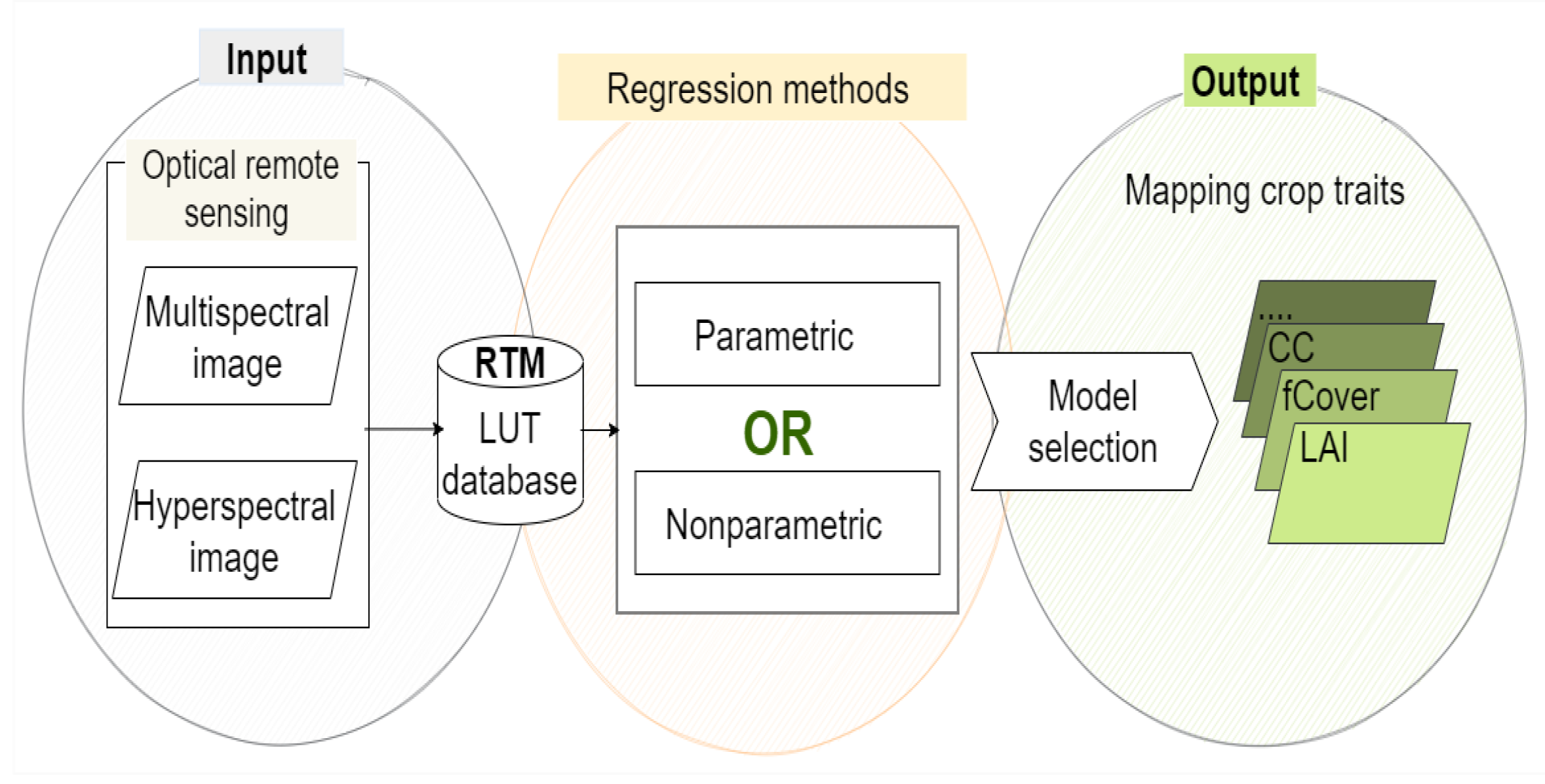
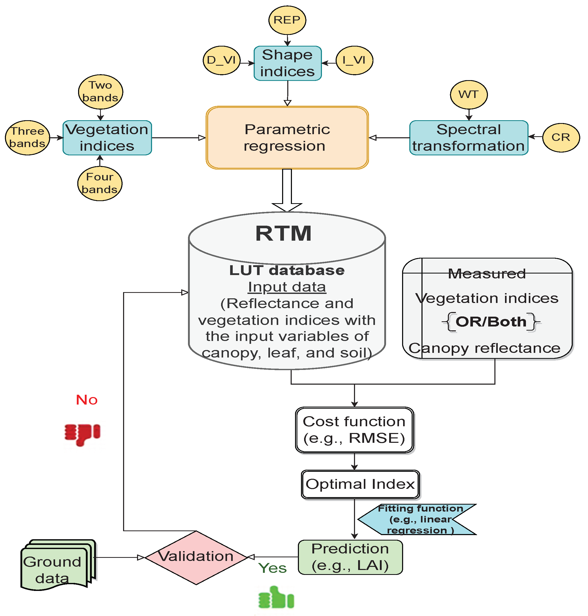

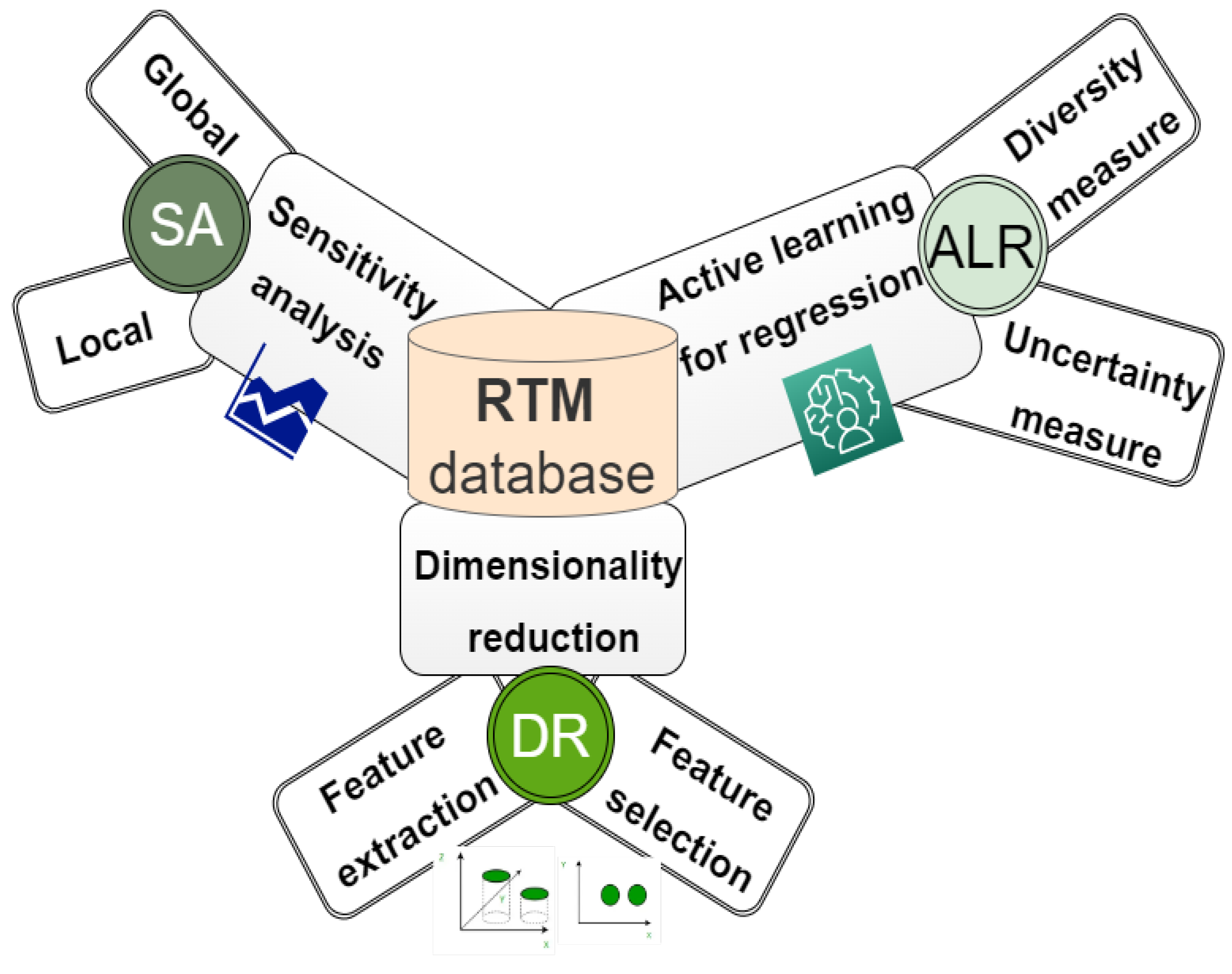
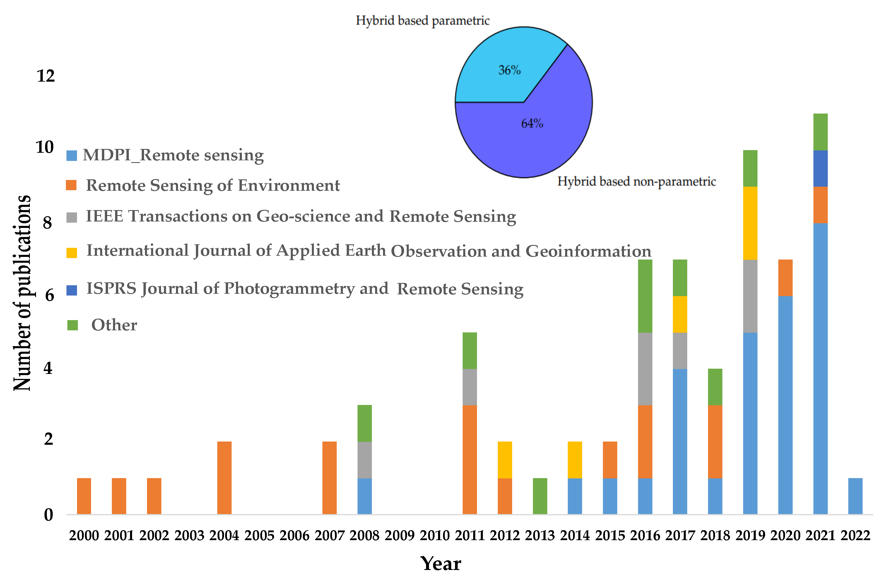
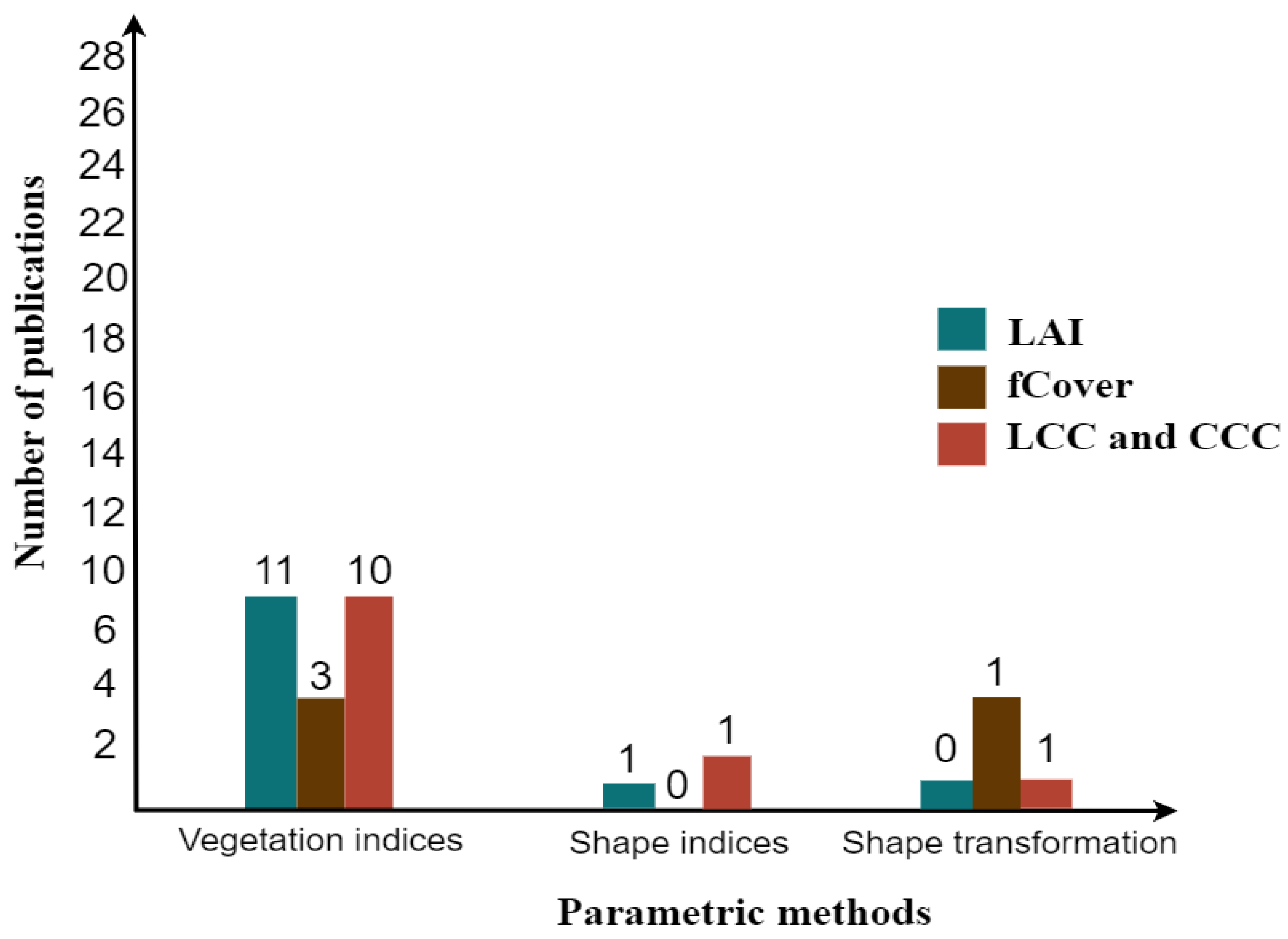
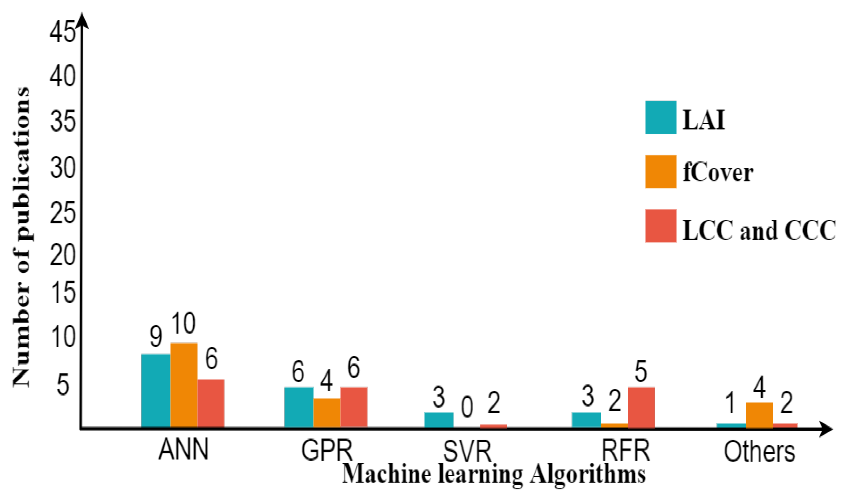
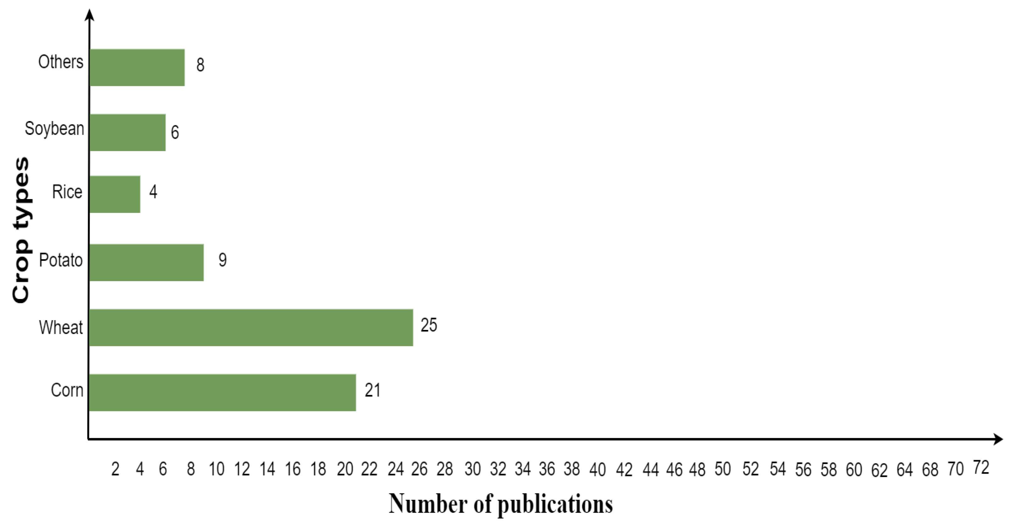
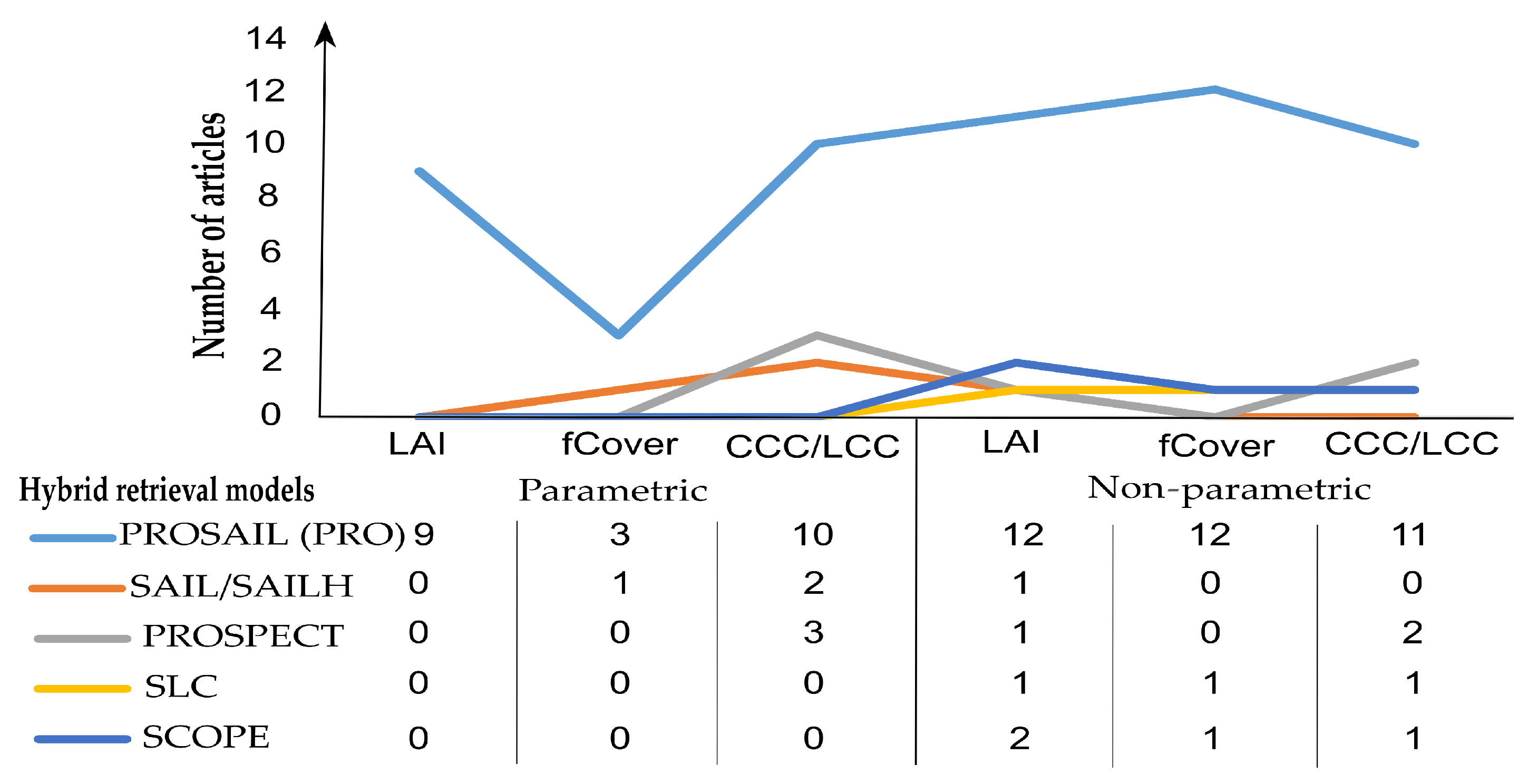

Publisher’s Note: MDPI stays neutral with regard to jurisdictional claims in published maps and institutional affiliations. |
© 2022 by the authors. Licensee MDPI, Basel, Switzerland. This article is an open access article distributed under the terms and conditions of the Creative Commons Attribution (CC BY) license (https://creativecommons.org/licenses/by/4.0/).