Abstract
LiDAR is an excellent source of elevation data used in many surveys. The spaceborne handle system, Global Ecosystem Dynamics Investigation (GEDI), provides ground elevation information with high accuracy except for areas with steep slopes. GEDI data have a lot of noise from atmospheric conditions, and therefore filtering procedures are mandatory to select the best dataset. The dataset presents uncertainties of different magnitudes, with values reaching more than 100 m of difference between the reference data and the GEDI data. The challenge is to find a criterion to determine a threshold to filter accurate GEDI samples. This research aims to identify the threshold based on the difference values between the reference data and the GEDI data to select the maximum number of samples with low RMSE values. Therefore, we used the Kolmogorov–Smirnov (KS) non-parametric test to define the best threshold based on a normal distribution. Our results demonstrated a lower RMSE value with a high number of samples when compared with the quality flag parameter threshold, even using sensitivity parameter thresholds. This method is useful for achieving the best possible accuracy from GEDI data worldwide.
1. Introduction
Advances in light detection and ranging (LiDAR) technology have produced accurate terrain altitude with airborne laser scanning (ALS). Many scientific studies use ground elevation and canopy heights in various applications such as urban environment mapping of Land Use and Land Cover (LULC) [1,2,3], extracting objects such as buildings [4], estimating urban tree canopy and heights [5,6], detecting roads [7], modeling floods and wetlands [8,9], quantifying urban landscape changes under a historical perspective [10], and investigating the Digital Elevation Model (DEM) generation process and upward fusion with another more generic DEM [11,12]. One problem is the high cost of ALS, with surveys covering small areas.
There are few experiences in the development of spaceborne LiDAR systems [13]. The first experiences started with Shuttle Laser Altimeter (SLA) [14], followed by ICESat [15]. Currently, the ICESat 2 altimeter mission [16] aims to estimate changes in polar ice-sheet volume to evaluate their impact on global sea level. Moreover, LiDAR data from space provides biomass quantification by measuring vegetation canopy heights, demonstrating its potential in forest studies.
In this way, the Global Ecosystem Dynamics Investigation (GEDI), launched in 2018, is an advanced spaceborne LiDAR system measuring the returned full waveform. The GEDI system comprises 3 lasers producing 8 tracks of data, separated by 600 m in the along-flight track direction, onboard the Japanese Experiment Module-Exposed Facility (JEM-EF) on the International Space Station (ISS). The lasers shoot fires at a frequency of 242 Hz and produce on-ground measurements over a 25 m-wide footprint. Each track’s footprint centers are separated by 60 m along-track direction, producing terrain and canopy information with an estimated accuracy of 10–20 m horizontally and about 50 cm vertically [13]. Future post-processing and pointing, ranging, and timing calibration updates improve data accuracy.
The GEDI data provide canopy heights, canopy vertical profile, Relative Heights (RH), and surface elevation. Data availability encourages the scientific community to produce several studies, such as: mapping 3D forest structure in the United States [17], forest stand volume estimation in a mixed forest area of northeast China [18], structural characterization of old-growth forests in the Ukrainian Carpathian Mountains [19], estimation of canopy heights and aboveground biomass (AGB) in Mediterranean forests [20], detection of ancient Maya buildings in a forested environment [21], slope-adaptive assessment of GEDI waveforms for AGB estimation over mountainous areas [22], and GEDI geolocation uncertainty impact to estimate tropical forest canopy height [23].
Studies also aim to calculate the terrain accuracy of the GEDI dataset compared with other reference elevation data. Spracklen and Spracklen [19] use the TanDEM-X 12 m as reference data to estimate the relative accuracy of GEDI terrain data. Otherwise, GEDI terrain information was the elevation reference to calculate the accuracy of the sub-canopy estimation from TanDEM-X 12 m using ALOS-2 PALSAR-2 InSAR Coherence [24]. Concerning measured elevations, few studies assessed the absolute accuracy of GEDI elevation data [25,26], mainly using ALS LiDAR.
GEDI is a near-infrared (IR) optical remote sensor and suffers disturbance due to cloud cover, solar illumination, system geometries, and atmospheric conditions, among others [13], producing two categories of noise: erroneous data with more than 100 m difference with reference data, and uncertainties of measurements. Most studies used the quality flag parameter provided as GEDI ancillary information to assess and remove erroneous data from distribution before their main accuracy assessment issues [18,19,20,21,24,27,28,29,30]. Other studies optimize the use of the quality flag parameter by adjusting the sensitivity beam value adopted as a complementary analytic threshold. This ancillary information establishes a signal-to-noise ratio related to the maximum canopy cover throughout the GEDI signal, enabling ground detection [17,31]. As height differences are typically not normally distributed, the accuracy estimate of the error using RMSE is often overestimated. Therefore, the data should be as close as possible to a goodness-of-fit distribution [32,33,34,35,36]. After elimination of erroneous data, the selection of the dataset closest to the normal distribution must consider the threshold value of the difference between the GEDI and LiDAR data.
Thus, this study aims to obtain the best threshold to select only GEDI data as close as possible to normal distribution to achieve low RMSE values. Therefore, we used a normality paradigm method to remove uncertainties using the Kolmogorov–Smirnov (KS) non-parametric test, based on a non-normal test trialed in a flat urban area of Federal District, Brazil.
2. Materials and Methods
2.1. Study Area
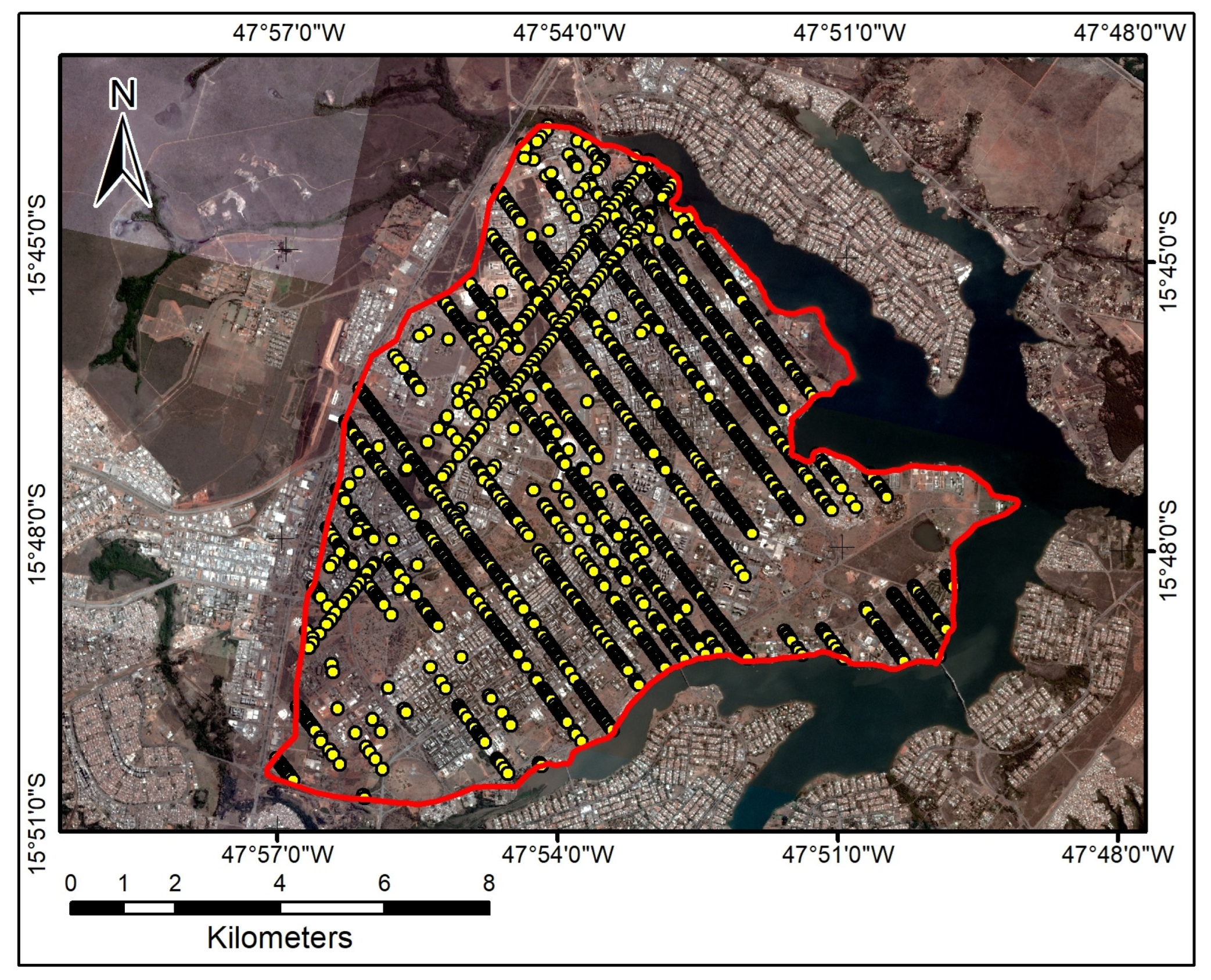
Brasília, the Federal capital of Brazil, has a population of approximately 3,000,000 inhabitants distributed in rural (3.38%) and urban (96.62%) areas [37]. Brasília’s urban environment has buildings and residences arranged in wooded areas, sparse green areas, commercial areas, and political buildings, among others. The study area is the center of Brasília and comprises the perimeter between the coordinates 47°57′19.62″W 15°43′34.62″S and 47°49′9.08″W 15°50′44.56″S (Figure 1). The relief is gentle with a mean slope of 3.07 and has ALS data available for absolute accuracy assessment. The vegetation belongs to the Cerrado biome, consisting mainly of grassland with sparse savanna and forest areas, normally located in urban conservation parks.
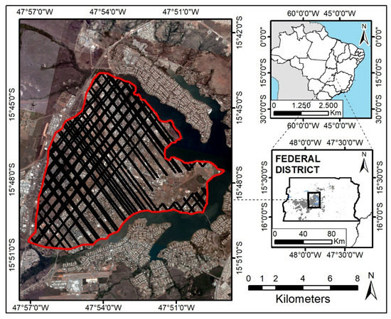
Figure 1.
Study area located in Federal District. The red line represents the center of Brasília city and the black dots are GEDI data used in this study.
2.2. GEDI Data
GEDI data is available in the Land Processes Distributed Active Archive Center (LP DAAC, https://lpdaac.usgs.gov/tools/data-pool/ (accessed on 14 April 2021)) in three products, L1B, L2A [27,38], and L2B [39] processed to guarantee the useful part of the waveform after applying smoothing to reduce noise. The L1B data product contains geolocated raw transmitted and received waveforms and ancillary information about noise and acquisition time. The L2A data product contains elevation data and height metrics of the vertical structures inside the waveform. Other data about the L2B product are vegetation metrics, such as canopy cover, vertical profile metrics, and Leaf Area Index (LAI). We processed data from the L2A considering the following information (Table 1).

Table 1.
GEDI metrics used in this study.
2.3. ALS Data
We used a digital terrain model (DTM) derived from discrete return ALS data to calculate the absolute accuracy of GEDI height estimates. The ALS data is a aero-photogrammetric product elaborated by a government campaign in the urban area, with 4 points per square meter density and 27 cm of vertical accuracy with 50 cm spatial resolution. Original ALS data has a horizontal reference system SIRGAS2000, UTM Zone 23S, ITRF2000-ellipsoid, referred vertically to MAPGEO2015.
2.4. Methods
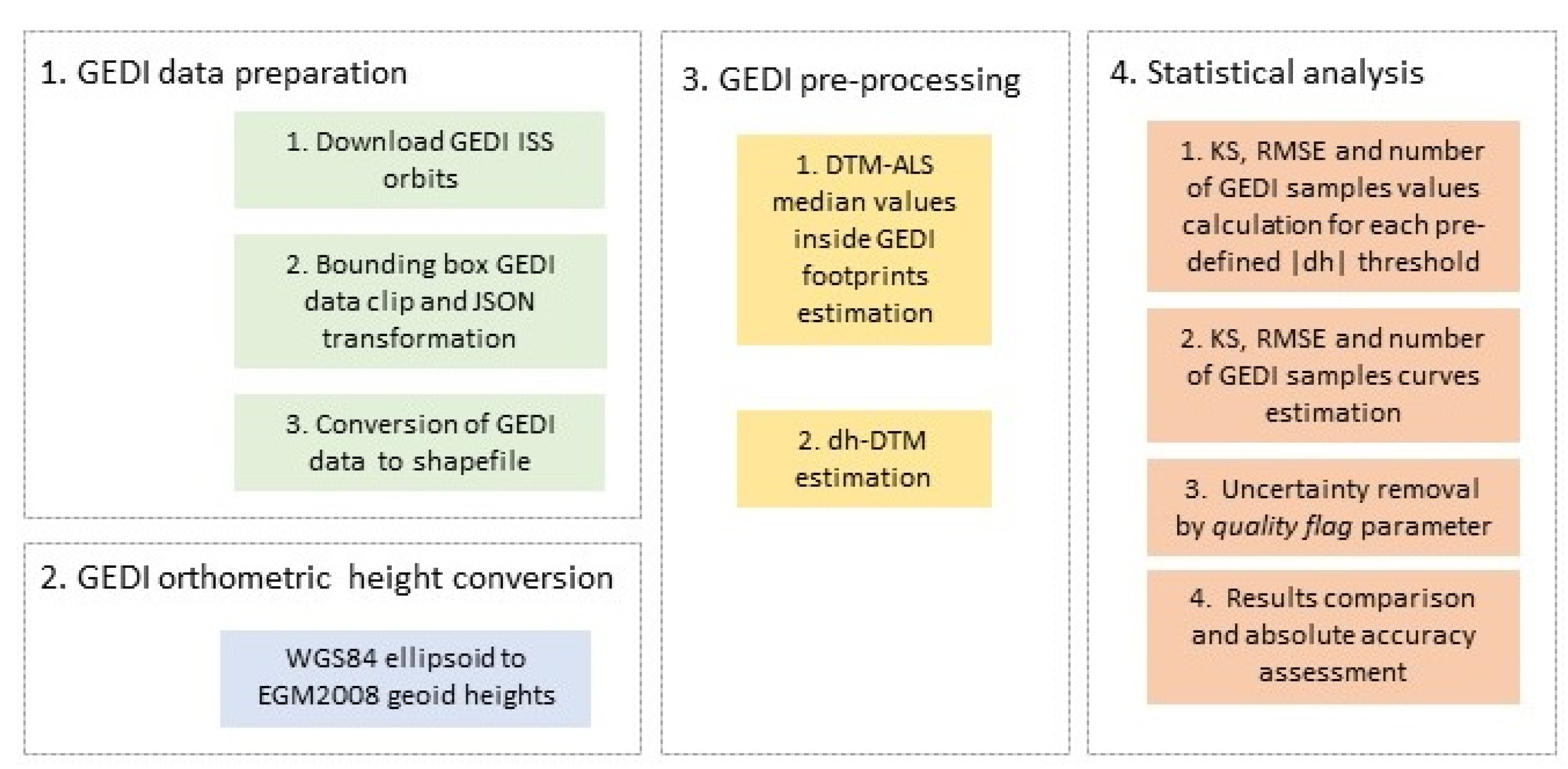
The present research has four methodological sections (Figure 2): data preparation, orthometric height transformation, pre-processing, and statistical analysis.
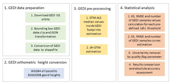
Figure 2.
Methodological flowchart.
2.4.1. GEDI Data Preparation
The GEDI Finder web service provides all available GEDI L2A products to the study area, totaling 13 orbits files within the boundary box. Table 2 lists the GEDI L2A products downloaded and the acquisition dates.
Table 2.
GEDI L2A products downloaded and acquisition dates.
We used a GEDI Subsetter python code to clip the GEDI products spatially and performed the data conversion from the GeoJSON format to shapefile using QGIS 3.16. The total number of processed footprints in the study area was 7619 between 2 June 2019 and 4 August 2020.
2.4.2. GEDI Orthometric Height Conversion
The analysis between GEDI and reference data elevations requires all height metrics to be in the same vertical reference system. The original GEDI height data are relative to the WGS 84 ellipsoid, while DTM-ALS is in the MAPGEO2015 geoid system. According to Nicacio and Dalazoana [40], the relative approach using EGM 2008 produces better results than MAPGEO2015. Thus, the conversion to orthometric heights of GEDI data used the following Equation (1):
where HEGM2008 is the derived orthometric height of GEDI data, hWGS84 is the original GEDI footprint heights referenced to the WGS84 ellipsoid, and NEGM2008 represents the EGM 2008 gravimetric geoid heights (≈ -12.5 m for study area). We used VDatum 4.2 software developed by the National Oceanic and Atmospheric Administration (NOAA) to convert the vertical datum of GEDI data, ensuring compatibility with the ALS LiDAR reference.
HEGM2008 = hWGS84 − NEGM2008
2.4.3. GEDI Pre-Processing
Each terrain height of GEDI data is a mean terrain height from the interaction between the signal and the objects within a 25 m footprint, represented by a point-shaped polygon. We extracted to every GEDI footprint attribute table the median of the intercepted cell values from DTM-ALS, regarding the difference between the spatial resolutions of both datasets. The median reduces the influence of potential uncertainties in the DTM-ALS [25].
For further statistical analysis and absolute accuracy assessment, we defined as the error the difference in height (dh) between GEDI elevation of the center of the lowest mode (ELM) value and the DTM-ALS median value (henceforth called “dh-DTM”) within each GEDI footprint.
2.4.4. Statistical Analysis
Kolmogorov–Smirnov (KS)
The statistical Kolmogorov–Smirnov (KS) non-parametric test estimates the normality in the error distribution. Applied in many remote sensing studies, the KS test, from two sets of values, compares an observed cumulative frequency distribution based on randomly collected samples and an empirical cumulative frequency distribution based on a normal distribution, expressed as and . The KS test identifies the point at which these two distributions show the maximum divergence [41], calculated through estimation of absolute divergence values D1 and D2, according to Equations (2)–(4):
The KS test has the advantage of not assuming the previous normality distribution of the samples [42], increasing the ability to explain the normality of data with larger sample sizes and matching the powerful Shapiro–Wilk (SW), Anderson–Darling (AD), and Lilliefors (LF) tests [43,44]. The KS curve estimates used the dh-DTM distribution according to two groups of pre-defined absolute thresholds. The first group admitted a 10 m interval (100, 90, 80, 70, 60, 50, 40, 30, 20, and 10 m) and the second more detailed considered a 1 m interval below the 10 m absolute dh-DTM threshold (9, 8, 7, 6, 5, 4, 3, 2, and 1 m). These interval thresholds allowed us to find the optimal point for data normality with reduced uncertainties. Assuming a similar approach, around 99.92% of samples above the first absolute threshold (<100 m) have amplitude errors from 1668.69 to 14,709.78 m, indicating coarse data error. Therefore, the statistical analysis started from this threshold for further accuracy comparison since the presence of such data errors in the distribution affects it negatively.
The performance analysis of the proposed uncertainties elimination method considered the RMSE of each pre-selected threshold and the RMSE curve (Equation (5)) [45]:
where Δhi is the difference between ith values of dh-DTM.
In addition, we also removed uncertainties from the total GEDI distribution using the quality flag indicator with 0 for further comparison and discussion.
3. Results
3.1. Proposed KS Uncertainties Removal Method and Absolute Accuracy Assessment
Table 3 lists the number of GEDI footprints, calculated KS, and RMSE from each selected threshold. Figure 3 shows comparisons between calculated KS, the number of GEDI footprints, and RMSE curves with 10 and 1 m intervals.
Table 3.
Statistics from pre-defined thresholds of absolute value of dh-DTM.

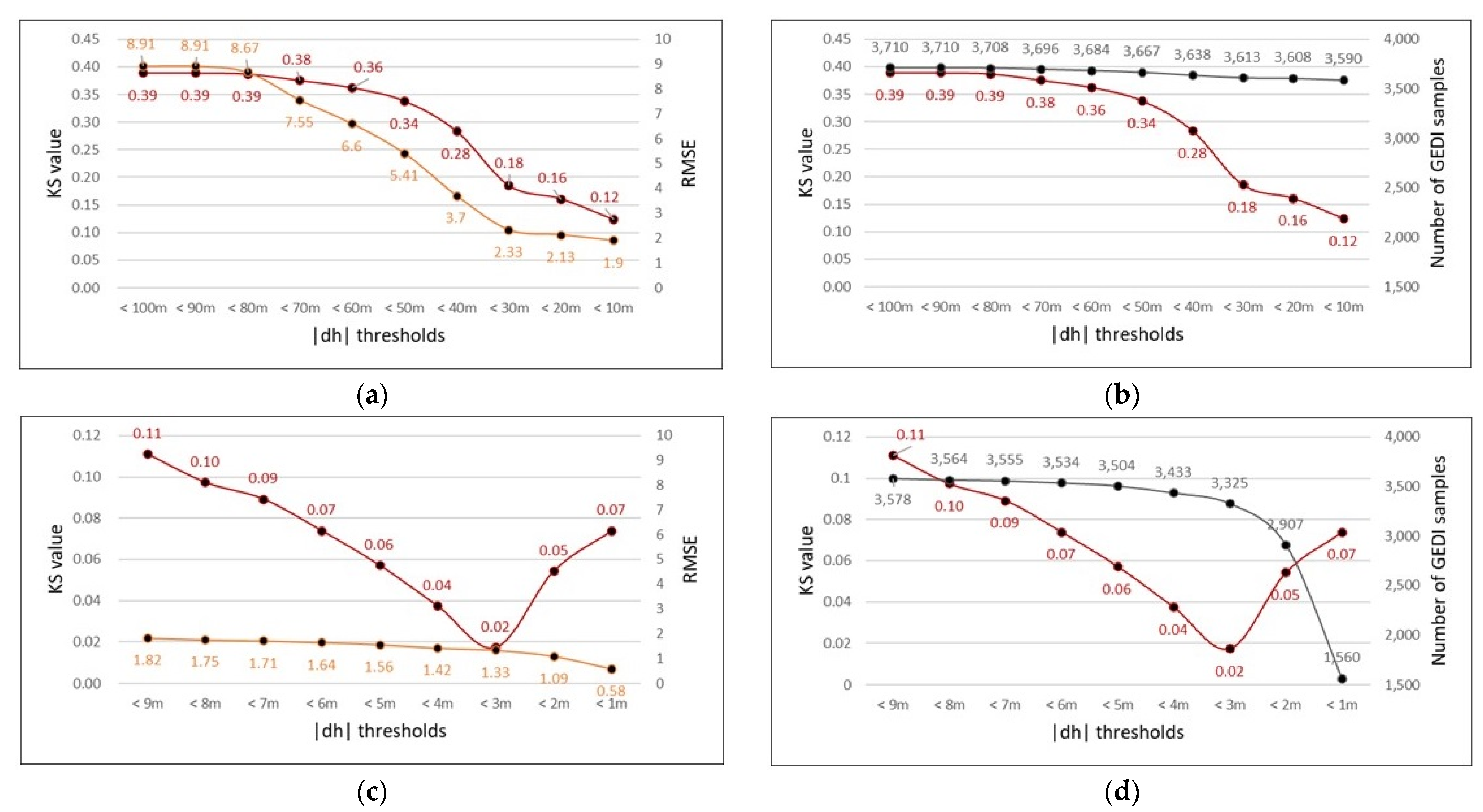
Figure 3.
Comparison between calculated KS (red color), number of GEDI samples (grey color), and RMSE (orange color) curves from absolute dh-DTM thresholds. (a) Calculated KS and RMSE values—10 m interval from |dh| < 100 m and |dh| < 10 m; (b) calculated KS value and number of GEDI samples—10 m interval from |dh| < 100 m and |dh| < 10 m; (c) calculated KS and RMSE values—1 m interval from |dh| < 9 m and |dh| < 1 m; (d) calculated KS value and number of GEDI samples —1 m interval from |dh| < 9 m and |dh| < 1 m.
Figure 3a indicates a decrease in calculated KS and RMSE values between thresholds of differences <100 and <10 m, around 68.26% and 78.67%, as expected. However, Figure 4b shows a reduction in only 120 GEDI samples, indicating few differences above 10 m absolute dh-DTM. The KS and RMSE values showed a pronounced reduction between thresholds <100 and <30 m, registering better goodness-of-fit data distribution with the removal of 97 high differences that ensured a better absolute accuracy (8.91 to 2.33 m).
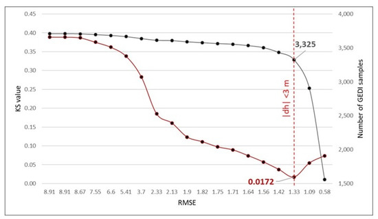
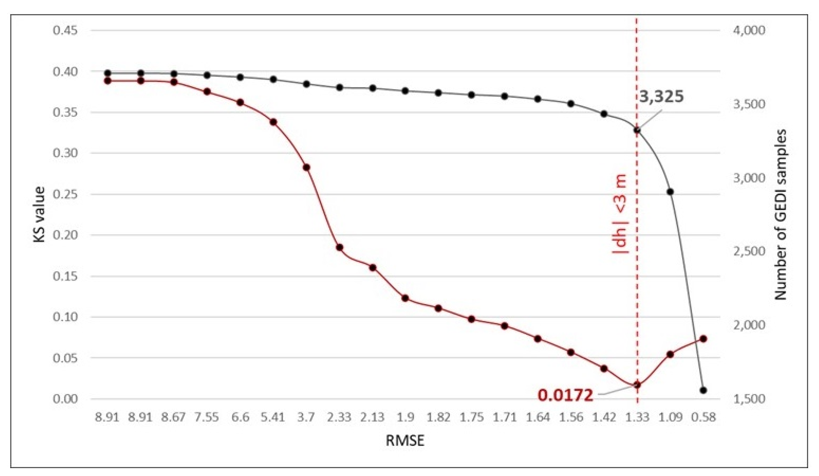
Figure 4.
Optimal threshold of calculated KS (red color), RMSE (red dashed line) values, and the number of GEDI samples (grey color).
Figure 3c,d show the KS curves, RMSE, and the number of GEDI samples in more detail, considering the 1 m interval between the <9 and <1 m absolute dh-DTM thresholds. A function inflection point occurs in <3 m absolute dh-DTM distribution, where the dispersion of data found its optimal normal fit distribution. Calculated KS decreased from 0.1109 to 0.0172 until the identified inflection point, at an approximately constant rate in each 1 m decrease in absolute dh-DTM. Moreover, there is no gain in absolute accuracy (1.82 to 1.33 m), and the number of GEDI samples decreased by 7.07% with the removal of 253 smaller differences from the distribution. However, absolute dh-DTM thresholds lower than 3 m have increased KS values, a high reduction in the number of samples, around 53.08% (3325 to 1560), and a small gain of approximately 0.75 m in absolute accuracy. Therefore, minor differences in dh-DTM do not produce a better fit to the Gaussian distribution.
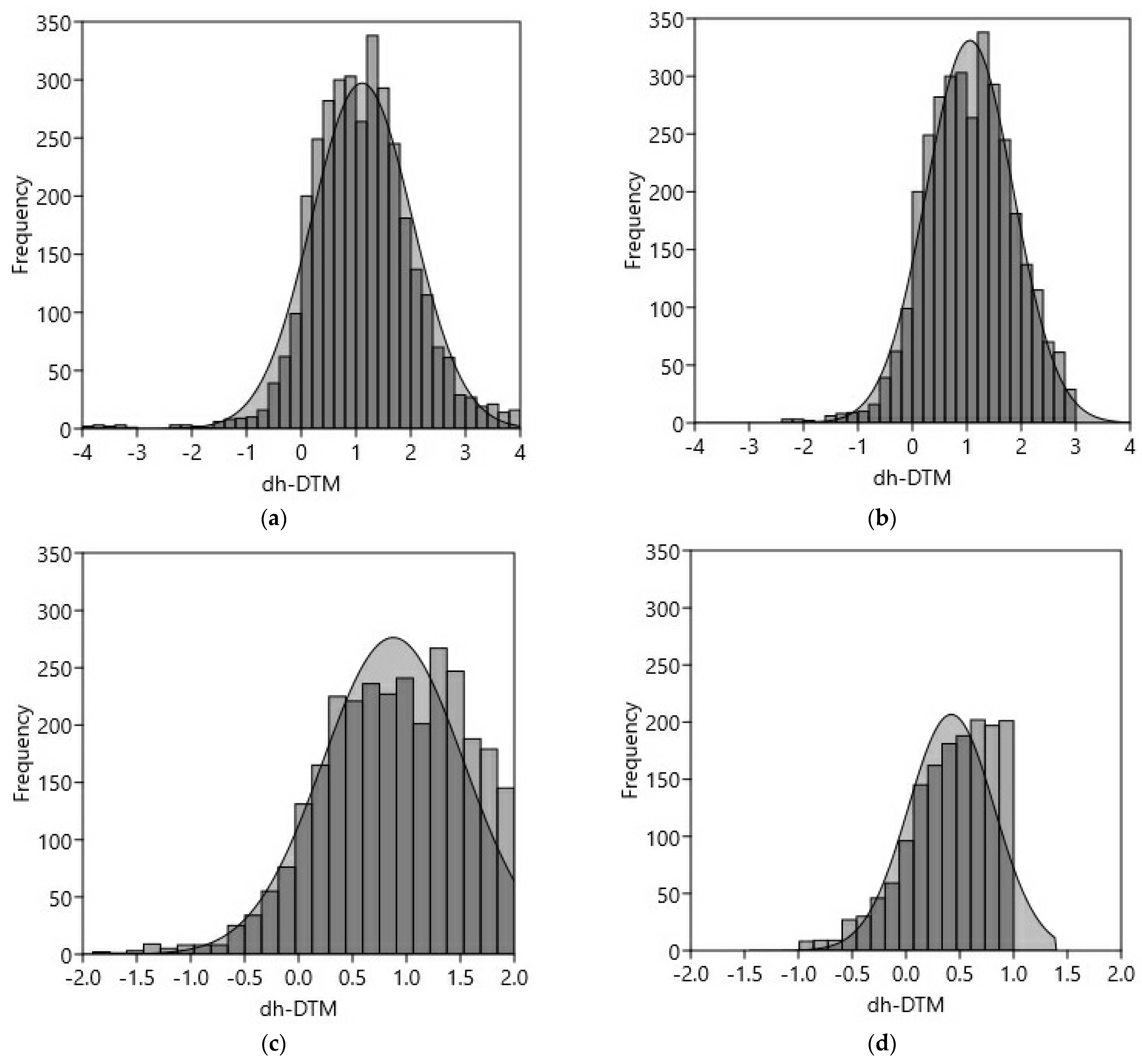
Figure 4 shows the optimal threshold considering calculated KS, RMSE values, and the number of GEDI samples. The optimal goodness-of-fit threshold converges with the best GEDI sample arrangement, reaching an RMSE value of 1.33 m. Figure 5 shows the histograms of <4, <3, <2, and <1 m absolute difference thresholds (dh-DTM). The <3 m threshold fit with the best normal distribution (Figure 5b). Below 2 m, data tends to non-normal distribution, as shown by calculated KS values.

Figure 5.
Histograms showing the dh-DTM distribution: (a) |dh| < 4 m; (b) |dh| < 3 m; (c) |dh| < 2 m; (d) |dh| < 1 m. The shaded grey curve is the normal distribution.
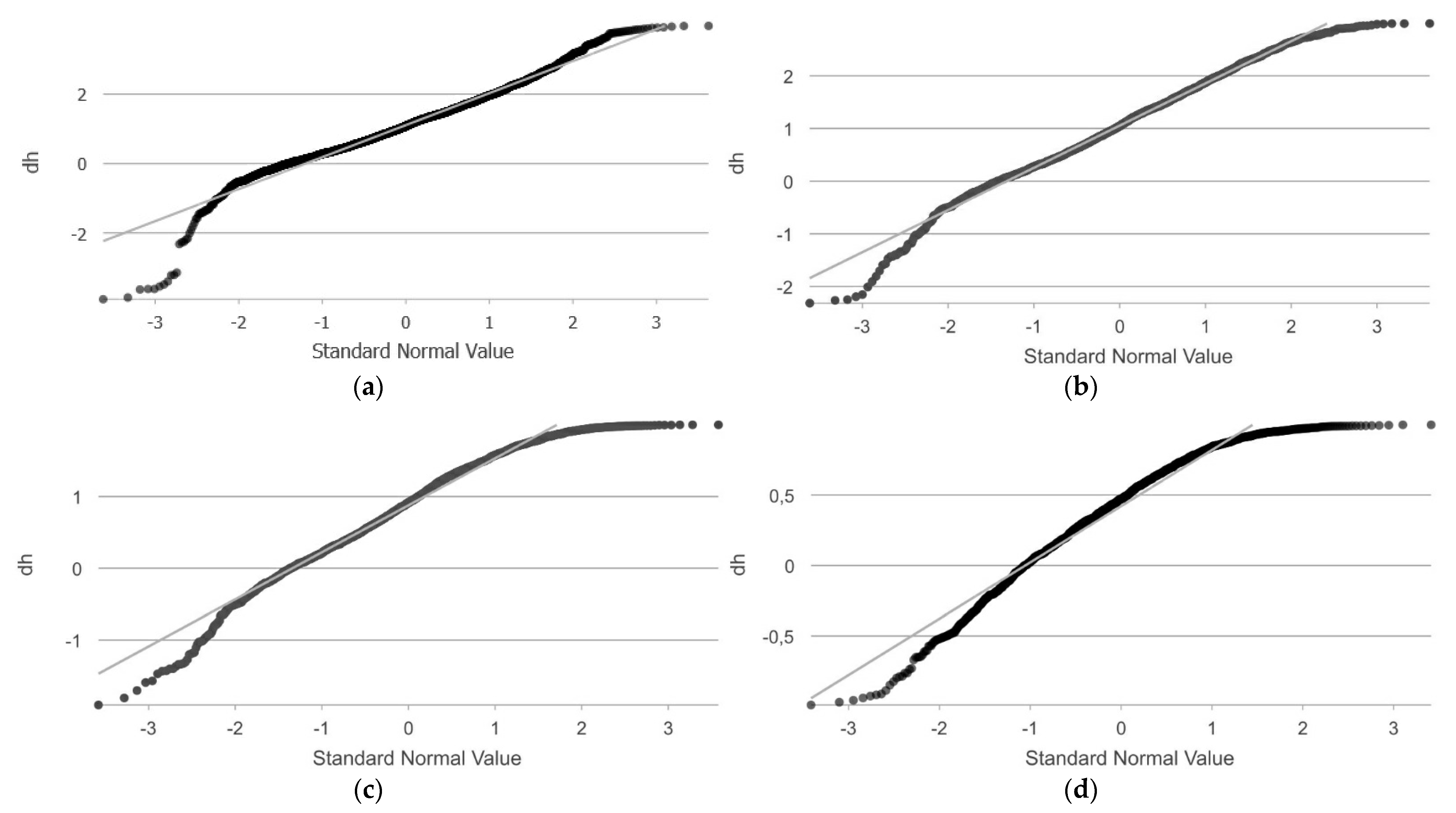
Figure 6 shows the normal quantile–quantile (QQ) plots graphical method for diagnosing differences between the probability distribution of the GEDI dataset and theoretical normal distribution. We observed a slightly sigmoid shape of the empirical distribution compared to the straight line of the normal curve. The analysis of the QQ plots reveals the improvement in goodness fit with reduction in absolute thresholds dh-DTM and the optimal normal behavior of the threshold of 3 m. Moreover, absolute dh-DTM distributions lower than 3 m show a non-normal statistical distribution.

Figure 6.
Quantile–quantile plots showing distributions of: (a) |dh| < 4 m; (b) |dh| < 3 m; (c) |dh| < 2 m; (d) |dh| < 1 m. The light grey line indicates the reference of the QQ plot.
Figure 7 and Figure 8 show the GEDI uncertainty footprints eliminated above and below the optimal dh-DTM distribution threshold identified. It is possible to observe the spatial distribution of the 385 and 1765 uncertainty samples eliminated, respectively, above the inflection point identified on the KS curve and below it. Although there is no spatial pattern in the eliminated GEDI samples, we can observe a significant loss of accurate data from the GEDI distribution.
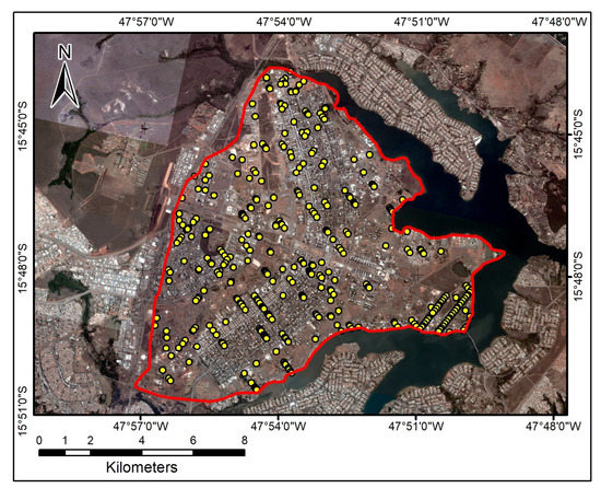
Figure 7.
Location of the GEDI samples excluded from <100 to <3 m thresholds. The yellow dots are the GEDI samples.

Figure 8.
Location of the GEDI samples excluded from <3 to <1 m threshold. The yellow dots are the GEDI samples.
3.2. Comparison with Uncertainties Removal by Quality Flag Parameter and GEDI Sensitivity Beam Data Dispersion
Table 4 lists the number of GEDI samples, KS, and RMSE values for dh-DTM distribution after removing uncertainties by quality flag and the IQR threshold approach. Figure 9 shows its respective boxplots of dh-DTM uncertainties.
Table 4.
Statistics from the dh-DTM quality flag to remove uncertainties and its IQR threshold improvement.
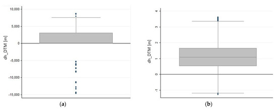
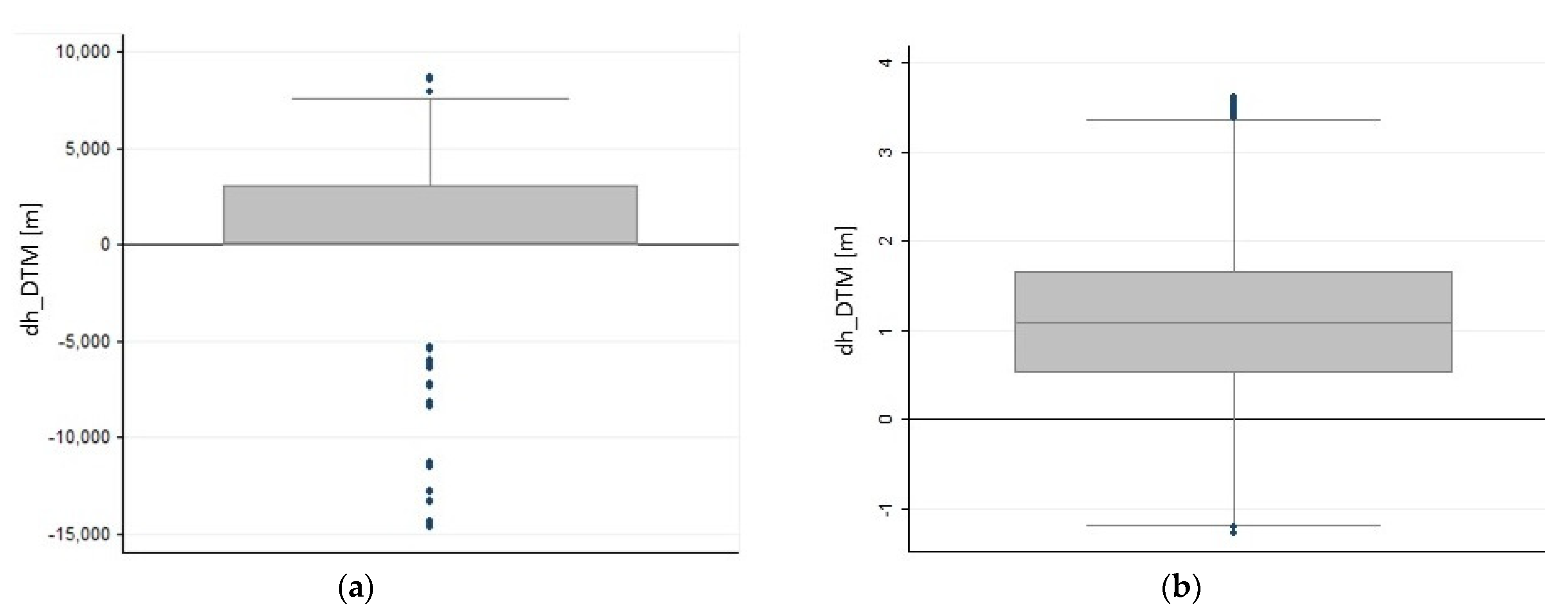
Figure 9.
Boxplots showing the distribution of dh-DTM of the total GEDI dataset. (a) Original distribution of dh-DTM; (b) resulted distribution of dh-DTM after applying a second step based on IQR thresholds.
For the total GEDI dataset (7619 samples), with the erroneous data, the absolute accuracy is 5946.73 m. Even after removing all data with quality flag value “0”, the RMSE value is 260.46 m, indicating high GEDI dh-DTM distribution errors (Table 4). Thus, we applied another step to remove remaining erroneous data using thresholds of 1.5 times the interquartile range (IQR) minus the first quartile plus third quartile, establishing a benchmark. Results indicated a better dh-DTM distribution with RMSE of 1.40 m considering 2883 GEDI footprints (Table 4). The proposed uncertainties removal method reached 1.33 m of RMSE selecting 3325 GEDI footprints. This result is 15.33% higher than the quality flag method benchmark in dh-DTM distribution with an absolute difference < 3 m.
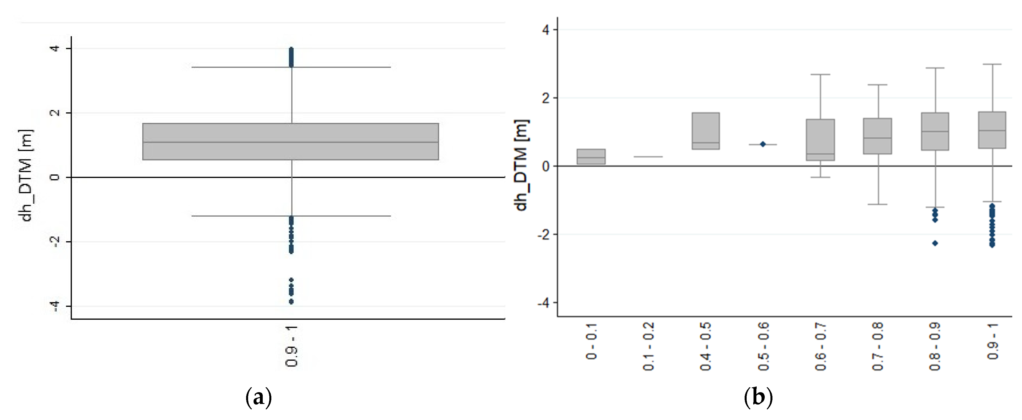
The boxplot in Figure 10a shows data selection using the 0.9 sensitivity threshold. Figure 10b shows dh-DTM <3 m in all sensitivity ranges. Those data are useful and should not be disregarded.
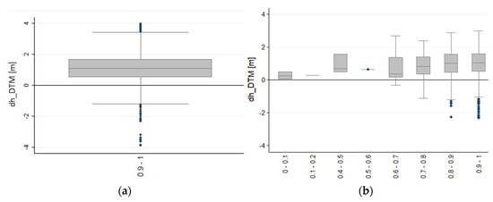
Figure 10.
Boxplots showing the distribution of dh-DTM. Data selection with 0.9 sensitivity threshold (a). Useful data along all sensitivity ranges (b).
We divided into two groups the differences between GEDI footprints derived from both uncertainty removal methods for analysis. Group 1 represents GEDI samples present in our method but not in the dataset from the quality flat removal method (with a value equal to 1). Group 2 is the opposite. Table 5 lists the number of samples and RMSE from both GEDI groups, and Figure 11 presents the spatial distribution of these GEDI groups in the study area.
Table 5.
Statistics from GEDI footprint groups.
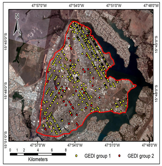
Figure 11.
Location of GEDI footprint groups derived from both uncertainty removal methods. GEDI footprints from group 1 is represented in yellow dots and group 2 in red dots.
The results indicate that 502 GEDI samples remain when applying our method to remove uncertainties, reaching an RMSE value of 1.32 m suitable for use. In contrast, the quality flag removal method keeps only 60 samples (RMSE of 3.28 m). Furthermore, the proposed method did not select the 60 GEDI samples captured by the quality flag removal method because the absolute dh-DTM is greater than 3 m. As shown in Figure 11, the increase in useful GEDI samples can assist in the DEM interpolation processes or even as reference points to support other terrain applications in the study area. These results reinforce the importance of statistical analysis of the Gaussian distribution before removing uncertainties, evidencing that the use of the quality flag parameter alone may not be sufficient to select the appropriate GEDI data. This is because the quality flag parameter disregards error distribution analysis but considers the energy, sensitivity, amplitude, and real-time surface tracking for each GEDI sample separately [27].
4. Discussion
Atmospheric conditions and system geometries influence the GEDI data and affect its quality flag measurements [13]. Thus, all related GEDI studies have an uncertainty removal approach. The challenge is to find the best threshold that can separate the signal from the noise. Articles using GEDI data determine this threshold based on the quality flag parameter. However, this procedure does not adequately consider points with low RMSE that could be used, especially in the interpolation process.
Using a quality flag threshold, Quiros et al. [28] compared GEDI data with airborne LiDAR in 10 different areas with a mean slope varying between 3.4 and 25.5 degrees and found a global RMSE of 6.05 m and 1.25 in gentle relief. Guerra-Hernández and Pascual [30] applied the quality flag parameter to remove uncertainties and reached a total of 3566 valid observations to assess height growth dynamics in fast-growing species in Spain. They found an RMSE value of 4.48 m, compatible with a higher canopy cover in their GEDI samples.
Spracklen and Spracklen [19] filtered GEDI data distribution in old-growth forests in Ukraine using the quality flag parameter. In addition, the authors had to apply a second step to remove uncertainty samples based on field data. Our study also had to apply a second step based on the IQR threshold to guarantee a useful dataset without erroneous data after quality flag filtering. Kokalj and Mast [21] used GEDI data for archaeological exploration in a forest area, considering two steps to eliminate uncertainties data: (a) visual inspection and (b) quality flag parameter followed by IQR threshold filtering. Despite obtaining an RMSE of 0.98 m, the procedure removed many GEDI samples, creating a significant data gap. Differently, our results showed similar absolute precision with a larger number of GEDI samples.
Sensitivity is ancillary GEDI information used to optimize the outlier removal data approach, where studies use a conservative threshold equal to or higher than 0.9 [17,46]. Boucher et al. [47] analyzed different sensitivity thresholds to identify ground information in various forest canopies and found that values higher than 0.95 guaranteed that 60–80% of waveforms could detect true ground heights. Our results show that it is insufficient to establish an empirical sensitivity threshold to remove GEDI uncertainties. The KS test has been widely used in remote sensing studies to verify data normality [42,48,49,50,51,52,53]. Especially in error removal, few studies used the KS test, but these have demonstrated improvements in different sensors [54,55,56,57,58]. Our approach innovates by using KS testing to analyze the error distribution and improve outlier removal, leveraging all valid GEDI data. The high sample size of the analyzed GEDI data ensures a significant performance of the adopted normality test by matching it with more robust tests, such as Shapiro-Wilk.
5. Conclusions
GEDI data are an important source of altimetry data used in several areas of knowledge. This study innovates by presenting an improved method to remove uncertainties from GEDI elevation data distribution using the KS non-parametric test and absolute accuracy assessment with a reference terrain elevation derived from ALS-DTM in an urban area with gentle relief in Federal District, Brazil. The proposed outlier removal method was better than the method using the quality flag threshold, with wide application in GEDI-related studies. Results indicate a better absolute accuracy (RMSE of 1.33) with a reduction of 56.36% (3325) of the total GEDI dataset, 15.33% higher than the sample reduction from the quality flag benchmark (2883). In addition, the quality flag procedure benchmark removed low RMSE data and selected data with RMSE that would have to be discarded. Calculating KS curves according to pre-defined absolute thresholds allows us to find the optimal inflection point where the dh-DTM distribution has a normal behavior, which occurred in <3 m. This methodology is useful for defining a threshold capable of selecting the maximum GEDI data with a low RMSE value.
This study disregards the influence of high slope and landcover on the altimetric quality of the GEDI data. Thus, future approaches in mountainous and forested areas should be conducted to determine GEDI LiDAR performance under different environmental and acquisition conditions. Furthermore, additional efforts should be conducted by adapting this methodology with other probability distribution assumptions, given that it has been demonstrated that the Laplace distribution could better represent the distribution of the terrain elevation bias [59].
Author Contributions
Conceptualization, F.L.R.B., R.F.G., O.A.d.C.J. and T.P.M.d.L.; methodology, F.L.R.B., R.F.G., O.A.d.C.J. and T.P.M.d.L.; software, F.L.R.B., R.F.G. and O.L.F.d.C.; validation, R.F.G., O.A.d.C.J. and R.A.T.G.; formal analysis, F.L.R.B., R.F.G., O.A.d.C.J. and R.A.T.G.; investigation, F.L.R.B., R.F.G., O.L.F.d.C. and T.P.M.d.L.; resources, R.F.G., O.A.d.C.J. and R.A.T.G.; data curation, F.L.R.B., R.F.G. and T.P.M.d.L.; writing—original draft preparation, F.L.R.B., R.F.G. and T.P.M.d.L.; writing—review and editing, O.A.d.C.J. and R.A.T.G.; supervision, R.F.G., O.A.d.C.J. and R.A.T.G.; project administration, F.L.R.B., R.F.G., O.A.d.C.J., R.A.T.G. and T.P.M.d.L.; funding acquisition, R.F.G., O.A.d.C.J. and R.A.T.G. All authors have read and agreed to the published version of the manuscript.
Funding
Financial support from National Council for Scientific and Technological Development—CNPq; Regulatory Agency for Water, Energy and Sewage of the Federal District—ADASA; Federal District Research Foundation—FAP/DF; and Coordination for the improvement of Higher Education Personnel (CAPES).
Acknowledgments
The authors are grateful for financial support from CNPq, ADASA, FAP/DF and CAPES fellowship (Osmar Abílio de Carvalho Júnior, Renato Fontes Guimarães and Roberto Arnaldo Trancoso Gomes). Special thanks are given to the research group of the Laboratory of Spatial Information System of the University of Brasília for technical support. The authors thank the Brazilian Ministry of Environment, who encouraged research and guaranteed all necessary support. Finally, the authors acknowledge the contribution of anonymous reviewers.
Conflicts of Interest
The authors declare no conflict of interest.
References
- Ghaseminik, F.; Aghamohammadi, H.; Azadbakht, M. Land cover mapping of urban environments using multispectral LiDAR data under data imbalance. Remote Sens. Appl. Soc. Environ. 2021, 21, 100449. [Google Scholar] [CrossRef]
- Azadbakht, M.; Fraser, C.S.; Zhang, C. Separability of targets in urban areas using features from fullwave LiDARA data. In Proceedings of the IEEE International Geoscience and Remote Sensing Symposium (IGARSS), Milan, Italy, 26–31 July 2015; pp. 5367–5370. [Google Scholar]
- Yan, W.Y.; Shaker, A.; El-Ashmawy, N. Urban land cover classification using airborne LiDAR data: A review. Remote Sens. Environ. 2015, 158, 295–310. [Google Scholar] [CrossRef]
- Awrangjeb, M.; Fraser, C.S. Automatic Segmentation of Raw LIDAR Data for Extraction of Building Roofs. Remote Sens. 2014, 6, 3716–3751. [Google Scholar] [CrossRef] [Green Version]
- Parmehr, E.G.; Amati, M.; Taylor, E.J.; Livesley, S.J. Estimation of urban tree canopy cover using random point sampling and remote sensing methods. Urban For. Urban Green. 2016, 20, 160–171. [Google Scholar] [CrossRef]
- Neto, E.M.D.C.; Rex, F.E.; Veras, H.F.P.; Moura, M.M.; Sanquetta, C.R.; Käfer, P.S.; Sanquetta, M.N.I.; Zambrano, A.M.A.; Broadbent, E.N.; Corte, A.P.D. Using high-density UAV-Lidar for deriving tree height of Araucaria Angustifolia in an Urban Atlantic Rain Forest. Urban For. Urban Green. 2021, 63, 127197. [Google Scholar] [CrossRef]
- Matkan, A.A.; Hajeb, M.; Sadeghian, S. Road Extraction from Lidar Data Using Support Vector Machine Classification. Photogramm. Eng. Remote Sens. 2014, 80, 409–422. [Google Scholar] [CrossRef] [Green Version]
- Li, B.; Hou, J.; Li, D.; Yang, D.; Han, H.; Bi, X.; Wang, X.; Hinkelmann, R.; Xia, J. Application of LiDAR UAV for High-Resolution Flood Modelling. Water Resour. Manag. 2021, 35, 1433–1447. [Google Scholar] [CrossRef]
- Mahdianpari, M.; Granger, J.E.; Mohammadimanesh, F.; Warren, S.; Puestow, T.; Salehi, B.; Brisco, B. Smart solutions for smart cities: Urban wetland mapping using very-high resolution satellite imagery and airborne LiDAR data in the City of St. John’s, NL, Canada. J. Environ. Manag. 2021, 280, 111676. [Google Scholar] [CrossRef]
- Terrone, M.; Piana, P.; Paliaga, G.; D’Orazi, M.; Faccini, F. Coupling Historical Maps and LiDAR Data to Identify Man-Made Landforms in Urban Areas. ISPRS Int. J. Geo-Inf. 2021, 10, 349. [Google Scholar] [CrossRef]
- Chen, Z.; Devereux, B.; Gao, B.; Amable, G. Upward-fusion urban DTM generating method using airborne Lidar data. ISPRS J. Photogramm. Remote Sens. 2012, 72, 121–130. [Google Scholar] [CrossRef]
- Polat, N.; Uysal, M.; Toprak, A. An investigation of DEM generation process based on LiDAR data filtering, decimation, and interpolation methods for an urban area. Measurement 2015, 75, 50–56. [Google Scholar] [CrossRef]
- Dubayah, R.; Blair, J.B.; Goetz, S.; Fatoyinbo, L.; Hansen, M.; Healey, S.; Hofton, M.; Hurtt, G.; Kellner, J.; Luthcke, S.; et al. The Global Ecosystem Dynamics Investigation: High-resolution laser ranging of the Earth’s forests and topography. Sci. Remote Sens. 2020, 1, 100002. [Google Scholar] [CrossRef]
- Garvin, J.; Bufton, J.; Blair, J.; Harding, D.; Luthcke, S.; Frawley, J.; Rowlands, D. Observations of the Earth’s topography from the Shuttle Laser Altimeter (SLA): Laser-pulse Echo-recovery measurements of terrestrial surfaces. Phys. Chem. Earth 1998, 23, 1053–1068. [Google Scholar] [CrossRef]
- Schutz, B.E.; Zwally, H.J.; Shuman, C.A.; Hancock, D.; DiMarzio, J.P. Overview of the ICESat Mission. Geophys. Res. Lett. 2005, 32, 1–4. [Google Scholar] [CrossRef] [Green Version]
- Abdalati, W.; Zwally, H.J.; Bindschadler, R.; Csatho, B.; Farrell, S.L.; Fricker, H.A.; Harding, D.; Kwok, R.; Lefsky, M.; Markus, T.; et al. The ICESat-2 Laser Altimetry Mission. Proc. IEEE 2010, 98, 735–751. [Google Scholar] [CrossRef]
- Rishmawi, K.; Huang, C.; Zhan, X. Monitoring Key Forest Structure Attributes Across the Conterminous United States by Integrating GEDI LiDAR Measurements and VIIRS Data. Remote Sens. 2021, 13, 442. [Google Scholar] [CrossRef]
- Chen, L.; Ren, C.; Zhang, B.; Wang, Z.; Liu, M.; Man, W.; Liu, J. Improved estimation of forest stand volume by the integration of GEDI LiDAR data and multi-sensor imagery in the Changbai Mountains Mixed forests Ecoregion (CMMFE), northeast China. Int. J. Appl. Earth Obs. Geoinf. 2021, 100, 102326. [Google Scholar] [CrossRef]
- Spracklen, B.; Spracklen, D. Determination of Structural Characteristics of Old-Growth Forest in Ukraine Using Spaceborne LiDAR. Remote Sens. 2021, 13, 1233. [Google Scholar] [CrossRef]
- Dorado-Roda, I.; Pascual, A.; Godinho, S.; Silva, C.; Botequim, B.; Rodríguez-Gonzálvez, P.; González-Ferreiro, E.; Guerra-Hernández, J. Assessing the Accuracy of GEDI Data for Canopy Height and Aboveground Biomass Estimates in Mediterranean Forests. Remote Sens. 2021, 13, 2279. [Google Scholar] [CrossRef]
- Kokalj, Ž.; Mast, J. Space lidar for archaeology? Reanalyzing GEDI data for detection of ancient Maya buildings. J. Archaeol. Sci. Rep. 2021, 36, 102811. [Google Scholar] [CrossRef]
- Ni, W.; Zhang, Z.; Sun, G. Assessment of Slope-Adaptive Metrics of GEDI Waveforms for Estimations of Forest Aboveground Biomass over Mountainous Areas. J. Remote Sens. 2021, 2021, 1–17. [Google Scholar] [CrossRef]
- Roy, D.P.; Kashongwe, H.B.; Armston, J. The impact of geolocation uncertainty on GEDI tropical forest canopy height estimation and change monitoring. Sci. Remote Sens. 2021, 4, 100024. [Google Scholar] [CrossRef]
- Tan, P.; Zhu, J.; Fu, H.; Wang, C.; Liu, Z.; Zhang, C. Sub-Canopy Topography Estimation from TanDEM-X DEM by Fusing ALOS-2 PARSAR-2 InSAR Coherence and GEDI Data. Sensors 2020, 20, 7304. [Google Scholar] [CrossRef]
- Adam, M.; Urbazaev, M.; Dubois, C.; Schmullius, C. Accuracy Assessment of GEDI Terrain Elevation and Canopy Height Estimates in European Temperate Forests: Influence of Environmental and Acquisition Parameters. Remote Sens. 2020, 12, 3948. [Google Scholar] [CrossRef]
- Fayad, I.; Baghdadi, N.; Bailly, J.S.; Frappart, F.; Zribi, M. Analysis of GEDI Elevation Data Accuracy for Inland Waterbodies Altimetry. Remote Sens. 2020, 12, 2714. [Google Scholar] [CrossRef]
- Hofton, M.; Blair, B.; Story, S.; Yi, D. Algorithm Theoretical Basis Document (ATBD) for GEDI Transmit and Receive Waveform Processing for L1 and L2 Products; Goddard Space Flight Center: Greenbelt, MD, USA, 2019. Available online: https://gedi.umd.edu/data/documents/ (accessed on 1 September 2019).
- Quiros, E.; Polo, M.-E.; Fragoso-Campon, L. GEDI Elevation Accuracy Assessment: A Case Study of Southwest Spain. IEEE J. Sel. Top. Appl. Earth Obs. Remote Sens. 2021, 14, 5285–5299. [Google Scholar] [CrossRef]
- Liu, A.; Cheng, X.; Chen, Z. Performance evaluation of GEDI and ICESat-2 laser altimeter data for terrain and canopy height retrievals. Remote Sens. Environ. 2021, 264, 112571. [Google Scholar] [CrossRef]
- Guerra-Hernández, J.; Pascual, A. Using GEDI lidar data and airborne laser scanning to assess height growth dynamics in fast-growing species: A showcase in Spain. For. Ecosyst. 2021, 8, 14. [Google Scholar] [CrossRef]
- Hancock, S.; Armston, J.; Hofton, M.; Sun, X.; Tang, H.; Duncanson, L.I.; Kellner, J.R.; Dubayah, R. The GEDI Simulator: A Large-Footprint Waveform Lidar Simulator for Calibration and Validation of Spaceborne Missions. Earth Space Sci. 2019, 6, 294–310. [Google Scholar] [CrossRef]
- Zandbergen, P.A. Characterizing the error distribution of lidar elevation data for North Carolina. Int. J. Remote Sens. 2011, 32, 409–430. [Google Scholar] [CrossRef]
- Oksanen, J.; Sarjakoski, T. Uncovering the statistical and spatial characteristics of fine toposcale DEM error. Int. J. Geogr. Inf. Sci. 2006, 20, 345–369. [Google Scholar] [CrossRef]
- Fisher, P. Improved Modeling of Elevation Error with Geostatistics. GeoInformatica 1998, 2, 215–233. [Google Scholar] [CrossRef]
- López-Vázquez, C. Improving the Elevation Accuracy of Digital Elevation Models: A Comparison of Some Error Detection Procedures. Trans. GIS 2000, 4, 43–64. [Google Scholar] [CrossRef]
- Bonin, O.; Rousseaux, F. Digital Terrain Model Computation from Contour Lines: How to Derive Quality Information from Artifact Analysis. GeoInformatica 2005, 9, 253–268. [Google Scholar] [CrossRef]
- Governo do Distrito Federal (GDF). Zoneamento Ecológico-Econômico do Distrito Federal (ZEE/DF): Matriz Socioeconômica; GDF: Brasília, Brazil, 2017. Available online: http://www.zee.df.gov.br/ (accessed on 1 September 2019).
- Luthcke, S.B.; Rebold, T.; Thomas, T.; Pennington, T. Algorithm Theoretical Basis Document (ATBD) for GEDI Waveform Geolocation for L1 and L2 Products; Goddard Space Center: Greenbelt, MD, USA, 2019. Available online: https://lpdaac.usgs.gov/documents/579/GEDI__WFGEO_ATBD_v1.0.pdf (accessed on 1 September 2019).
- Tang, H.; Armston, J. Algorithm Theoretical Basis Document (ATBD) for GEDI L2B Footprint Canopy Cover and Vertical Profile Metrics; Goddard Space Flight Center: Greenbelt, MD, USA, 2019. Available online: https://lpdaac.usgs.gov/documents/588/GEDI_FCCVPM_ATBD_v1.0.pdf (accessed on 1 September 2019).
- Nicácio, E.; Dalazoana, R. Comparison between absolute and relative approaches in altimetric determinations based on GNSS observations and Global Geopotencial Models. Rev. Bras. Cartogr. 2018, 70, 1–39. [Google Scholar] [CrossRef]
- Corder, G.W.; Foreman, D.I. Nonparametric Statistics for Non-Statisticians: A Step-by-Step Approach; John Wiley & Sons: Hoboken, NJ, USA, 2011; ISBN 9780470454619. [Google Scholar]
- Czajlik, Z.; Árvai, M.; Mészáros, J.; Nagy, B.; Rupnik, L.; Pásztor, L. Cropmarks in Aerial Archaeology: New Lessons from an Old Story. Remote Sens. 2021, 13, 1126. [Google Scholar] [CrossRef]
- Razali, N.M.; Wah, Y.B. Power comparisons of Shapiro-Wilk, Kolmogorov-Smirnov, Lilliefors and Anderson-Darling tests. J. Stat. Model. Anal. 2011, 2, 13–14. [Google Scholar]
- Farrell, P.J.; Rogers-Stewart, K. Comprehensive study of tests for normality and symmetry: Extending the Spiegelhalter test. J. Stat. Comput. Simul. 2006, 76, 803–816. [Google Scholar] [CrossRef]
- Gdulová, K.; Marešová, J.; Moudrý, V. Accuracy assessment of the global TanDEM-X digital elevation model in a mountain environment. Remote Sens. Environ. 2020, 241, 111724. [Google Scholar] [CrossRef]
- Potapov, P.; Li, X.; Hernandez-Serna, A.; Tyukavina, A.; Hansen, M.C.; Kommareddy, A.; Pickens, A.; Turubanova, S.; Tang, H.; Silva, C.E.; et al. Mapping global forest canopy height through integration of GEDI and Landsat data. Remote Sens. Environ. 2021, 253, 112165. [Google Scholar] [CrossRef]
- Boucher, P.; Hancock, S.; Orwig, D.; Duncanson, L.; Armston, J.; Tang, H.; Krause, K.; Cook, B.; Paynter, I.; Li, Z.; et al. Detecting Change in Forest Structure with Simulated GEDI Lidar Waveforms: A Case Study of the Hemlock Woolly Adelgid (HWA; Adelges tsugae) Infestation. Remote Sens. 2020, 12, 1304. [Google Scholar] [CrossRef] [Green Version]
- Dial, R.; Chaussé, P.; Allgeier, M.; Smeltz, T.; Golden, T.; Day, T.; Wong, R.; Andersen, H.-E. Estimating Net Primary Productivity (NPP) and Debris-Fall in Forests Using Lidar Time Series. Remote Sens. 2021, 13, 891. [Google Scholar] [CrossRef]
- Junior, J.A.S.; Pacheco, A.D.P. Avaliação de incêndio em ambiente de Caatinga a partir de imagens Landsat-8, índice de vegetação realçado e análise por componentes principais. Ciência Florest. 2021, 31, 417–439. [Google Scholar] [CrossRef]
- Wang, T.; Yu, P.; Wu, Z.; Lu, W.; Liu, X.; Li, Q.P.; Huang, B. Revisiting the Intraseasonal Variability of Chlorophyll-a in the Adjacent Luzon Strait with a New Gap-Filled Remote Sensing Data Set. IEEE Trans. Geosci. Remote Sens. 2021, 60, 4201311. [Google Scholar] [CrossRef]
- Contador, T.M.; Alcântara, E.; Rodrigues, T.; Park, E. Remote sensing of water transparency variability in the Ibitinga reservoir during COVID-19 lockdown. Remote Sens. Appl. Soc. Environ. 2021, 22, 100511. [Google Scholar] [CrossRef]
- Luiz, A.J.B.; de Lima, M.A. Application of the kolmogorov-smirnov test to compare greenhouse gas emissions over time. Rev. Bras. Biom. 2021, 39, 60–70. [Google Scholar] [CrossRef]
- Tariq, A.; Shu, H.; Kuriqi, A.; Siddiqui, S.; Gagnon, A.; Lu, L.; Linh, N.T.T.; Pham, Q.B. Characterization of the 2014 Indus River Flood Using Hydraulic Simulations and Satellite Images. Remote Sens. 2021, 13, 2053. [Google Scholar] [CrossRef]
- Baier, G.; He, W.; Yokoya, N. Robust Nonlocal Low-Rank SAR Time Series Despeckling Considering Speckle Correlation by Total Variation Regularization. IEEE Trans. Geosci. Remote Sens. 2020, 58, 7942–7954. [Google Scholar] [CrossRef]
- Broadwater, J.B.; Chellappa, R. Adaptive Threshold Estimation via Extreme Value Theory. IEEE Trans. Signal Process. 2010, 58, 490–500. [Google Scholar] [CrossRef]
- Lakshmanan, V.; Debrunner, V.; Rabin, R. Texture-based segmentation of satellite weather imagery. IEEE Int. Conf. Image Process. 2000, 2, 732–735. [Google Scholar] [CrossRef] [Green Version]
- Aguilar, F.J.; Mills, J.P. Accuracy assessment of lidar-derived digital elevation models. Photogramm. Rec. 2008, 23, 148–169. [Google Scholar] [CrossRef]
- Giménez, M.G.; de Jong, R.; Della Peruta, R.; Keller, A.; Schaepman, M.E. Determination of grassland use intensity based on multi-temporal remote sensing data and ecological indicators. Remote Sens. Environ. 2017, 198, 126–139. [Google Scholar] [CrossRef]
- Becek, K. Investigation of elevation bias of the SRTM-C and X-band digital elevation models. Int. Arch. Photogramm. Remote Sens. Spat. Inf. Sci. 2008, 37, 105–110. [Google Scholar]


Publisher’s Note: MDPI stays neutral with regard to jurisdictional claims in published maps and institutional affiliations. |
© 2022 by the authors. Licensee MDPI, Basel, Switzerland. This article is an open access article distributed under the terms and conditions of the Creative Commons Attribution (CC BY) license (https://creativecommons.org/licenses/by/4.0/).