Article

Long-Distance Multi-Vehicle Detection at Night Based on Gm-APD Lidar

National Key Laboratory of Science and Technology on Tunable Laser, Institute of Opto-Electronic, Harbin Institute of Technology, Harbin 150001, China
*
Author to whom correspondence should be addressed.
Remote Sens. 2022, 14(15), 3553; https://doi.org/10.3390/rs14153553
Submission received: 20 June 2022 / Revised: 21 July 2022 / Accepted: 21 July 2022 / Published: 24 July 2022

Abstract

:
Long-distance multi-vehicle detection at night is critical in military operations. Due to insufficient light at night, the visual features of vehicles are difficult to distinguish, and many missed detections occur. This paper proposes a two-level detection method for long-distance nighttime multi-vehicles based on Gm-APD lidar intensity images and point cloud data. The method is divided into two levels. The first level is 2D detection, which enhances the local contrast of the intensity image and improves the brightness of weak and small objects. With the confidence threshold set, the detection result greater than the threshold is reserved as a reliable object, and the detection result less than the threshold is a suspicious object. In the second level of 3D recognition, the suspicious object area from the first level is converted into the corresponding point cloud classification judgment, and the object detection score is obtained through comprehensive judgment. Finally, the object results of the two-level recognition are merged into the final detection result. Experimental results show that the method achieves a detection accuracy of 96.38% and can effectively improve the detection accuracy of multiple vehicles at night, which is better than the current state-of-the-art detection methods.

1. Introduction

In future information-based warfare, improving the situational awareness of the battlefield can effectively improve the overall control of the war. All major military powers are strengthening the development and research of related technologies. The detection and recognition of military objects is the key technology that affects battlefield situational awareness [1,2,3]. The environment where military objects are located is more complex. Plains, forests, and valleys may be their hiding places, and multiple objects can appear simultaneously. Therefore, it is of great significance to carry out research on the detection technology of multi-military objects on the battlefield in complex environments. Among them, the detection of long-distance objects at night has specific challenges due to insufficient lighting at night and small objects. Vehicles are critical objects in military operations, and it is of great significance to detect long-distance, weak, and small vehicle objects at night.
As a virtual image acquisition device, the camera has the characteristics of high resolution, strong semantics, and simple data processing. It can provide more texture detail information, color perception, and classification capabilities. However, it has limited ability in distance estimation, is easily affected by ambient light, cannot provide adequate information in low light and dark environments, and cannot effectively image vehicles at night.
Infrared sensors are also widely used imaging devices. Any object with a temperature higher than absolute zero emits infrared rays. The wavelength and intensity of infrared rays emitted at different temperatures are different, which can better reflect the properties of objects. It can work in weak light and dark environments, but the image signal-to-noise ratio is low and the edge is fuzzy, so it cannot distinguish occluded objects.
As one of the essential means of object detection, lidar has been widely used in military operations [4,5,6] and civilian applications [7,8,9,10]. Lidar can work all day and is not affected by the change of the gray illumination level in the two-dimensional image. In recent years, single-photon lidar has been developed rapidly. This type of lidar has the advantages of fast detection speed, high sensitivity, strong anti-interference ability, small size, easy integration, long detection distance, and single-photon detection capability. Among them, the Geiger-mode avalanche photodiode (Gm-APD) is a new type of detector [11,12]. The Gm-APD is a single-photon detection device working in Geiger mode, which has single-photon sensitivity and picosecond time resolution. Therefore, it can be used for long-distance detection and is widely used in military operations. Gm-APD lidar can obtain the three-dimensional distance information of the object by the time-of-flight method through the time difference of laser light transmission and reception, and the relative two-dimensional intensity information of the object can be obtained by the amplitude of the echo data. It provides a reliable data source for multi-vehicle detection at night.
Lidar can acquire data in two dimensions, as shown in Figure 1. Figure 1a is the intensity image. It can be seen that although the two-dimensional image has noticeable gradient changes visually, there is no spatial structure, and the occluded object cannot be distinguished only by the intensity image. Figure 1b is the point cloud data corresponding to the intensity image of Figure 1a. Although it lacks the texture and gradient information of the intensity image, it contains the three-dimensional position information of the object in space and can better distinguish occluded objects in terms of spatial structure.
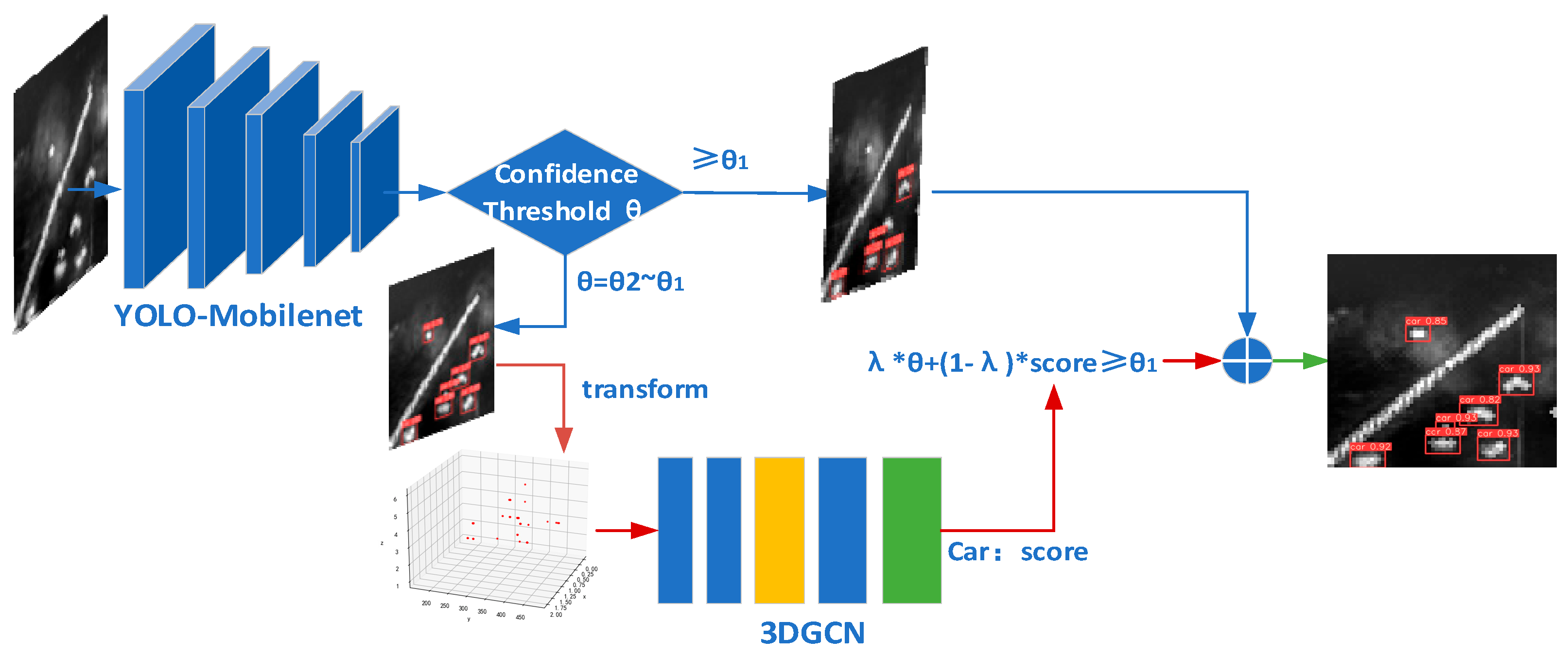
Therefore, we propose a two-level detection model based on Gm-APD lidar which uses the two-dimensional and three-dimensional information of lidar at the same time. Due to the differences in the data structures of 2D images and 3D point clouds, different network structures are used for the two forms of data. The data acquisition device is a 64 × 64 area array Gm-APD lidar. The long-distance vehicle has fewer pixels on the intensity image, and the corresponding point cloud data has fewer data points. Therefore, eight-times interpolation is performed on the intensity image and point cloud data, and the local contrast enhancement method is used for weak objects with different distances from the intensity image. The network is divided into two levels. In the first level, the YOLO network is used to detect the two-dimensional intensity image, and two confidence thresholds are set: a high threshold θ 1 and low threshold θ 2 . The detection result is greater than the first-level detection result, and the object whose confidence in the detection result is between θ 1 and θ 2 is set as the suspicious area. Next, the point cloud data are extracted in the object box of the region, the point cloud classification network is trained to obtain the classification score of the object, and the weight is set to comprehensively consider the two detection results as the output of the second level. Finally, the detection results of the two-level network are combined to obtain the final detection result.
The main contributions of the paper can be summarized as follows:
  • To solve the problem of dim and small objects not being detected at a long distance, the method of local contrast enhancement is adopted to effectively improve the brightness information of weak and small objects, which can improve the accuracy of object detection;
  • We propose a two-level detection network, which combines the two-dimensional intensity information and three-dimensional range information of lidar, effectively reducing the missed detection rate and improving the detection accuracy;
  • We propose an improved first-level object detection network. The backbone network introduces the lightweight neural network of MobilNetv3, which solves the problem of increasing the computational complexity of two-level networks without reducing the detection accuracy of the network.

2. Related Work

In recent years, with the rapid development of various imaging devices, there has been more research on vehicle detection at night. Pin Wang et al. [13] used a particle filter algorithm to introduce nonlinear statistics for vehicle detection at night. Fuzzy theory was introduced into video classification after the particle filter algorithm. Through this method, object recognition was realized, and the goal of identifying the objects of night vehicles was achieved. With the rapid development of computer vision and artificial intelligence technologies, object detection algorithms based on deep learning have been extensively studied [14,15,16]. These algorithms can automatically extract features through deep learning. More and more researchers are applying deep learning methods to the detection of vehicles at night. Danyang Huang et al. [17] proposed a depth network scheme, introduced a corner location algorithm based on Bayesian methods, and used lamp pixels to obtain more accurate corners and optical information with good generalization to assist in night vehicle detection. Experimental results showed that the method achieved 97.2% and 96.86% accuracy on the night vehicle detection dataset.
At present, vehicle detection is mainly based on visual images. The visual images at night are not clear, and the details of vehicles are not clear. Most existing nighttime vehicle detection techniques rely on paired-vehicle taillights or headlights [18,19,20]. However, when multiple vehicles appear at the same time it is impossible to accurately match the headlights, which leads to a large number of false detections, and in a dim environment weak vehicle details cannot be presented in the visual image. Therefore, some researchers use thermal infrared cameras to collect vehicle data at night. Thermal infrared cameras use the thermal radiation characteristics of objects to preserve the details of weak objects at night through thermal imaging. Shixiao Li et al. [21] proposed a car headlamp recognition method based on thermal imager data acquisition. The results showed that the accuracy of the method was 94.2%, and the recall rate was 78.7%. Although using thermal infrared images to detect objects at night can improve the detection accuracy, the infrared thermal imager only uses the two-dimensional plane information of the object. It cannot distinguish and detect occluded objects well.
Lidar has recently received more attention as a device that actively obtains three-dimensional information about an object. Therefore, more and more researchers are using lidar and other sensors to detect vehicles. Yingfeng Cai et al. [22] proposed an application of lidar and camera sensor fusion technology in vehicle detection to ensure high detection accuracy. The network structure fully uses the depth information of a lidar point cloud and RGB image for object detection. Heng Wang et al. [23] proposed a new clustering algorithm to obtain candidate vehicles from point cloud data collected by preprocessed LiDAR. A classifier trained by a support vector machine (SVM) algorithm was used to detect vehicles from candidate vehicles. The authors in [24] proposed a variant of the generalized learning system (BLS) with a unified spatial autoencoder (USAE) as a lightweight model for recognizing 3D objects. The results showed that the average recognition accuracy of the model for vehicles as well as other objects was similar to the current state-of-the-art 3D object recognition models.
The above lidar detection method data are mainly used to fuse with other sensors, which require data registration. The operation is complex and may cause specific errors. Moreover, the equipment used is based on scanning lidar data. This kind of lidar is characterized by high resolution, good concealment, and a detection range of about 100m [25,26]. However, in military operations, it is necessary to strike long-distance objects precisely, and the detection distance of 100m is far from enough. In contrast, the Gm-APD used in this study has better long-distance detection capabilities, and the method proposed in this paper only uses lidar data sources to obtain different types of data and uses its different features to detect objects, which it has more of than others. The method of sensor data fusion has better robustness.

3. Method

We used Gm-APD lidar to collect information on long-distance vehicles at night and obtain intensity images and point cloud data through advanced reconstruction algorithms [27]. Due to the characteristics of the imaging principle, there is also echo information in the background, resulting in excessive background noise in the point cloud data. It is not easy to directly use this data for object detection. The lights of vehicles at night have obvious reflectance information in the intensity image. However, the echo of the long-distance object is weak, and the image intensity value is close to the background. Therefore, a two-level object detection network was proposed for the data characteristics of our Gm-APD lidar. The contrast enhancement algorithm was used to process the weak long-distance objects in the intensity image and 2D object detection was performed on the processed intensity image as the leading judgment of the first-level network. Setting thresholds to screen out suspicious object areas and using the 3D information features of the corresponding point cloud data to make secondary judgments through the classification network can further improve the detection performance.

3.1. Data

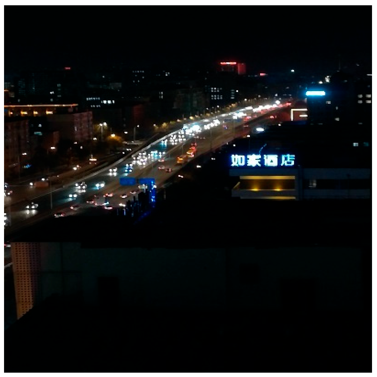
The data used in this study was obtained through a Gm-APD lidar fixed position, and the dynamic vehicle data from a 330 m to 600 m distance on the road was collected at night. The data acquisition scenario is shown in Figure 2.
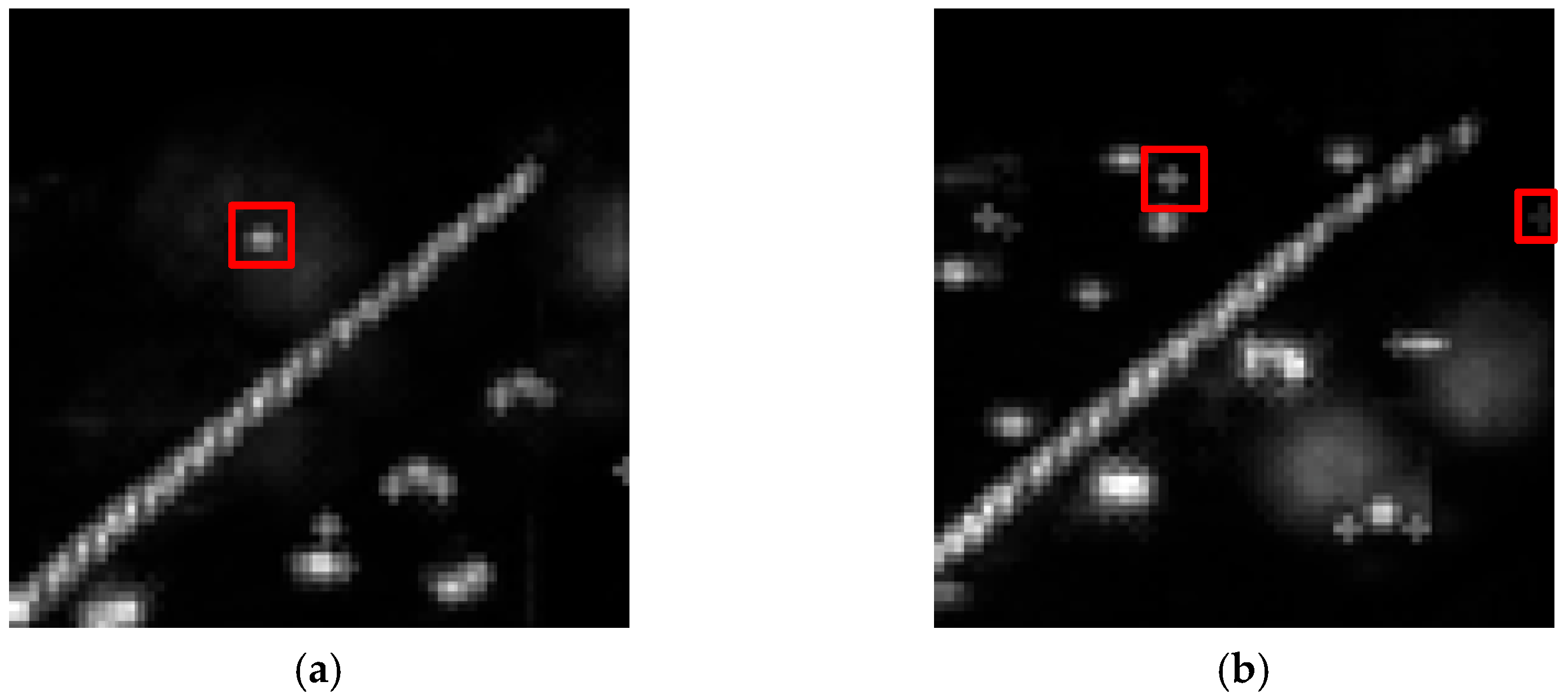
The details of the data are shown in Table 1. The specific collection time was from 20:37:19 to 21:23:50 at night. Twelve sets of data, a total of 6000 images, constituted the night vehicle dataset of this study. It can be seen from the table that the data were primarily dense objects, and some objects occupied a tiny pixel ratio in the image. The small object data in the dataset are shown in Figure 3.

3.2. Adaptive Contrast Enhancement (ACE) Algorithm

The Gm-APD lidar intensity is like an image generated by the intensity of the echoes emitted by the laser irradiating the object and then returning to the detector area array. The intensity image f ( x , y ) can be expressed as:
f ( x , y ) = H ( x , y ) + L ( x , y )
where L ( x , y ) is the low-frequency part, which is obtained by low-pass filtering of the image. H ( x , y ) is the high-frequency part, which is obtained by subtracting the low frequency part from the original image.
In this study, the detection of multiple vehicle objects at long distances was carried out. When the distance is long, and the emitted laser is interfered with by environmental factors such as atmospheric scattering in the air, the echo of the object is weak, and the generated intensity image has low contrast and is similar to the background. The ACE algorithm is different from other global image enhancement methods. This method uses local standard deviation to achieve better image local contrast enhancement than the global image enhancement method. Therefore, we used this method to enhance the intensity image. First, we enhanced the high-frequency part of the intensity image that represents the details of the medium- and long-distance weak vehicle object, multiplied the high-frequency part by a specific gain value, and then recombined it to obtain the enhanced image. Let the pixels in the image be represented as x ( i , j ) ; then, in the area with ( i , j ) as the center and the window size of ( 2 n + 1 ) ( 2 n + 1 ) , its local mean and variance can be expressed as:
m x = 1 ( 2 n + 1 ) 2 k = i n i + n l = j n j + n x ( k , l )
σ 2 x ( i , j ) = 1 ( 2 n + 1 ) 2 k = i n i + n l = j n j + n [ x ( k , l ) m x ( i , j ) ] 2
The image intensity of each point is transformed based on local region statistics. That is, the local mean m x ( i , j ) and local standard deviation σ x 2 ( i , j ) are calculated on the local region around the point. The transformed strength is:
f ( i , j ) = m x ( i , j ) + G ( i , j ) [ x ( i , j ) m x ( i , j ) ]
where the local gain G ( i , j ) is expressed as:
G ( i , j ) = α m σ i j , 0 < α < 1
where m is the global average of the image.
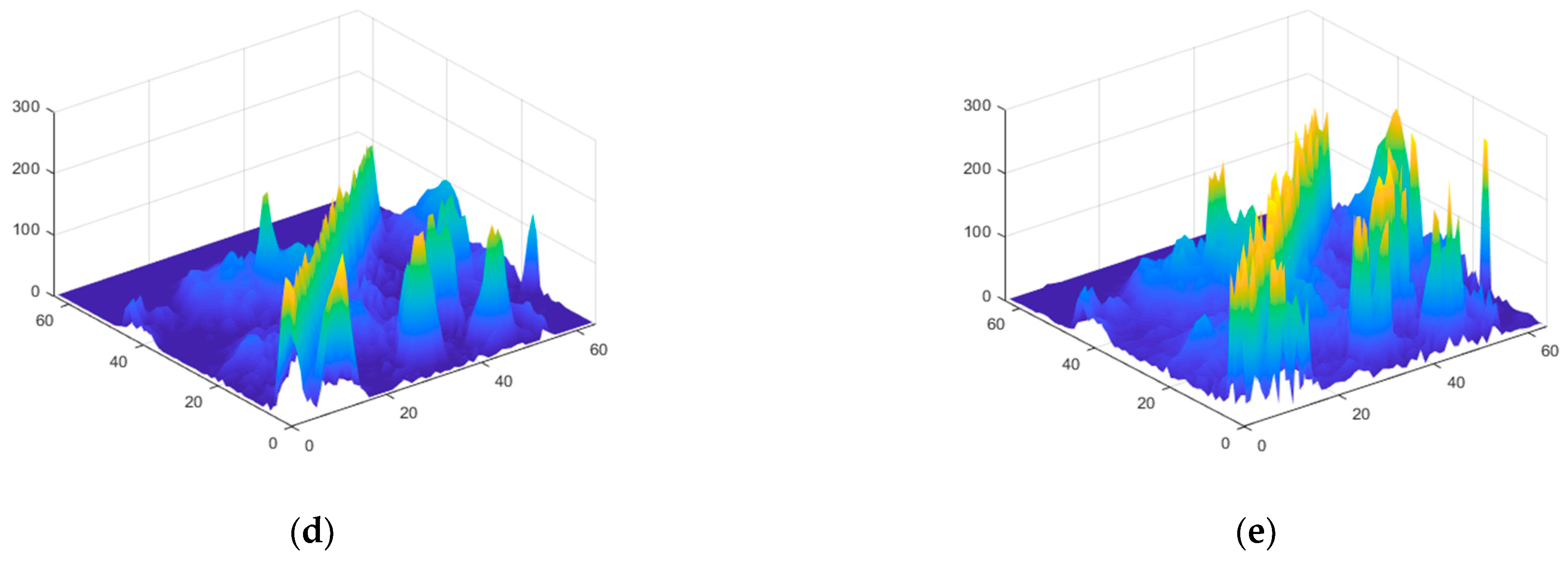
In this study, the ACE method was used to enhance the intensity image of Gm-APD, and the 3D visualization of the enhanced image was compared with the other two image enhancement algorithms, as shown in Figure 4. Figure 4a is the original two-dimensional intensity image. Figure 4b is the 3D visualization of the original 2D intensity image. Figure 4c is the 3D visualization result of the enhanced image using the ACE method. Figure 4d is a 3D visualization of the enhanced image using the contrast-limited adaptive histogram equalization (CLAHE) method. Figure 4e is a 3D visualization of the enhanced image using a linear transformation method. It can be seen from the figure that the CLAHE method cannot effectively enhance the object. Although the linear variation method enhances the object, the background is also enhanced. The ACE method used in this study cannot only effectively enhance the object, but also adjust the local gain for the background area, which is less enhanced than the intensity value of the object.
The commonly used evaluation indicators for image enhancement algorithms are peak signal-to-noise ratio, entropy, and gradient.
Peak signal-to-noise ratio (PSNR): It is an objective evaluation index of images, which is based on the error between corresponding pixels; that is, based on error-sensitive image quality evaluation [28]. The larger the PSNR value, the less the distortion. The calculation formula is:
P S N R = 20 l o g 10 ( M A X I R M S E )
where MAX I represents the maximum value of the gray level of the image point, RMSE is the root-mean-square error of the image, and the calculation formula is:
R M S E = 1 M N i = 1 M j = 1 N [ g ( i , j ) f ( i , j ) ] 2
where g ( i , j ) is the pixel value of the original image, f ( i , j ) is the pixel value of the processed image, M is the row of the image, and N is the column of the image.
Entropy: Expressed as the maximum amount of information in an image [29]. Generally speaking, an image with a large entropy value contains rich details, and the calculation formula is:
E = i p ( i ) l o g p ( i )
where p ( i ) is the probability that the pixel has brightness i.
Gradient: Measures the sharpness of the object edge. The higher the sharpness value, the higher the image clarity.
G ( x , y ) = d x ( i , j ) + d y ( i , j )
d x ( i , j ) = f ( i + 1 , j ) f ( i , j )
d y ( i , j ) = f ( i , j + 1 ) f ( i , j )
where f ( i , j ) is the image pixel value, and ( i , j ) is the coordinate of the pixel.
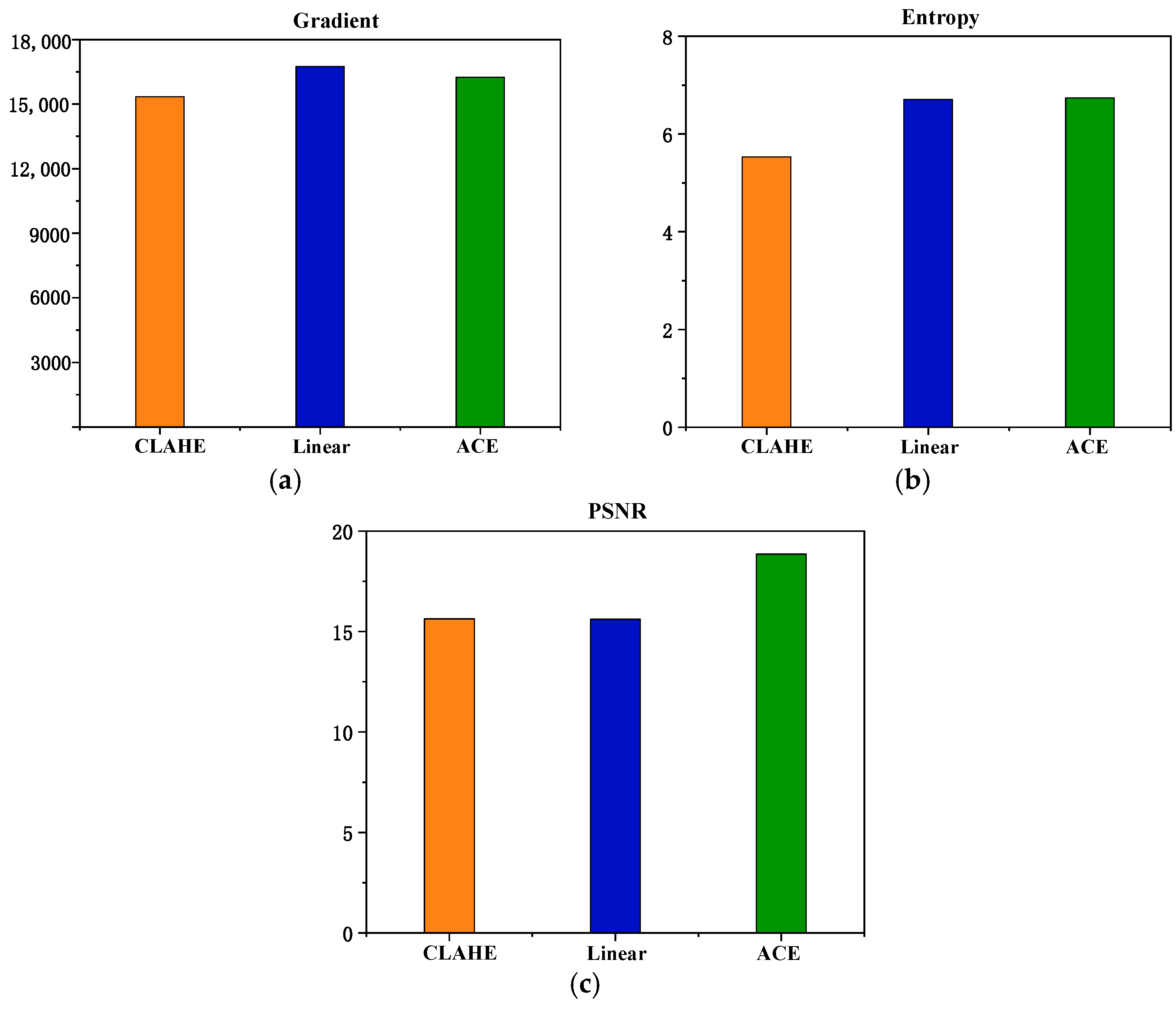
The above three indicators were calculated for the entire dataset by three data enhancement algorithms, and the results are shown in Figure 5. It can be seen that although the gradient of the image obtained by the linear transformation method is more significant, the entropy value is lower than that of the ACE method we used, and the image does not contain rich, detailed information. The peak signal-to-noise ratio of the CLAHE and linear methods is lower than that of the ACE method. Therefore, the ACE method used in this paper can better enhance the detailed information and gradient information of the image than the other two methods and can obtain more features for object detection.

3.3. Two-Level Multi-Vehicle Detection Network

This section mainly introduces the specific details of the two-level network. The first-level network mainly uses the improved YOLOv5s network to detect vehicles in the two-dimensional intensity image of lidar. The second-level network uses the 3D graph convolution network’s (3DGCN) point cloud classification network to further judge the suspicious areas in the first-level network to improve the detection accuracy of the object. The two-level detection network structure is shown in Figure 6.

3.3.1. Improved First-Level YOLO Network

YOLOv5 is the best-performing network of the YOLO series of networks in recent years, and it has made many improvements over the previous YOLOv3 [30] and YOLOv4 [31]. It improves the network structure and adds some image processing methods and training skills. The design of the network is mainly aimed at the visible image. The image’s color, texture, edge, and other features are extracted through the backbone network with multiple residual blocks stacked. However, most of the features learned by the network have grayscale information and there is no complex texture information of visible light images; thus, it is not ideal for the object detection task in a lidar intensity image. The complex feature extraction network only extracts more repeated features. Therefore, to reduce unnecessary operations, this study adopted the MobileNetv3 [32] lightweight feature extraction network as the backbone network of YOLOv5.
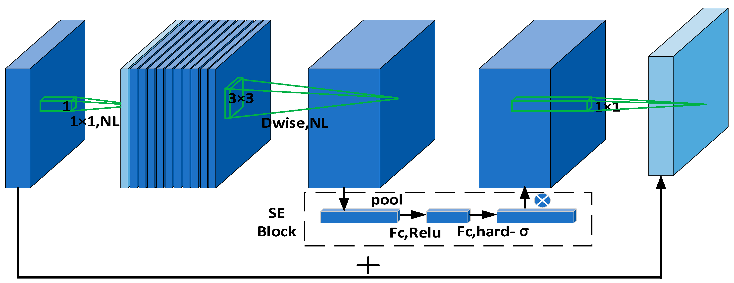
The MobileNetv3 network is further improved on the basis of the advantages of the Mo-bileNetv1 [33] and MobileNetv2 [34] network design. It adopts a combination of complementary search technologies, and the resource-constrained NAS (platform aware NAS) performs the module search. After each module is determined, the network layer performs a local search through netadapt to make fine adjustments. The h-swish activation function is introduced into the network structure. The MobileNetv3 network not only ensures accuracy but also greatly reduces the amount of network computing. The network module of MobileNetv3 is shown in Figure 7. NL is a linear activation function.
The structural parameters of the MobileNetv3-Small network used in this study are shown in Table 2.
Although the swish activation function can effectively improve the accuracy of the network, the amount of calculation of swish is too large. Therefore, using the h-swish (hard version of swish), the calculation is as follows:
h s w i s h [ x ] = x R e L U 6 ( x + 3 ) 6
where ReLU6 can avoid the loss of numerical accuracy, run fast, and promote the improvement of network accuracy.

3.3.2. Second-Level 3DGCN Network

This research was aimed at the long-distance detection of multiple weak and small vehicles by lidar. It used the two-dimensional intensity image information from the first-level detection, which causes many missed detection problems. Lidar point cloud data are a collection of vectors in a three-dimensional coordinate system. They not only represent the outer-surface shape and position information of an object, but also can represent the color information (RGB) and reflection intensity information (Intensity) of a point. They can make up for the lack of information in two-dimensional images. Due to the characteristics of the Gm-APD imaging principle, there is also echo information in the background, resulting in the excessive background noise of the point cloud data. Therefore, we did not directly use 3D point cloud data for object detection. In order to re-duce the interference of point cloud background noise, the suspicious area of the first-level network was mapped to the 3D point cloud area. In the second-level detection, the 3DGCN point cloud classification network [35] was introduced to make use of the 3D point cloud information of lidar to judge the missed object again.
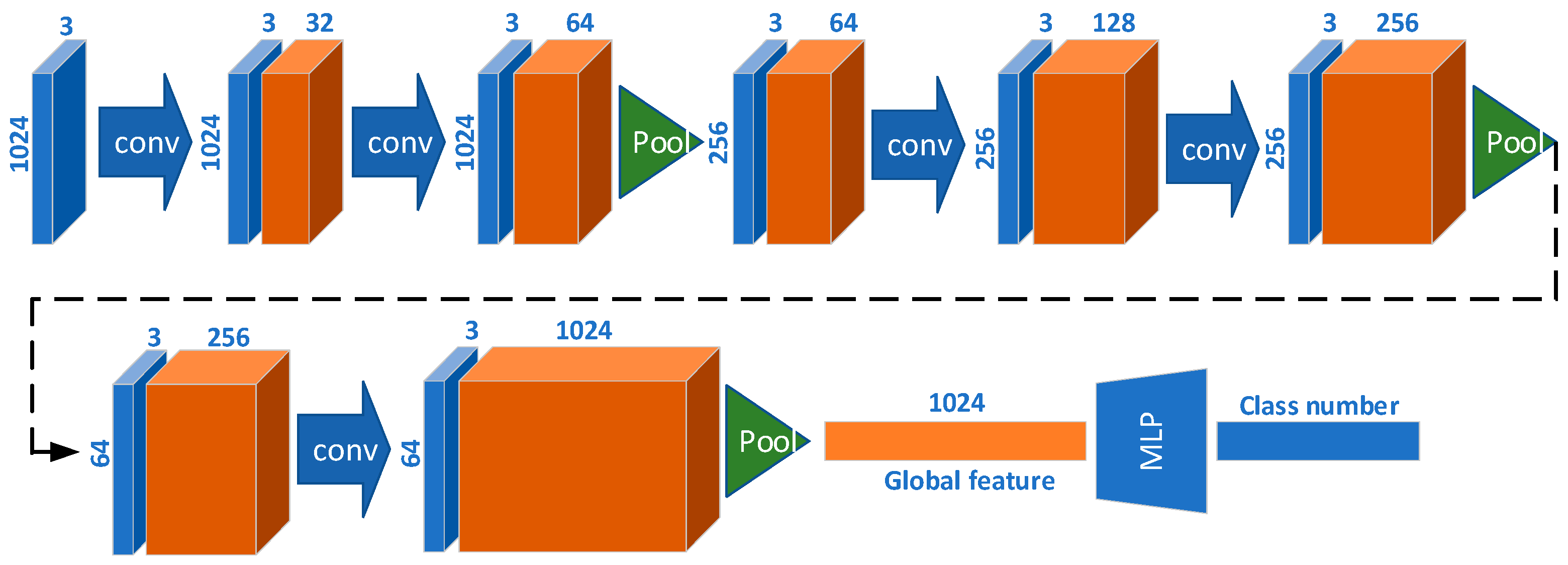
The 3DGCN network is a three-dimensional graph convolution network that extracts features from point cloud data and applies them to point cloud object classification. A point cloud instance is seen as a set containing N points P = { p n | n = 1 , 2 , , N } located on the surface of the object of interest. p n represents the nth point of this example, and its attributes can describe coordinates, normal vector, color and reflectivity information, etc. This study only uses the position information of the point cloud. That is, for p n = { x n , y n , z n } , the three-dimensional point cloud objects are represented by a matrix of size N × 3 as input to the network, and the output produces predicted output scores c for each class of interest. The network structure is shown in Figure 8.
3D point cloud data are an unordered collection of data points and no specific spatial 3D pattern can be observed; therefore, a learnable kernel is used in the 3DGCN.
(1)
Learnable kernel
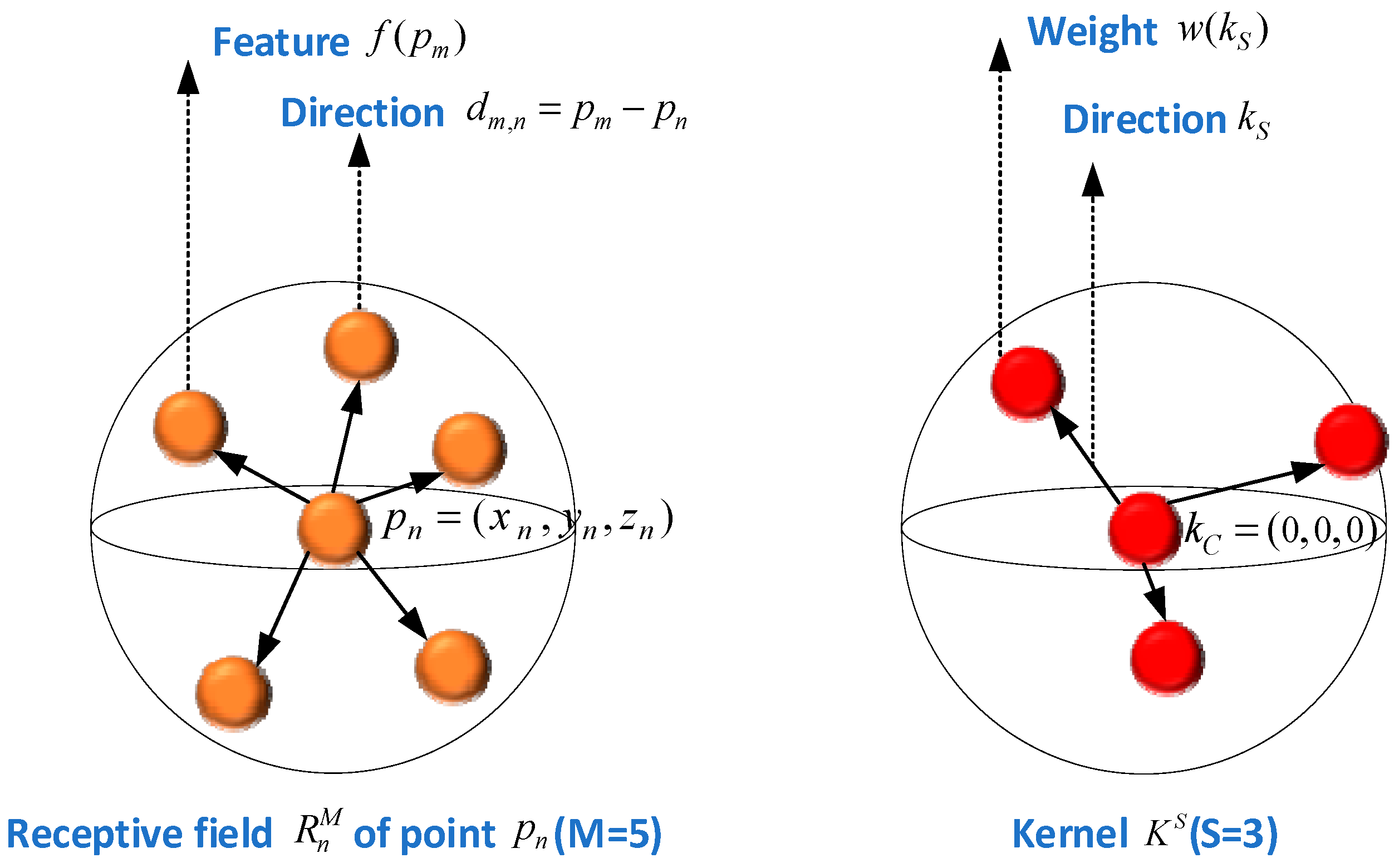
A 3D point cloud object with N points is denoted as P = { p n | n = 1 , 2 , , N } , p n 3 , and in order to describe the features of each point in the 3DGCN, the associated D-dimensional feature vector is represented by f ( p ) D . In order to obtain the local geometric information of the p n point, the three-dimensional receptive field of the p n point is determined by the set of M adjacent points. The receptive field R n M and the kernel K S graph are shown in Figure 9.
R n M is expressed as the receptive field of a point p n of size M:
R n M = p n , p m | p m N ( p n , M )
where N ( p n , M ) denotes the M nearest neighbors of p n based on distance p m p n , and the corresponding direction vector, which is used for the convolution calculation. The corresponding direction vector d m , n = p m p n is used for convolution calculation.
The 3D point cloud structure is convolved using the 3D graph convolution kernel K S , where S represents the number of supports in the kernel. K S consists of the S + 1 core point k j 3 , that is,
K S = { k C , k 1 , k 2 , , k S }
where k C = ( 0 , 0 , 0 ) is the center of the kernel, and k 1 to k S denote the relevant support.
(2)
3DGCN calculation
Unlike 2D convolution, this measures the features within the receptive field of p n (i.e., f ( p n ) , f ( p m ) , p m N ( p n , M ) , as defined in Equation (13)) and the weight of the kernel K S similarity between vectors. Centered on k C with S supports (i.e., w ( k C ) , w ( k S ) , s = 1 , 2 , , S ), consider all possible pairs between ( p m , k S ) . Therefore, Conv( R n M , K S ) in the 3DGCN is defined as:
C o n v ( R n M , K S ) = f ( p n ) , w ( k C ) + g ( A )
where represents the inner product operation, A = { s i m ( p m , k s ) | s ( 1 , S ) } , and sim is defined as:
s i m ( p m , k s ) = f ( p m ) , w ( k s ) d m , n , k s d m , n k s
The above formula yields the inner product between f ( p n ) and w ( k C ) based on cosine similarity. Function g in Equation (15) is the maximum similarity s i m ( p m , k S ) of each supported k S in the kernel. According to the above definition, the 3D graph convolution operation in the 3DGCN is calculated as:
C o n v ( R n M , K S ) = f ( p n ) , w ( k C ) + s = 1 S m a x m ( 1 , M ) s i m ( p m , k s )
Since the direction vector d m , n in Equation (17) is not a global coordinate, the 3DGCN model introduces a shift-invariant property. In Equation (16), the similarity function simply calculates the cosine similarity between d m , n and k S , regardless of their length. That is, the scale-invariant property is introduced.

3.3.3. Confidence Threshold Processing Method

By setting the confidence threshold judgment method, we can ensure the reliability of the detection performance and better improve the detection accuracy of small and weak objects.
First, by setting the confidence threshold of the first-level detection network for lidar intensity image object detection to θ 1 , and setting θ 1 to 0.85, the object with a confidence greater than or equal to 0.85 in the first-level detection is a reliable object. Result θ is between 0.5 and 0.85, and it is judged as a suspicious object. Then, the second-level point cloud classification is performed for the point cloud data corresponding to the position of the object frame, the object category score is obtained as the score, and the two-level result is comprehensively judged as the final second-level object confidence score:
c o n f = λ θ + ( 1 λ ) s c o r e
Finally, the reliable objects detected by the first-level network and the objects detected by the second-level network are combined together and outputted as the final result of the second-level detection.

4. Experimental Results and Analysis

4.1. Experimental Operating Environment

The hardware and software platforms used in the experiments were configured as follows: Intel (R) Core (TM) i7-8700 @3.20 GHz (CPU), NVIDIA 2080Ti 11GB (2 GPUs), Gloway DDR4 16GB (memory), Samsung 960 Pro 512GB (SSD), Ubuntu 18.04 (system), and Pytorch (deep learning framework).

4.2. Evaluation Indicators

In this study, we used a low-computational theoretical metric (BFLOP) to evaluate the size of the model, and the accuracy P (precision), the recall R (recall), the F1 score, and the average precision AP (average precision) to evaluate the detection of the model performance. The formula is as follows:
P = T P T P + F P
R = T P T P + F N
F 1 = 2 P R P + R
A P = 0 1 P ( R ) d R
where P is the precision rate, R is the recall rate, TP is the number of true positive samples, FP is the number of false positive samples, and FN is the number of false negative samples.

4.3. Network Training

In this experiment, 12 sets of data were collected, with a total of 6000 intensity images corresponding to 6000 point cloud data. Since this experiment collected dynamic data in continuous time for different distances and different scenes, the object changes in adjacent frames were small. Therefore, using as few training sets as possible can achieve better detection results. In the first-level two-dimensional object detection network, 1260 intensity images were used as the training set, 540 intensity images were used as the validation set, and 4200 intensity images were used for network testing. The second-level 3D point cloud network used the point cloud data corresponding to the first-level intensity images to train the network.
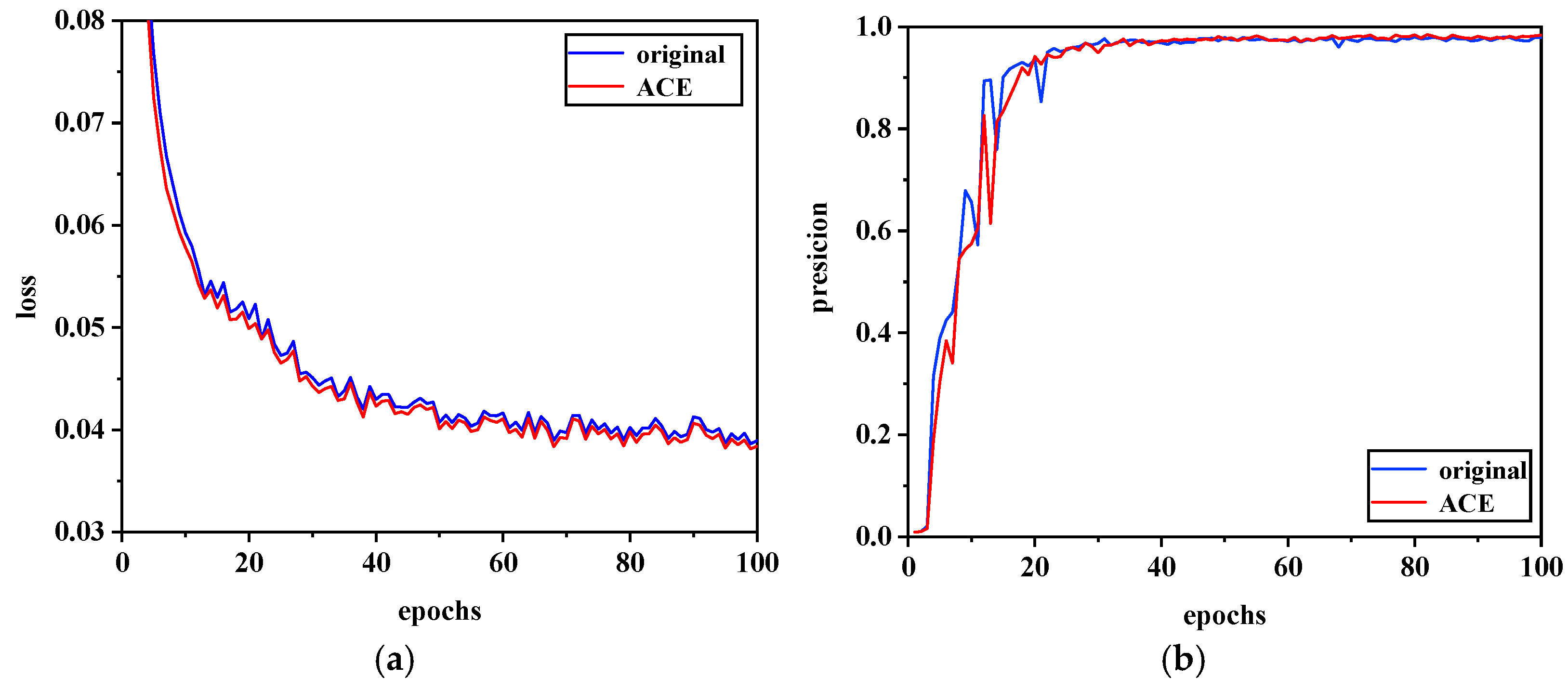
The parameters of the first-level network training were 100 epochs, the batch size was 32, and the initial learning rate was 0.01. The original and contrast-enhanced data were trained by the network, and the training results are shown in Figure 10a (the loss curve of training). Figure 10b is the epoch curve of training. It can be seen from Figure 10a that the loss curve during the training process using the ACE method decreases with the increase in epochs. When the epoch is 60, the loss drops to a position close to 0.04 and, finally, tends to be stable when the epoch is 100, which is when the model training results are the best. This curve can eventually obtain a lower loss value compared to the loss curve trained on the original data. It can be seen from Figure 10b that with the increase in epoch value in the training process of the ACE method, the curve change is relatively smooth compared with the original image training curve. Similarly, when the epoch is 60, the training accuracy begins to stabilize to 100, and the final training prescription value is higher than the original image.
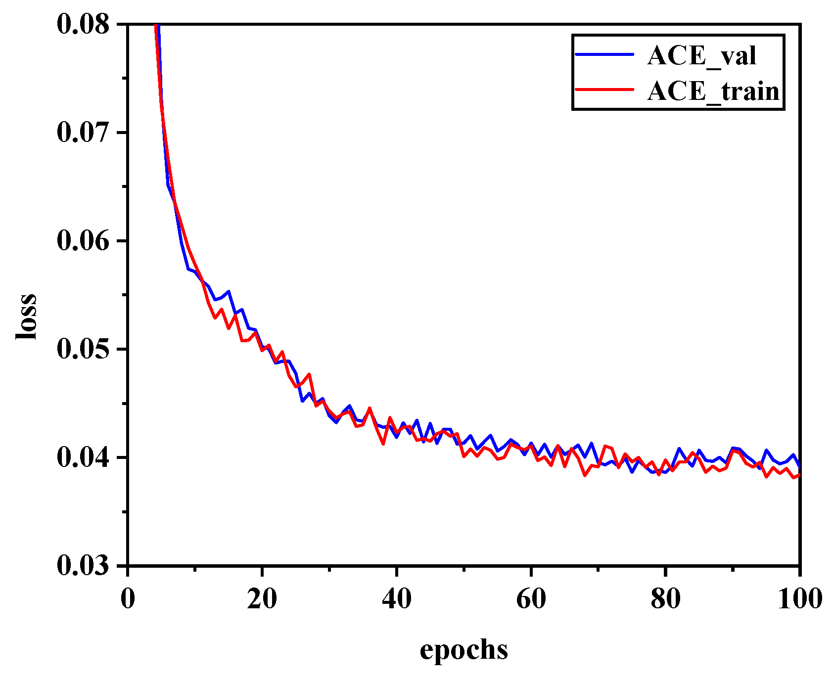
In order to verify the robustness and generalization of the model, the loss curve in the training process of the image enhanced by the ACE method is compared with the loss curve change in the verification process, as shown in Figure 11. It can be seen from the figure that the loss values of both the training set and the validation set decrease with the increase in the epoch value and tend to be stable at 100 epochs, and the training model has strong robustness.
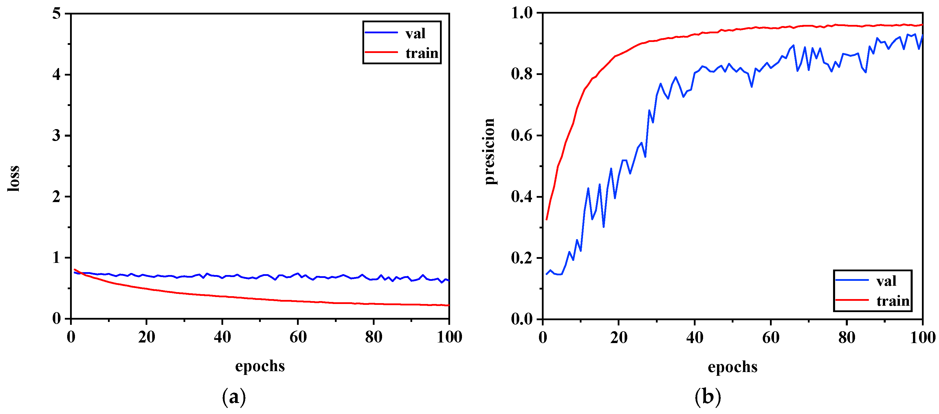
The training parameters for the second-level 3D point cloud network were set to epochs of 100 and a batch size of 16. The training results are shown in Figure 12. Figure 12a shows the loss change curve of the training set and the validation set during the training process. It can be seen that with the increase in training epochs, the loss value is constantly decreasing and tends to be stable. Figure 12b shows the precision change curve of the training set and the validation set during the training process. The curve increases with the increase in training epochs and, finally, achieves a better training result.

4.4. Test Results and Analysis

4.4.1. Comparison of First-Level Networks

Due to the two-level network used in this study for object detection, in order to avoid the redundant calculation of the two-level network, the first-level YOLOv5s network was optimized and improved, and its backbone network CSPDarknet was designed as a lightweight network to reduce the complexity of the network and improve the detection accuracy. In this study, MobileNetv3 was used as the backbone network, which has fewer parameters, less computation, and a shorter reasoning time, and introduces an attention mechanism as compared with CSPDarknet. Because of the high signal-to-noise ratio of the enhanced intensity image and prominent vehicle characteristics, the network can effectively learn the characteristics of the object. The parameters and structure of this network were compared with several other lightweight networks, as shown in Table 3.
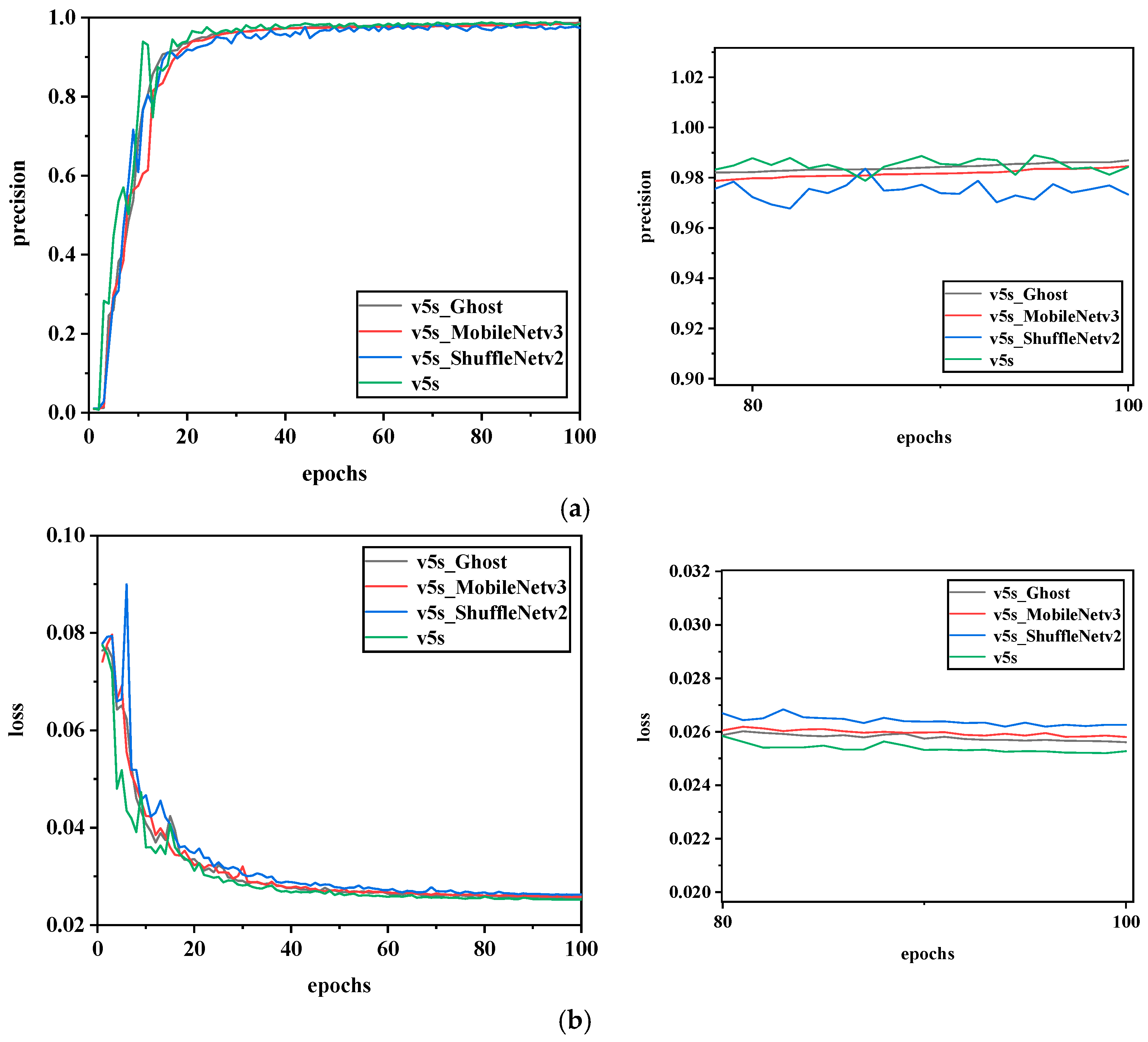
Table 3 shows that the number of network parameters optimized by using MobileNetv3 is only 3,542,756, which is more than half of the parameters compared with the original YOLOv5s, and the floating-point calculation is only 6.3 GFLOPs. The comparison of the training results of the above four different backbone networks is shown in Figure 13.
As shown in Figure 12a, the detection accuracy of different backbone networks varies with network training. It can be seen that the detection accuracy of the MobileNetv3 used by us is higher than that of YOLOv5s and ShuffleNetv2 when it tends to be stable. The change curve of the loss function in Figure 12b shows that the v5s_ MobileNetv3 network gradually becomes stable with the increase in the number of training times and, finally, can reach a lower loss value. Combining the analysis of the complexity of the network structure and the detection accuracy, we can conclude that v5s_MobileNetv3 has a better performance compared with several other networks. It not only has the lowest network complexity but also has a higher detection accuracy.
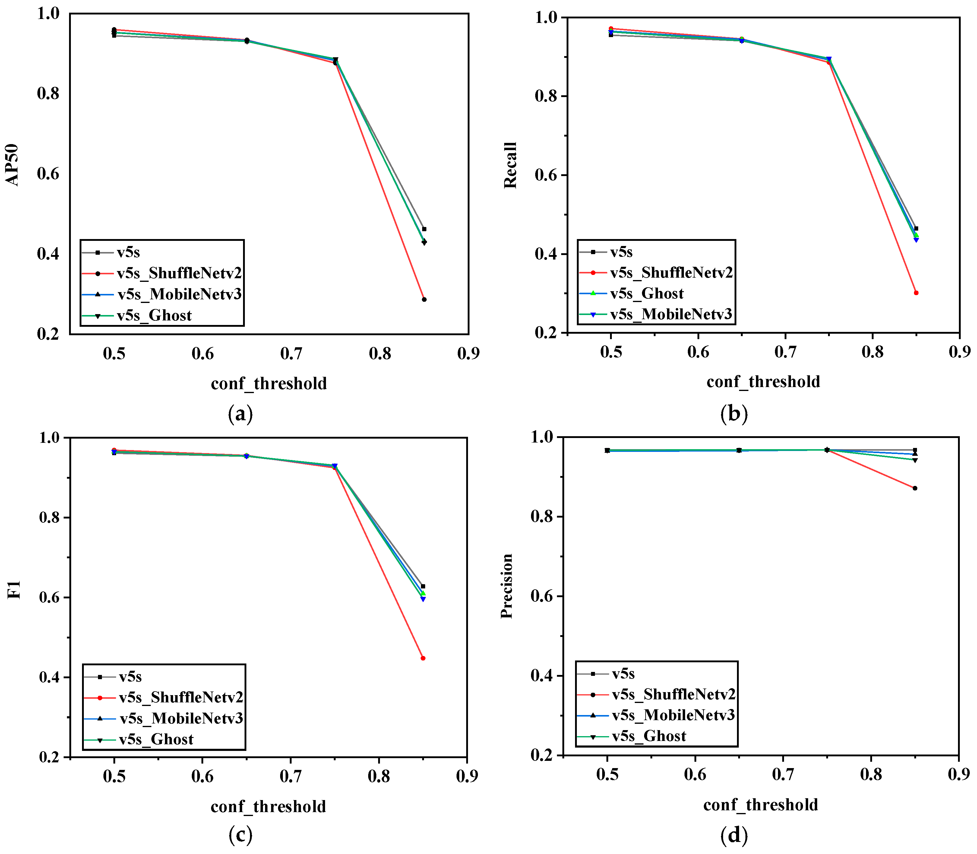
The confidence thresholds of the first-level network were set to 0.5, 0.65, 0.75, and 0.85. The comparison of the detection results of the four networks on 4200 test images is shown in Figure 14. The results of different networks at different confidence thresholds were compared by using four evaluation indexes. It can be seen that with the increase in confidence threshold, P, R, F1, and AP50 all decrease. When the threshold value is set to 0.85, the detection accuracy of the MobileNetv3 backbone network used in this study is 95.71%, 1.0% lower than v5s, and 1.4% and 8.5% higher than Ghost and Shufflenetv2, respectively. The recall rate was 44.70%, 1.0% lower than v5s, 1.0% higher than Ghost, and 14.5% higher than ShuffleNetv2. F1 is 60.9%, 1.8% lower than v5s, 1.2% higher than Ghost, and 16.1% higher than ShuffleNetv2. AP50 is 44.88%, 0.56% lower than v5s, 1.65% higher than Ghost, and 14.91% higher than ShuffleNetv2. The overall performance is significantly lower than when the confidence is 0.5. Although the accuracy of the detected objects is high, there are many missed objects, resulting in a low recall rate and a low AP50 value; thus, the objects cannot be accurately detected.
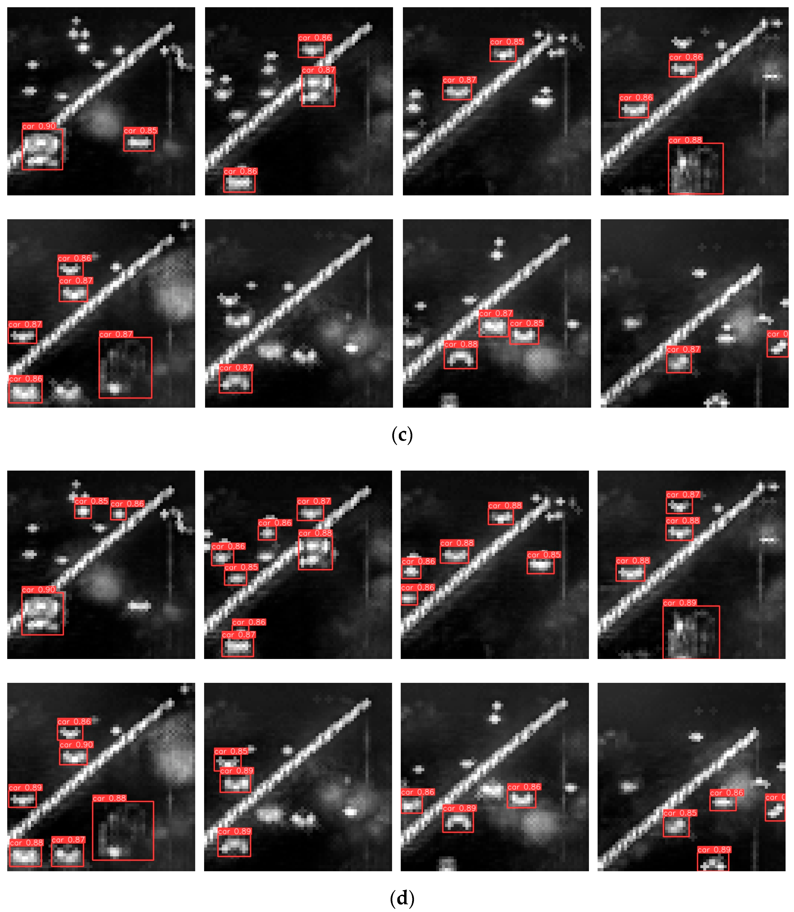
As the confidence thresholds of 0.5 and 0.65 shows little difference in the calculation of each index, AP50, AP75, AP85, and AP@50:5:95 of the four networks under the confidence thresholds of 0.5, 0.75, and 0.85 are shown in Table 4, as they can more objectively evaluate the performance of different networks. Based on the above indicators, although the performance of MobileNetv3 was slightly worse than that of v5s, the network performance used in this study was better at measuring the detection accuracy and model complexity. Figure 15 shows the partial detection results of the four methods with confidence levels greater than 0.85. It can be seen that there are still a lot of missed detections for small objects. Therefore, multiple objects cannot be accurately detected using only intensity images.

4.4.2. Comparison of Second-Level Networks

This study adopted a 2D object detection method for intensity images in the first-level network and set a confidence threshold of 0.85. The object with a first-level network detection result threshold greater than 0.85 was defined as a reliable object, and the object with a confidence threshold between 0.5–0.85 was defined as a suspicious object. A second-level point cloud classification network needs to be used for secondary identification of such suspicious objects. For our point cloud data, the number of point clouds varied significantly at different distances. Therefore, we used the 3DGCN point cloud classification network, which has good classification performance at present. This network can extract local 3D features from point clouds across scales, introduce translation and scale invariance, and use the graph maximum pool mechanism to define a learnable kernel.
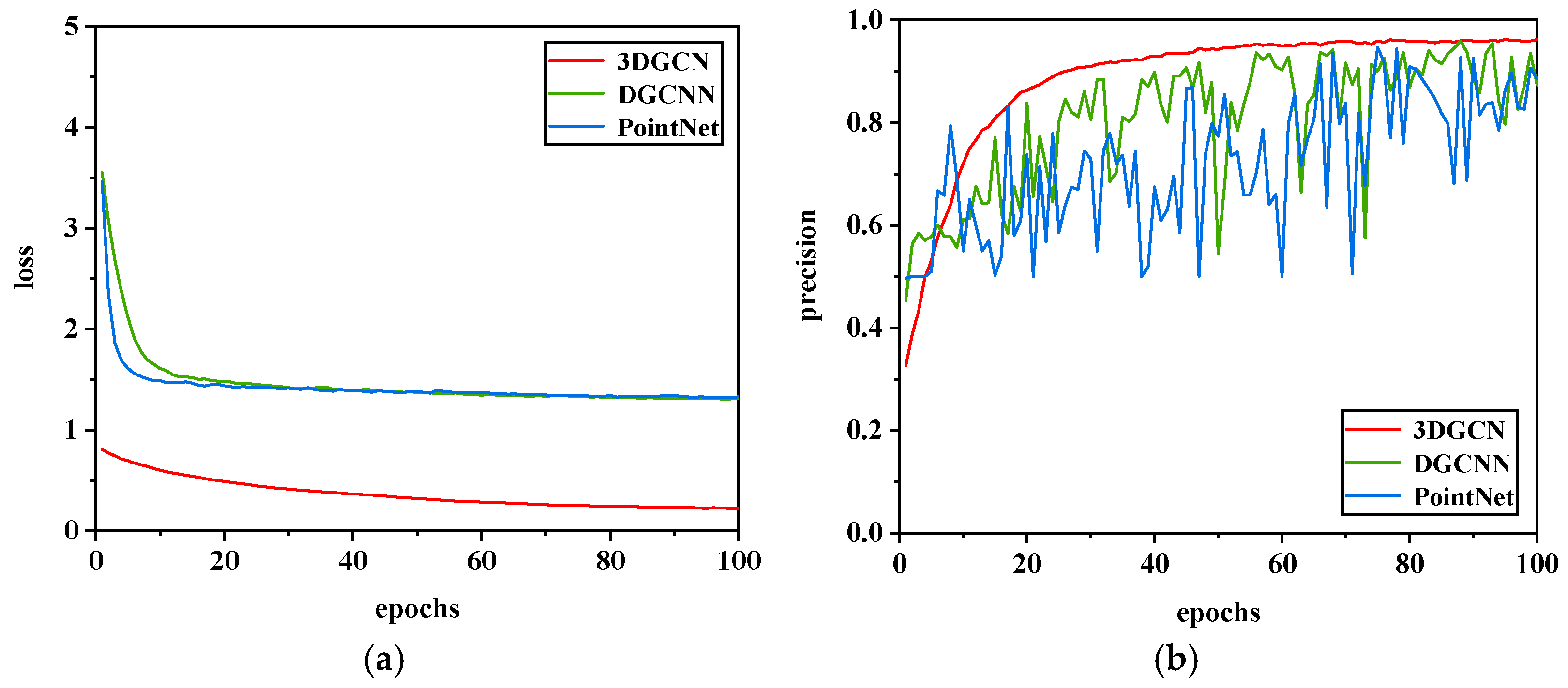
In order to verify the performance of the 3DGCN network, this network was compared with the current advanced point cloud classification dynamic graph convolutional neural network (DGCNN) [36] and PointNet [37] network. The training results of the different networks are shown in Figure 16.
As can be seen from Figure 16a, the accuracy of the 3DGCN network increases steadily with increasing epochs. The highest detection accuracy is 0.9625, 0.34% higher than the DGCNN network and 1.5% higher than the PointNet network. It can be seen from Figure 16b that the loss value of the 3DGCN network decreases with the increase in epochs and, finally, stabilizes at about 0.22. During the training process of the DGCNN and the PointNet network, the loss value decreases with the increase in epochs and, finally, stabilizes at about 1.3. Therefore, we used the 3DGCN network to train with higher accuracy, lower loss value, and better classification performance.

4.4.3. Comparison of Results between Single-Level Networks and Two-Level Networks

Since the single-level network only uses a single intensity image for multiple objects with high confidence, there are a lot of missed detections. Therefore, based on two-dimensional intensity image detection, point cloud data with the three-dimensional spatial structure of the object were introduced, and 3D convolution was used for the vehicle point cloud data through the graph neural network to learn the similar features around the object. Moreover, finally, the score of the object category was outputted. In the first-level network, the confidence threshold was set to 0.85. Since this study focused on 2D detection, the 3D recognition reidentified suspicious areas from the 2D detection, and λ in Equation (18) was set to 0.6. Finally, the two-level detection results were combined into the final detection results. As shown in Table 5, the single-level 2D network was trained for 100 epochs, and the second-level 3D network was trained for 100 epochs. Under the condition that the first-level IOU threshold is 0.85, compared with the single-level network, AP50, AP75, AP85, and AP@50:5:95 increased by 52.5%, 52.48%, 50.54%, and 52.06%, respectively. Therefore, the two-level network can effectively improve the accuracy of object detection significantly.
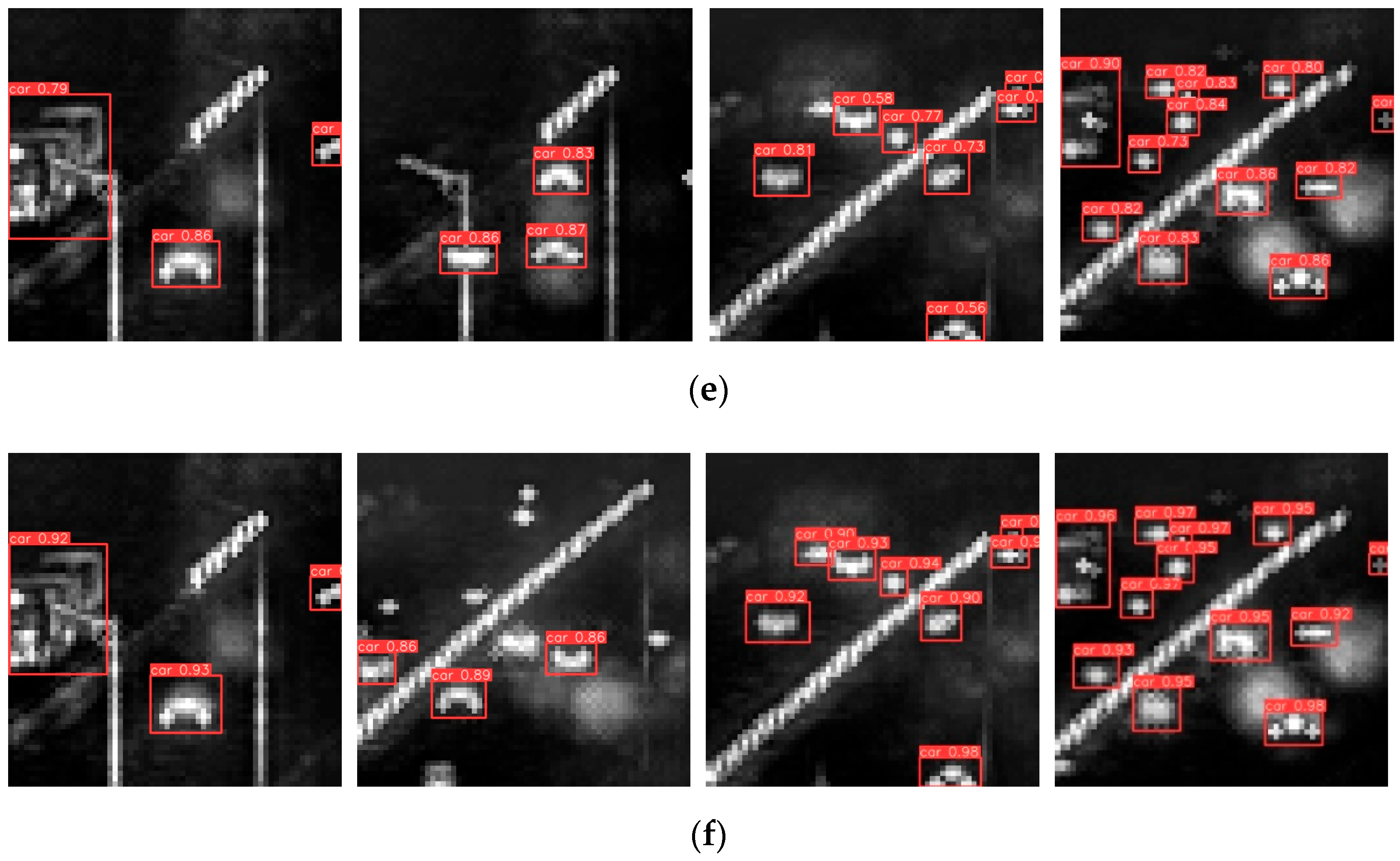
Next, the method proposed in this paper was compared with the state-of-the-art 2D object detection methods [38,39,40,41,42]. The comparison results are shown in Table 6. It can be seen that our method was compared with the other five object detection algorithms. The training time is short, and with the increase in the IOU threshold, the AP value is relatively stable; therefore, the algorithm has strong robustness and better performance than the other five methods. The detection results of the six methods are shown in Figure 17, which shows that our method has good detection performance for weak and small objects.
In order to verify the low complexity of the algorithm proposed in this paper, the weight of this algorithm was compared with the current advanced object detection method using 3D point cloud data directly [43,44,45] and the advanced 2D object detection algorithm. The results are shown in Figure 18.
It can be seen from Figure 18 that the weight size of the Point-Voxel RCNN (PV-RCNN) is 50M, and there are many network training parameters. Currently, in the advanced 3D point cloud object detection network, the complexity of the PointPillars network is low, and the weight size is 23 M. Among the advanced 2D object detection networks, the Faster RCNN network has higher complexity, with a weight size of 315 M. The YOLOX network has lower complexity, with a weight size of 68.5 M. However, we propose that the weight of the two-level object detection network is 12 M. The algorithm complexity is lower than other object detection networks, and the network performance is better.

5. Conclusions

Multi-vehicle object detection at night has essential practical value in military operations. Gm-APD lidar images have different echo intensities of objects at different distances, where the contrast of long-distance intensity images is weak, the object is tiny, and the missed detection rate is high in dense object images. Only a single two-dimensional image cannot accurately detect the object. We proposed a two-level deep learning object detection method for 2D intensity images and 3D point cloud data. By selecting YOLOv5s as the first-level 2D detection network framework and improving it, the MobileNetv3 network was introduced as the backbone network, compressing the network model and improving the detection accuracy of small objects by using the attention mechanism. The confidence threshold value was set in the first-level network, and the object higher than the threshold value was reserved. The suspicious object lower than the threshold value was converted into the corresponding point cloud data. The 3DGCN network was used to identify the point cloud object, and the suspicious object’s 2D and 3D detection results were used as the detection results of the object. Finally, the 2D and 3D network detection results were merged to obtain the final result. The experimental results show that the accuracy of the model proposed in this paper, AP@50:5:95, is 0.9638, which is about 20% higher than other networks. The training time is shorter, and the network has better robustness. This study comprehensively evaluated the superiority of the proposed method, which has practical significance for the research of lidar vehicle detection at night. In future studies, we will build richer datasets for different weather and objects, and deeply explore new research methods and application scenarios.

Author Contributions

Conceptualization, Y.D. and D.D.; methodology, Y.D.; software, Y.D.; investigation, H.Z.; data curation, D.D. and Y.J.; writing—original draft preparation, Y.D.; writing—review and editing, Y.D.; supervision, Y.Q.; project administration, J.S. All authors have read and agreed to the published version of the manuscript.

Funding

This research received no external funding.

Data Availability Statement

Not applicable.

Conflicts of Interest

The authors declare no conflict of interest.

References

  1. Qin, P.; Cai, Y.L.; Liu, J.; Fan, P.R.; Sun, M.H. Multilayer Feature Extraction Network for Military Ship Detection From High-Resolution Optical Remote Sensing Images. IEEE J. Sel. Top. Appl. Earth Obs. Remote Sens. 2021, 14, 11058–11069. [Google Scholar] [CrossRef]
  2. Janakiramaiah, B.; Kalyani, G.; Karuna, A.; Prasad, L.V.N.; Krishna, M. Military object detection in defense using multi-level capsule networks. Soft Comput. 2021, 1–15. [Google Scholar] [CrossRef]
  3. Zhang, W.Y.; Fu, X.H.; Li, W. The intelligent vehicle object recognition algorithm based on object infrared features combined with lidar. Comput. Commun. 2020, 155, 158–165. [Google Scholar] [CrossRef]
  4. Cossio, T.K.; Slatton, K.C.; Carter, W.E.; Shrestha, K.Y.; Harding, D. Predicting Small Object Detection Performance of Low-SNR Airborne Lidar. IEEE J. Sel. Top. Appl. Earth Obs. Remote Sens. 2010, 3, 672–688. [Google Scholar] [CrossRef]
  5. Kechagias-Stamatis, O.; Aouf, N.; Richardson, M.A. 3D automatic object recognition for future LIDAR missiles. IEEE Trans. Aerosp. Electron. Syst. 2016, 52, 2662–2675. [Google Scholar] [CrossRef] [Green Version]
  6. Silva, L.G.D.; Cerqueira, S., Jr. A LiDAR Architecture Based on Indirect ToF for Autonomous Cars. J. Microw. Optoelectron. Electromagn. Appl. 2021, 20, 504–512. [Google Scholar] [CrossRef]
  7. Sheu, M.H.; Morsalin SM, S.; Zheng, J.X.; Hsia, S.C.; Lin, C.J.; Chang, C.Y. FGSC: Fuzzy guided scale choice SSD model for edge AI design on real-time vehicle detection and class counting. Sensors 2021, 21, 7399. [Google Scholar] [CrossRef]
  8. De-Las-Heras, G.; Sánchez-Soriano, J.; Puertas, E. Advanced driver assistance systems (ADAS) based on machine learning techniques for the detection and transcription of variable message signs on roads. Sensors 2021, 21, 5866. [Google Scholar] [CrossRef]
  9. Caban, J.; Nieoczym, A.; Dudziak, A.; Krajka, T.; Stopková, M. The Planning Process of Transport Tasks for Autonomous Vans—Case Study. Appl. Sci. 2022, 12, 2993. [Google Scholar] [CrossRef]
  10. Ma, Y.; Anderson, J.; Crouch, S.; Shan, J. Moving object detection and tracking with doppler LiDAR. Remote Sens. 2019, 11, 1154. [Google Scholar] [CrossRef] [Green Version]
  11. Liu, D.; Sun, J.F.; Gao, S.; Ma, L.; Jiang, P.; Guo, S.H.; Zhou, X. Single-parameter estimation construction algorithm for Gm-APD ladar imaging through fog. Opt. Commun. 2021, 482, 126558. [Google Scholar] [CrossRef]
  12. Qiu, C.R.; Sun, J.F.; Zhou, X.; Jiang, P.; Li, C.C.; Wang, Q. Experimental research on polarized LIDAR imaging based on GM-APD. In Optics Frontier Online 2020: Optics Imaging and Display; SPIE: Bellingham, WA, USA 2020, 11571, 40–50. [Google Scholar]
  13. Wang, P.; Fan, E.; Wang, P. Night vehicle object recognition based on fuzzy particle filter. J. Intell. Fuzzy Syst. 2020, 38, 3707–3716. [Google Scholar] [CrossRef]
  14. Hu, H.N.; Zhu, M.; Li, M.Y.; Chan, K.L. Deep Learning-Based Monocular 3D Object Detection with Refinement of Depth Information. Sensors 2022, 22, 2576. [Google Scholar] [CrossRef] [PubMed]
  15. Mendez, J.; Molina, M.; Rodriguez, N.; Cuellar, M.P.; Morales, D.P. Camera-LiDAR Multi-Level Sensor Fusion for Object Detection at the Network Edge. Sensors 2021, 21, 3992. [Google Scholar] [CrossRef] [PubMed]
  16. Kim, K.; Kim, C.; Jang, C.; Sunwoo, M.; Jo, K. Deep learning-based dynamic object classification using LiDAR point cloud augmented by layer-based accumulation for intelligent vehicles. Expert Syst. Appl. 2021, 167, 113861. [Google Scholar] [CrossRef]
  17. Huang, D.Y.; Zhou, Z.H.; Deng, M.; Li, Z.H. Nighttime vehicle detection based on direction attention network and bayes corner localization. J. Intell. Fuzzy Syst. 2021, 41, 783–801. [Google Scholar] [CrossRef]
  18. Kuang, H.L.; Zhang, X.S.; Li, Y.J.; Chan, L.L.H.; Yan, H. Nighttime vehicle detection based on bio-inspired image enhancement and weighted score-level feature fusion. IEEE Trans. Intell. Transp. 2016, 18, 927–936. [Google Scholar] [CrossRef]
  19. Mo, Y.Y.; Han, G.Q.; Zhang, H.D.; Xu, X.M.; Qu, W. Highlight-assisted nighttime vehicle detection using a multi-level fusion network and label hierarchy. Neurocomputing 2019, 355, 13–23. [Google Scholar] [CrossRef]
  20. Chen, L.; Hu, X.M.; Xu, T.; Kuang, H.L.; Li, Q.Q. Turn signal detection during nighttime by cnn detector and perceptual hashing tracking. IEEE Trans. Intell. Transp. 2017, 18, 3303–3314. [Google Scholar] [CrossRef]
  21. Li, S.X.; Bai, P.F.; Qin, Y.F. Dynamic Adjustment and Distinguishing Method for Vehicle Headlight Based on Data Access of a Thermal Camera. Front. Phys. 2020, 8, 354. [Google Scholar] [CrossRef]
  22. Cai, Y.F.; Zhang, T.T.; Wang, H.; Li, Y.C.; Liu, Q.C.; Chen, X.B. 3D vehicle detection based on lidar and camera fusion. Automot. Innov. 2019, 2, 276–283. [Google Scholar] [CrossRef]
  23. Wang, H.; Zhang, X.D. Real-time vehicle detection and tracking using 3D LiDAR. Asian J. Control 2021, 24, 1459–1469. [Google Scholar] [CrossRef]
  24. Tian, Y.F.; Song, W.; Chen, L.; Fong, S.; Sung, Y.; Kwak, J. A 3D Object Recognition Method from LiDAR Point Cloud Based on USAE-BLS. IEEE Trans. Intell. Transp. Syst. 2022, 1–11. [Google Scholar] [CrossRef]
  25. McCulloch, J.; Green, R. Conductor Reconstruction for Dynamic Line Rating Using Vehicle-Mounted LiDAR. Remote Sens. 2020, 12, 3718. [Google Scholar] [CrossRef]
  26. Zhou, Q.Y.; Tan, Z.W.; Yang, C.C. Theoretical limit evaluation of ranging accuracy and power for LiDAR systems in autonomous cars. Opt. Eng. 2018, 57, 096104. [Google Scholar] [CrossRef]
  27. Ma, L.; Sun, J.F.; Jiang, P.; Liu, D.; Zhou, X. Signal extraction algorithm of Gm-APD lidar with low SNR return. Optik 2020, 206, 164340. [Google Scholar] [CrossRef]
  28. Du, H.C. Image Denoising Algorithm Based on Nonlocal Regularization Sparse Representation. IEEE Sens. J. 2019, 20, 11943–11950. [Google Scholar] [CrossRef]
  29. Xiang, Q.; Peng, L.K.; Pang, X.L. Image DAEs based on residual entropy maximum. IET Image Processing 2020, 14, 1164–1169. [Google Scholar] [CrossRef]
  30. Redmon, J.; Farhadi, A. YOLOv3: An Incremental Improvement. arXiv 2018, arXiv:1804.02767. [Google Scholar]
  31. Bochkovskiy, A.; Wang, C.Y.; Liao, H.Y.M. YOLOv4: Optimal speed and accuracy of object detection. arXiv 2020, arXiv:2004.10934. [Google Scholar]
  32. Howard, A.; Sandler, M.; Chu, G.; Chen, L.C.; Chen, B.; Tan, M.X.; Wang, W.J.; Zhu, Y.K.; Pang, R.M.; Vasudevan, V.; et al. Searching for mobilenetv3. In Proceedings of the IEEE/CVF International Conference on Computer Vision, Seoul, Korea, 27–28 October 2019; pp. 1314–1324. [Google Scholar]
  33. Howard, A.G.; Zhu, M.; Chen, B.; Kalenichenko, D.; Wang, W.J.; Weyand, T.; Andreetto, M.; Adam, H. Mobilenets: Efficient convolutional neural networks for mobile vision applications. arXiv 2017, arXiv:1704.04861. [Google Scholar]
  34. Sandler, M.; Howard, A.; Zhu, M.L.; Zhmoginov, A.; Chen, L.C. MobileNetV2: Inverted Residuals and Linear Bottlenecks. In Proceedings of the IEEE Conference on Computer Vision and Pattern Recognition, Salt Lake City, UT, USA, 23 June 2018. [Google Scholar]
  35. Lin, Z.H.; Huang, S.Y.; Wang, Y.C.F. Convolution in the Cloud: Learning Deformable Kernels in 3D Graph Convolution Networks for Point Cloud Analysis. In Proceedings of the IEEE/CVF Conference on Computer Vision and Pattern Recognition, Seattle, WA, USA, 14–19 June 2020; pp. 1800–1809. [Google Scholar]
  36. Wang, Y.; Sun, Y.; Liu, Z.; Sarma, S.E.; Bronstein, M.M.; Solomon, J.M. Dynamic Graph CNN for Learning on Point Clouds. ACM Trans. Graphic. 2018, 38, 1–12. [Google Scholar] [CrossRef] [Green Version]
  37. Qi, C.R.; Su, H.; Mo, K.; Guibas, L.J. PointNet: Deep Learning on Point Sets for 3D Classification and Segmentation. In Proceedings of the IEEE Conference on Computer Vision and Pattern Recognition, Honolulu, HI, USA, 21–26 July 2017; pp. 652–660. [Google Scholar]
  38. Ren, S.; He, K.; Girshick, R.; Sun, J. Faster R-CNN: Towards Real-Time Object Detection with Region Proposal Networks. arXiv 2015, arXiv:1506.01497. [Google Scholar] [CrossRef] [PubMed] [Green Version]
  39. Liu, W.; Anguelov, D.; Erhan, D.; Szegedy, C.; Reed, S.; Fu, C.Y.; Berg, A.C. SSD: Single shot multibox detector. In Computer Vision—ECCV 2016; Springer: Cham, Switzerland, 2016; pp. 21–37. [Google Scholar]
  40. Lin, T.Y.; Goyal, P.; Girshick, R.; He, K.; Doll´ar, P. Focal loss for dense object detection. In Proceedings of the IEEE International Conference on Computer Vision, Venice, Italy, 22–29 October 2017; pp. 2980–2988. [Google Scholar]
  41. Zhou, X.; Wang, D.; Krähenbühl, P. Objects as points. arXiv 2019, arXiv:1904.07850. [Google Scholar]
  42. Ge, Z.; Liu, S.; Wang, F.; Li, Z.; Sun, J. YOLOX: Exceeding yolo series in 2021. arXiv 2021, arXiv:2107.08430. [Google Scholar]
  43. Yan, Y.; Mao, Y.; Li, B. SECOND: Sparsely Embedded Convolutional Detection. Sensors 2018, 18, 3337. [Google Scholar] [CrossRef] [Green Version]
  44. Lang, A.H.; Vora, S.; Caesar, H.; Zhou, L.; Yang, J.; Beijbom, O. Pointpillars: Fast encoders for object detection from point clouds. In Proceedings of the IEEE/CVF Conference on Computer Vision and Pattern Recognition, Long Beach, CA, USA, 15–20 June 2019; pp. 12697–12705. [Google Scholar]
  45. Shi, S.; Guo, C.; Jiang, L.; Wang, Z.; Shi, J.; Wang, X.; Li, H. PV-RCNN: Point-Voxel Feature Set Abstraction for 3D Object Detection. In Proceedings of the IEEE/CVF Conference on Computer Vision and Pattern Recognition, Seattle, WA, USA, 13–19 June 2020; pp. 10529–10538. [Google Scholar]
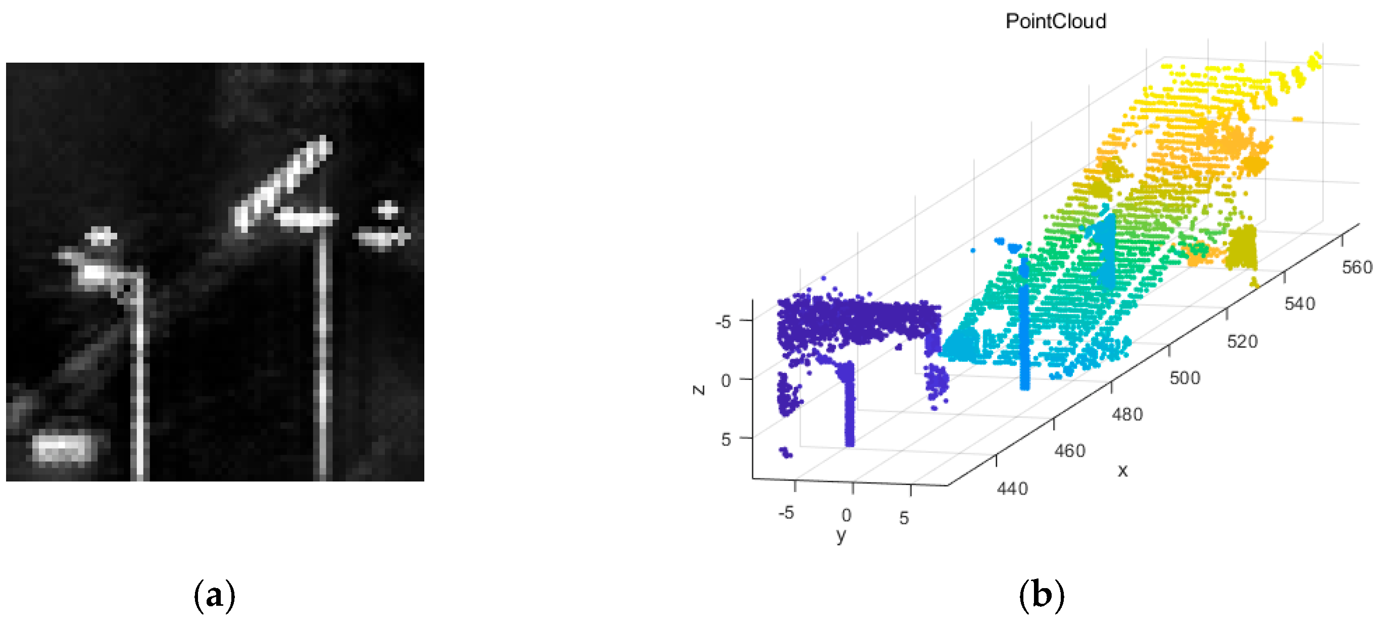
Figure 1. Lidar data. (a) Intensity image; (b) point cloud data.
Remotesensing 14 03553 g001
Figure 2. Data acquisition scenario.
Remotesensing 14 03553 g002
Figure 3. Small object data in the dataset. (a) Small objects with a minimum of 8 pixels; (b) small objects with a minimum of 5 pixels.
Remotesensing 14 03553 g003
Figure 4. Intensity image-enhanced 3D visualization results: (a) 2D intensity image; (b) 2D intensity image; (c) 3D results enhanced by the ACE method; (d) 3D results enhanced by the ACE method; (e) 3D results enhanced by the linear transformation method.
Remotesensing 14 03553 g004aRemotesensing 14 03553 g004b
Figure 5. Comparison of three data augmentation algorithms. (a) Gradient; (b) entropy; (c) PSNR.
Remotesensing 14 03553 g005
Figure 6. Two-level detection network structure.
Remotesensing 14 03553 g006
Figure 7. MobileNetv3 network module structure.
Remotesensing 14 03553 g007
Figure 8. 3DGCN network structure.
Remotesensing 14 03553 g008
Figure 9. Receptive field R n M and kernel KS graph.
Remotesensing 14 03553 g009
Figure 10. The curve of the training process of the first-level network on the original data and the data processed by the ACE method. (a) Loss curve of training; (b) precision curve of training.
Remotesensing 14 03553 g010
Figure 11. The loss curve of the first-level network in the training process of the original data and the data processed by the ACE method.
Remotesensing 14 03553 g011
Figure 12. The curve changes of training set and validation set during the training of 3D point cloud network. (a) Loss curve; (b) precision curve.
Remotesensing 14 03553 g012
Figure 13. The loss and precision curves of 3D point cloud network training. (a) Precision curve of training; (b) loss curve of training.
Remotesensing 14 03553 g013
Figure 14. Comparison of test results of different networks (confidence thresholds are 0.5, 0.65, 0.75 and 0.85). (a) AP50; (b) recall; (c) F1; (d) precision.
Remotesensing 14 03553 g014
Figure 15. Detection results of different networks. (a) YOLOv5s detection result (conf ≥ 0.85); (b) YOLOv5s_Ghost detection result (conf ≥ 0.85); (c) YOLOv5s_ShuffleNetv2 detection result (conf ≥ 0.85); (d) YOLOv5s_MobileNetv3 detection result (conf ≥ 0.85).
Remotesensing 14 03553 g015aRemotesensing 14 03553 g015b
Figure 16. Different point cloud classification network training results. (a) Loss curve; (b) precision curve.
Remotesensing 14 03553 g016
Figure 17. Test results of four methods. (a) Faster R-CNN; (b) SSD; (c) RetinaNet; (d) CenterNet; (e) YOLOX; (f) Ours.
Remotesensing 14 03553 g017aRemotesensing 14 03553 g017b
Figure 18. Comparison of network weight size of different object detection algorithms.
Remotesensing 14 03553 g018
Table 1. Night vehicle data details.
TimeNumber of Image FramesMaximum Number of Objects per FrameMinimum
Object Ratio
Image Minimum Object Pixel Count
20:37:19500153.052 × 10−58
20:37:58500113.052 × 10−58
20:38:11500121.907 × 10−55
20:38:2450061.907 × 10−55
20:52:09500111.907 × 10−55
20:52:2250093.052 × 10−58
20:52:37500173.052 × 10−58
20:52:51500161.907 × 10−55
21:22:4850083.052 × 10−58
21:23:0550082.670 × 10−57
21:23:2450073.052 × 10−58
21:23:5050072.670 × 10−57
Table 2. MobileNetv3-Small network structure parameters.
InputOperatorExp SizeOutSENLs
6402 × 3bneck, 3 × 3-16-HS2
3202 × 24bneck, 3 × 31616RE2
1602 × 24bneck, 3 × 37224-RE2
802 × 24bneck, 3 × 38824-RE1
802 × 40bneck, 5 × 59640HS1
402 × 40bneck, 5 × 524040HS1
402 × 40bneck, 5 × 512048HS1
402 × 48bneck, 5 × 514448HS1
402 × 96bneck, 5 × 528896HS2
202 × 96bneck, 5 × 557696HS1
Table 3. Comparison of parameters of different lightweight network structures.
ModelLayersParametersGFLOPsWeight Size
YOLOv5s270 7,235,38916.5 13.7 MB
YOLOv5s_Shufflenetv2308 3,844,193 8.1 7.68 MB
YOLOv5s_Ghost453 3,897,605 8.8 7.50 MB
Ours340 3,542,756 6.37.17 MB
Table 4. Comparison results of AP values of different networks with different confidence thresholds.
APv5sv5s_ShuffeNetv2v5s_GhostOurs
Conf = 0.5
AP500.96820.97490.97220.9751
AP750.96820.97480.97180.9749
AP850.96820.97400.96920.9744
AP@50:5:950.95460.95960.95320.9540
Conf = 0.75
AP500.90470.89630.91430.9116
AP750.90470.89630.91410.9115
AP850.90470.89630.91270.9115
AP@50:5:950.89380.88570.89910.8944
Conf = 0.85
AP500.45440.29970.43230.4488
AP750.45440.29970.43230.4488
AP850.45440.29970.43230.4488
AP@50:5:950.45100.29830.42820.4432
Table 5. Two- level detection results.
Epochs_2DEpochs_3Dconf_thresdAP50AP75AP85AP@50:5:95
Ours1001000.850.97380.97360.95420.9638
Table 6. Comparison results with other methods.
Epochs_AllAP50AP75AP85AP@50:5:95Train Time
Faster R-CNN2000.92040.80440.72390.76396.5 h
SSD2000.95900.87700.86300.79505.4 h
RetinaNet2000.96750.81300.81140.77005.2 h
CenterNet2000.96800.8030.79100.76813.2 h
YOLOX2000.97910.8860.77000.71762.8 h
Ours2000.97380.97360.95420.96383.8 h
Publisher’s Note: MDPI stays neutral with regard to jurisdictional claims in published maps and institutional affiliations.