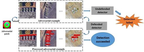
A Cascade Defense Method for Multidomain Adversarial Attacks under Remote Sensing Detection

Abstract

Deep neural networks have been widely used in detection tasks based on optical remote sensing images. However, in recent studies, deep neural networks have been shown to be vulnerable to adversarial examples. Adversarial examples are threatening in both the digital and physical domains. Specifically, they make it possible for adversarial examples to attack aerial remote sensing detection. To defend against adversarial attacks on aerial remote sensing detection, we propose a cascaded adversarial defense framework, which locates the adversarial patch according to its high frequency and saliency information in the gradient domain and removes it directly. The original image semantic and texture information is then restored by the image inpainting method. When combined with the random erasing algorithm, the robustness of detection is further improved. Our method is the first attempt to defend against adversarial examples in remote sensing detection. The experimental results show that our method is very effective in defending against real-world adversarial attacks. In particular, when using the YOLOv3 and YOLOv4 algorithms for robust detection of single-class targets, the AP60 of YOLOv3 and YOLOv4 only drop by 2.11% and 2.17%, respectively, under the adversarial example.

1. Introduction

With the development of earth observation technology, the resolution of earth observation devices is increasing, which makes it possible for earth observation devices to use deep learning technology to detect specific targets [1,2,3]. Using optical remote sensing images to detect targets can identify the location and class information of ground targets in different environments, and even calculate the attitude information of earth observation devices according to the invariant target characteristics. As a result, the earth observation task plays an important role in target detection [4,5], battlefield situation analysis [6] and other fields.

However, recent work has shown that deep neural networks are vulnerable to adversarial examples [7,8,9,10,11]. In particular, by adding invisible noise to images, the deep learning model can be misled with high confidence. However, most of the current adversarial attack forms are carried out in the digital domain [8,11,12]. Due to lighting, angle, distance, camera and other reasons [13,14], the adversarial examples in the digital domain cannot be transferred to the physical domain. In the past, adversarial examples in the digital domain were limited to changes in the pixel values but not the number of pixels. However, some recent studies have shown that by modifying the pixel value of a certain area in the image, the deep learning model can also be misled. Such adversarial examples are called adversarial patch. Based on this idea, Brown et al. [14] incorporated the idea of expectation beyond transformation (EOT) into the adversarial example generation step. They then successfully applied the adversarial patch in the digital domain to the physical domain, and attacked the classifier. Then, Liu et al. [15] used an adversarial patch to attack the detector, and the generated adversarial patch could effectively attack YOLOv2 and Faster R-CNN. Subsequently, many studies on adversarial examples were carried out in the physical domain, including attacking detection targets such as pedestrians, road signs, faces, and vehicles [16,17,18,19,20,21,22,23,24]. The existence of adversarial examples makes the neural network face huge security risks in practical applications. Hence it is necessary to build a defense method against the threat of adversarial examples.

Early adversarial defense work focused on the defense of adversarial examples in the digital domain, such as JPEG compression [25,26], denoising networks [27,28], defensive distillation [29,30], adversarial example detection [31,32,33] and other methods. Among them, adversarial training [34] is an effective defense method for digital adversarial examples to enhance the robustness of the model. There are many studies on defense methods, but these methods are not effective under the attack of adversarial examples in the physical domain. For example, if adversarial training is performed on the detector, the adversarial training will consume a large amount of computing resources and will cause the performance of the detector to drop severely under clean examples [35]. Adversarial examples in the physical domain mostly attack in the form of adversarial patches, which is different from the mainstream attack methods in the digital domain. An adversarial patch is a patch formed in a regular shape, such as a circle or a rectangle, and it is restricted to be within the $l_2-\mathrm{norm}$ or $l_{\infty }-\mathrm{norm}$ ball of radius $ϵ$. An adversarial patch is one form of adversarial example, and the attack can be launched simply by attaching to the detection target. There has been no work so far that considers how to defend against adversarial patch attacks in the detection task of optical remote sensing. Our work proposes a robust defense framework for this problem for the first time and conducts robust defense tests against the adversarial patch designed in recent related work. We first utilize the features of the adversarial patch to propose a localization technique that can discover and remove adversarial patches from natural images. Based on the removed area, we use deep learning-based image inpainting technology to inpaint the missing area, and we use the random erasing algorithm to compensate for the performance degradation caused by image inpainting. The results show that our method exhibits strong robustness against adversarial attacks in air-to-ground target observations. The conceptual framework of our algorithm is shown in Figure 1:

Our contributions are as follows:

• To the best of our knowledge, we are the first to propose an effective defense method against adversarial attacks on optical remote sensing detection including but not limited to earth observation satellite detection of ground targets, aerial target detection of drones to the ground, etc. Our method can effectively defend against vanishing attacks of adversarial patches attached to or near the detection target.
• We propose a framework for defense against adversarial patches, including adversarial patch positioning, image inpainting, and feature learning enhancement methods for adversarial patches. This makes our defense framework robust against adversarial attacks.
• A series of experiments demonstrate the effectiveness of our algorithm, including the defense capabilities of different models with multiple types of adversarial patches. Our experiments show that our framework can provide strong robustness to object detection models under different detectors and different adversarial attacks.

2. Related Work

This section summarizes some related work on adversarial attacks and defenses.

2.1. Adversarial Attack

The adversarial examples for deep neural networks can be divided into the digital domain and physical domain attacks. The concept of adversarial examples in the digital domain was first proposed by Szegedy et al. [7], who revealed the vulnerability of deep neural networks to adversarial examples. Goodfellow et al. [8] proposed a fast gradient sign method (FGSM) algorithm, which is a noniterative algorithm that can quickly generate adversarial examples against the classifier. Later, Madry et al. [11] proposed an iterative attack algorithm, called projected gradient descent (PGD), and pointed out that the PGD attack is the strongest attack algorithm generated by using the local first-order information of the network. In fact, the PGD algorithm is the most commonly used adversarial example generation method in adversarial training algorithms. Researchers have performed much research on the generation of adversarial examples in the digital domain, such as JSMA [36], One Pixel Attack [10], C&W attack [12], Universal Adversarial Perturbations [37], etc. Although these algorithms can effectively attack classifiers or detectors in the digital domain, they cannot migrate to the physical domain due to lighting, shooting angle and distance, camera pixels, etc. Kurakin et al. [37] printed digital adversarial examples and then used the Inception V3 classifier to classify them. Their experiments showed that digital adversarial examples are still aggressive in the physical domain, but their aggressiveness decreases significantly, which can be caused by the shooting angle or distance [38]. To generate more robust adversarial examples in the physical world, Sharif et al. [39] generated more robust adversarial examples in the real world by incorporating a nonprintability score and a total variation loss in the process of generating adversarial examples. At present, most of the adversarial attacks in the physical domain are carried out using adversarial patches. For example, Wu et al. [19] attached an adversarial patch to clothing, which could evade detection by the detector, and Thys et al. [22] also performed similar work. Increasingly, adversarial patches are being used to attack diverse targets. Avoiding detection, deceiving models, and modifying object properties are all goals of the attack.

2.2. Adversarial Attack for Aerial Image Detection

The development of adversarial example technology enables adversarial examples to effectively attack remote sensing detection. Den et al. [16] successfully evaded object detection in aerial images based on the YOLO algorithm using the generated adversarial examples. Wang et al. [21] used a dual attention attack to generate adversarial examples, namely, model attention and human attention, and attached them to the vehicle, which could make the vehicle evade detection by the latest detectors. Du et al. [40] considered factors such as atmosphere and material properties in the process of generating adversarial examples and printed the adversarial examples into the physical world for testing. Research on adversarial examples for attacking aerial image detection is still limited, but the current technology can effectively attack aerial image detection.

2.3. Physical Domain Adversarial Defense

For adversarial examples in the digital domain, there are many defense methods [25,26,27,28,29,30,31,32,33], but these methods all show robust vulnerability in the face of the newly proposed adversarial attack algorithm. At present, only adversarial training methods have not been completely defeated and have been proven to be the most effective methods against digital adversarial examples [34]. However adversarial training is not suitable for adversarial examples in the physical domain. On the one hand, adversarial training is very time-consuming, and on the other hand, adversarial training will lead to a decrease in the accuracy of the model for clean examples [35]. Hence current research has gradually shifted to studying how to defend against physical adversarial examples. Naseer et al. [41] mitigated the influence of adversarial patches on the model by regularizing the gradients of the noisy regions. Hayes et al. [42] located adversarial examples by constructing a saliency map of the image using guided backpropagation and erasing them. However, [43] pointed out that the above two defense methods can be overcome by approximating the gradient or incorporating a smoothing step in backpropagation. Xiang et al. [44] adopted neural networks with small receptive fields to limit the number of features corrupted by adversarial patches and employed robust masking as a secure aggregation mechanism to ensure model robustness. The above three methods are all for the defense of the classifier but they cannot be effectively transferred to the detector. Bao et al. [45] observed that the objectness score of the detection target was slightly higher than the background and used the objectness regularization method to enhance the objectness score of the detection target. This method can effectively improve the performance of the detector in vanishing attacks. However, if the adversarial patch is attached to small targets, this method will fail. We note that, to date, the problem of defense against adversarial examples in detection tasks based on optical remote sensing images has not been studied. Thus, our method is the first to pursue this research direction.

3. Problem Definition

We first define the adversarial attack and defense problems studied in this paper.

3.1. The Purpose of the Attacker

In this paper, we mainly study the defense method against vanishing attacks based on adversarial examples in the physical domain. The purpose of the vanishing attack is to attach the adversarial patch to the detection target or near the detection target in order to avoid detection by the detector. Define the detector model as $D_{\theta }(·)$, where $\theta$ is the model parameter, the adversarial patch as $P_{adv}$, the clean image as x, the ground-truth bounding box of the corresponding target in the image is $Tob{j}_i$, and i is the i-th detection target in the detection image. Let the adversarial patch be attached to the corresponding area of the target in the clean image, so the clean image attacked by the adversarial patch is defined as $app(x,P_{adv})=x^{*}$, and the final vanishing attack is defined as:

$$\begin{array}{cc}\hfill & D_{\theta }\left(x^{*}\right)\cap Tob{j}_i=⌀\hfill \\ \hfill & s.t.d(x,x^{*})\le ϵ\hfill \end{array}$$

(1)

where the distance matrix $d(·)$ is expressed as $l_2-\mathrm{distance}$ $d(x,x^{*})={∥x-x^{*}∥}_2^2$ or $l_{\infty }-\mathrm{distance}$ $d(x,x^{*})={∥x-x^{*}∥}_{\infty }$, and the perturbation is restricted to be within the $p-\mathrm{norm}$ ball of radius $ϵ$ to quantify the distance between two inputs x and $x^{*}$ that are small enough. Actually, $ϵ$ makes the adversarial patch look more natural. It can be seen from the above formula that the adversarial patch can achieve the purpose of vanishing attack by making the detector unable to identify and detect the detection target.

3.2. The Purpose of the Defender

The defender uses preprocessing or the model robustness enhancement method to defend against adversarial attacks. Among them, the white-box attack is the most aggressive adversarial attack method. Effective defense against white-box attacks can also be robust to black-box attacks to a certain extent, but not vice versa. The purpose of the defender is to ignore the influence of the adversarial patch on the model under the white-box attack and restore the detection performance of the model before being attacked. Robust detector detection needs to guarantee the following:

1.

The detector should try to restore the detection ability of the detection image under the adversarial attack;

2.

When not attacked by adversarial examples, it is necessary to ensure that the performance of the detector on the clean detection image does not degrade;

Define the robust detector model as $R{D}_{\theta }\left(x^{*}\right)$ and the predicted bounding box of the detector for clean images as $Pob{j}_i$. Robust detection can be expressed as follows:

$$\begin{array}{cc}\hfill & R{D}_{\theta }\left(x^{*}\right)\cap Pob{j}_i\approx R{D}_{\theta }\left(x^{*}\right)\cap Tob{j}_i\hfill \\ \hfill & s.t.R{D}_{\theta }\left(x\right)\approx Tob{j}_i\hfill \end{array}$$

(2)

3.3. Adversarial Patch

The adversarial patch defined by Equation (1) will cause the attack in the physical domain to fail due to light, shooting angle and other reasons. The generation technique of the adversarial patch introduced the idea of expectation over transformation (EoT) to generate a robust adversarial patch so that it can be used to attack in the physical domain. Brown et al. [14] proposed the patch application operator $A(p_{adv},x,l,r,s)$ to generate an adversarial patch, where l represents position change, r represents random change, and s represents scale change. In the process of adversarial patch generation, A is used to perform a set of transformations, and the final optimization goal of the vanishing attack is to minimize the detector output objectness score of the detection target bounding box. We define the objectness score as $L_{obj}$. The adversarial patch generated by this method has no other constraints on the pixels in the digital domain, thus the pixels in the adversarial patch do not have any connection with other pixels, and it will easily introduce high-frequency noise.

To make the adversarial attack effective in the physical domain, the subsequent adversarial patch generation methods all incorporate $NPS$ and $TV$ loss. The $NPS$ loss can make the adversarial patch to be printed out. The $NPS$ loss is defined as follows:

$$L_{nps}=\sum _{{\mathit{p}}_{pacth}\in {\mathit{p}}_{adv}}\underset{{\mathit{c}}_{print}\in \mathit{c}}{min}{∥{\mathit{p}}_{pacth}-{\mathit{c}}_{pacth}∥}_2$$

(3)

where ${\mathit{p}}_{patch}$ is all the pixel values in the adversarial patch ${\mathit{P}}_{adv}$, and ${\mathit{c}}_{patch}$ are all the pixel values of the pixel $\mathit{C}$ that can be printed out by the printer. $TV$ loss can prevent the patch from becoming a noisy image and ensure a smooth transition between adjacent pixels of the patch, and the $TV$ loss is defined as:

$$L_{tv}=\sum _{a,b}\sqrt{{({\mathit{p}}_{a,b}-{\mathit{p}}_{a+1,b})}^2+{({\mathit{p}}_{a,b}-{\mathit{p}}_{a,b+1})}^2}$$

(4)

where a and b are the pixel values ${\mathit{p}}_{a,b}$ at the pixel position $(a,b)$ of the adversarial patch ${\mathit{p}}_{adv}$. It should be noted that the image has three RGB color channels, and the $TV$ loss is calculated separately on these three channels. The adversarial patch can be optimized using $L_{obj}$, $L_{nps}$ and $L_{tv}$ losses:

$$L_{final}=\alpha L_{obj}+\beta L_{nps}+\phi L_{tv}$$

(5)

where $\alpha$, $\beta$, and $\phi$ are all hyperparameters. The $NPS$ loss restricts the color of the adversarial patch, and the pixel color can only be the color that can be printed by the printer. The $TV$ loss makes the region transition smoother. Although the $TV$ loss and $NPS$ loss make the adversarial patch avoid becoming a noise region, the $NPS$ loss limits the color of the adversarial patch while the $TV$ loss makes the adversarial patch show a regional color transition, which makes the adversarial patch also salient in the gradient domain, as shown in Figure 2e.

4. Defense Method

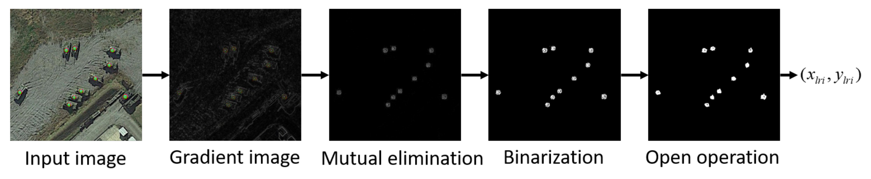
4.1. Locating Adversarial Patch

When attacking the optical remote sensing detection task, the adversarial patch will introduce salient features. For example, the adversarial examples for aerial image detection proposed in [16,40] have similar characteristics. Naseer et al. [41] have shown that adversarial examples with high frequency noise can be localized in the gradient domain. Hence we mainly consider the problem of localization of adversarial examples with salient features. Although [43] pointed out that incorporating a smoothing step to generate an adversarial example during backpropagation can reduce the gradient information of the adversarial example. Since the remote sensing detection tasks are all from a bird’s-eye view and the detection target area occupies a small proportion of the entire image, considering weather, air quality, etc., adversarial examples need sufficient salient features to make the attack effective. Therefore, according to this feature, we first locate the adversarial patch, then use the image inpainting technology based on deep learning to inpaint the image of the attacked area, and finally use the random erasing data augmentation method to improve the detection performance of the model under weak features.

We first compute the magnitude of the first-order gradients of the image based on the features of the adversarial examples:

$$\begin{array}{c}\hfill ∥\nabla x(a,b)∥=\sqrt{{\left(\frac{\partial x}{\partial a}\right)}^2+{\left(\frac{\partial x}{\partial b}\right)}^2}\end{array}$$

(6)

where a and b represent the horizontal and vertical directions of the image plane, and the gradient map is calculated on RGB channels. For subsequent processing, the gradient map is normalized to $[0,1]$:

$$\begin{array}{c}\hfill g\left(x\right)=\frac{∥\nabla x(a,b)∥-{∥\nabla x(a,b)∥}_{min}}{{∥\nabla x(a,b)∥}_{max}-{∥\nabla x(a,b)∥}_{min}}\end{array}$$

(7)

We find that, unlike natural images, adversarial patches usually require strong color channel information or contain enough high-frequency noise information to make them effective for attack. As shown in Figure 2, different from natural images, the adversarial patch can successfully attack in the physical domain, so it shows regional color transition. Figure 2e shows the gradient image of the regional color transition. The transition from a colored area to a colorless area will be displayed as colored lines. This feature is not available in natural images, and such strong color transitions are difficult to come by in a natural environment. In Figure 2f,g, the white lines in the gradient image are the gradient of the actual environment, which is caused by the unobvious separation of RGB channels. The regional color transition is caused by the introduction of the $TV$ loss. If the $TV$ loss is not introduced, the adversarial patch will degenerate into a noise patch, and the noise patch will fail to attack due to the loss of noise information under remote sensing detection. This feature allows the adversarial patch to have greater gradient information in the color transition region when they are transformed into the gradient domain. The RGB channels of the gradient map of the adversarial patch do not interfere with each other, while the natural images are different. Such strong gradient information of the adversarial patch will become more significant when normalizing the image, while the salience of the background will be further suppressed. Therefore, we locate the adversarial patch using this feature.

To reduce the saliency of the background area that is not attached to the adversarial patch, according to the nonoverlapping RGB channel gradient of the adversarial patch, we use separate RGB channels for mutual elimination. Defining the RGB channels of the gradient map $g\left(x\right)$ as $g{\left(x\right)}_R$, $g{\left(x\right)}_G$, and $g{\left(x\right)}_B$, the image $g{\left(x\right)}_e$ after background mutual elimination can be defined as:

$$\begin{array}{c}\hfill g{\left(x\right)}_e=\overrightarrow{\left|g{\left(x\right)}_R-g{\left(x\right)}_G\right|}+\overrightarrow{\left|g{\left(x\right)}_B-g{\left(x\right)}_G\right|}+\overrightarrow{\left|g{\left(x\right)}_B-g{\left(x\right)}_R\right|}\end{array}$$

(8)

where $\overrightarrow{\left|·\right|}$ represents the absolute value of the elements in the matrix. After the mutual elimination operation, the adversarial patch can be greatly separated from the background image, but there are still other background noises in the environment. Thus, it is necessary to further enhance the saliency of the adversarial patch and further suppress the background noise:

$$\begin{array}{c}\hfill g{\left(x\right)}_e=\frac{\left({(g{\left(x\right)}_e+\beta )}^{\alpha }\right)-{\left({(g{\left(x\right)}_e+\beta )}^{\alpha }\right)}_{min}}{{\left({(g{\left(x\right)}_e+\beta )}^{\alpha }\right)}_{max}-{\left({(g{\left(x\right)}_e+\beta )}^{\alpha }\right)}_{min}}\end{array}$$

(9)

Since $g\left(x\right)$ is normalized to $[0,1]$, from Equation (8) we can know that ${\left(g{\left(x\right)}_e\right)}_{max}\le 3$, for most background, ${\left(g{\left(x\right)}_e\right)}_{max}\ll 1$, this is because the gradient image of the natural image in the RGB channel will be greatly reduced after elementwise subtraction. For part of the adversarial patch ${\left(g{\left(x\right)}_e\right)}_{min}>1$, this is due to the nonoverlapping RGB channel gradient image of the adversarial patch; this feature can be used for saliency enhancement, where $\beta$ is the normalized pixel offset, its role is to prevent larger pixel values from dominating, generally greater than 1, and $\alpha$ is the magnification, its function is to enlarge the saliency of the adversarial patch and reduce the saliency of the background area, generally greater than 2.

After the saliency enhancement, the saliency of the adversarial patch in the detection image will be greatly enhanced. We threshold the image to filter out the background and obtain the position of the adversarial patch in the image. Since there may be some high-frequency noise with small areas in the detection image, it is necessary to use the open operation to eliminate the high-frequency noise in the small area; that is, the image is first corroded and then expanded. The expression is as follows:

$$\begin{array}{c}\hfill open\left(g\left(x\right)\right)=dilate(erode(g\left(x\right),{kernel}_1),{kernel}_2)\end{array}$$

(10)

kernel₁ and kernel₂ represent the size of the convolution kernel. We hope to eliminate high-frequency noise in a very small area during the erosion operation, so kernel₁ generally chooses a smaller convolution kernel, and during the expansion operation, we hope to connect adjacent pixel regions in the adversarial patch together, so kernel₂ chooses a larger convolution kernel.

Finally, the image coordinates of the upper left corner and the lower right corner of the rectangular block formed by the connected regions are selected, and the regions smaller than the threshold of the number of connected pixels in the region are eliminated. The remaining regions are the regions contaminated by the adversarial patch.

The adversarial patch positioning process is shown in Figure 3.

4.2. Image Inpainting and Data Augmentation

In previous work on the classifier adversarial patch defense problem, if the adversarial patch can be effectively located, the direct removal of the adversarial patch can have good defensive performance, or use traditional image inpainting techniques to reduce the impact of removal operations on prediction results. However, for aerial image detection tasks, directly removing adversarial patches may cause a huge drop in detection performance. This is mainly because the adversarial patch may be attached to the detection target, and removing the adversarial patch will cause the loss of texture and target semantic information. Figure 4 is a comparison figure before and after directly removing the adversarial patch. The detector is YOLOv3, and the IoU is set to 0.3. It can be seen that removing the adversarial patch causes a huge drop in detection performance.

Hayes et al. [42] proposed a fast image inpainting method for adversarial patches [46]. However, this method cannot effectively inpaint the texture information and high-level semantic information of objects, and the farther the inpainted area is from the edge, the worse the inpainting performance, as shown in Figure 5. This image inpainting algorithm is based on the traditional algorithm proposed by Telea et al. [46].

Therefore, image inpainting techniques are crucial for the detector to recover the detection performance of images. Image inpainting technology based on deep learning can complete tasks that traditional image inpainting technology cannot. On the one hand, image inpainting technology based on deep learning can inpaint the inpainting area of any shape, and on the other hand, it can inpaint the texture information and semantic information of the inpainting area. Compared with traditional image inpainting algorithms, deep learning-based image inpainting algorithms can generate more natural images.

In this paper, we use a coarse-to-fine image inpainting structure proposed by Yu et al. [47] to inpaint the image. It should be noted that other deep learning-based image inpainting techniques are also applicable to our framework.

The coarse-to-fine network architecture adopts a two-step network structure; that is, the first network performs the initial coarse prediction, and the second network takes the coarse prediction structure as input and refines the coarse prediction results.

The coarse prediction network is trained with reconstruction loss, while the fine network is jointly trained with reconstruction loss and GAN loss. The fine network can learn better texture and detail features, which is more conducive to image inpainting. The structure is shown in Figure 6.

The overall structure of the generative adversarial network is still used in the coarse-to-fine network. That is, the generator is used to generate the inpainted area, and then the discriminator is used to determine the image quality after image inpainting. The discriminator discriminates the area of the inpainted part and the whole image after inpainting to maintain the rationality of the inpainted area and the consistency of the whole image. The WGAN-GP loss is used in the global and local output of the refinement stage together with the reconstruction loss to optimize the model end-to-end.

Different from the original GAN, the WGAN uses the Earth-Mover(EM) distance to measure the distance between the input data distribution and the generator-generated data distribution, that is, the Wessertein-1 distance, which is expressed as follows:

$$\begin{array}{c}\hfill W(P_r,P_g)=\underset{\gamma \in \prod (P_r,P_g)}{inf}{\mathbb{E}}_{(x,y)\sim \gamma }\left[∥x-y∥\right]\end{array}$$

(11)

where $P_r$ is the true distribution of the input data, $P_g$ is the data distribution generated by the generator, and $\prod (P_r,P_g)$ is the set of all possible joint distributions that combine $P_r$ and $P_g$. Since solving the EM distance directly is highly intractable, the Kantorovich–Rubinstein duality theory can be used to transform the problem into solving the following equation:

$$\begin{array}{c}\hfill W({\mathbb{P}}_r,{\mathbb{P}}_w)=\underset{{∥f∥}_L\le 1}{sup}{\mathbb{E}}_{x\sim {\mathbb{P}}_r}\left[f\left(x\right)\right]-{\mathbb{E}}_{x\sim {\mathbb{P}}_w}\left[f\left(x\right)\right]\end{array}$$

(12)

The above formula shows that the upper bound of ${\mathbb{E}}_{x\sim {\mathbb{P}}_r}\left[f\left(x\right)\right]-{\mathbb{E}}_{x\sim {\mathbb{P}}_w}\left[f\left(x\right)\right]$ can be obtained for all functions f that satisfy the 1-Lipschitz restriction. Formula (12) can be approximated by solving the following formula:

$$\begin{array}{c}\hfill \underset{w:{∥f_{\theta }∥}_L\le 1}{max}{\mathbb{E}}_{x\sim {\mathbb{P}}_r}\left[f_{\theta }\left(x\right)\right]-{\mathbb{E}}_{x\sim {\mathbb{P}}_w}\left[f_{\theta }\left(x\right)\right]\end{array}$$

(13)

The above formula can be optimized by using the neural network method. The final optimization goal of the WGAN is as follows:

$$\begin{array}{c}\hfill \underset{G}{min}\underset{D\in \mathcal{D}}{max}{\mathbb{E}}_{x\sim P_r}\left[D\left(x\right)\right]-P_{z\sim \mathbb{P}\left(z\right)}\left[D\left(G\left(z\right)\right)\right]\end{array}$$

(14)

where $\mathcal{D}$ is the set of 1-Lipschitz functions. z is the input to the generator, sampled from a Gaussian or uniform distribution.

WGAN-GP improves WGAN by adding a penalty term as follows:

$$\begin{array}{c}\hfill \lambda {\mathbb{E}}_{\widehat{x}\sim P\left(\widehat{x}\right)}{({∥{\nabla }_{\widehat{x}}D\left(\widehat{x}\right)∥}_2-1)}^2\end{array}$$

(15)

where $P\left(\widehat{x}\right)$ samples uniformly along straight lines between points sampled from distributions $P_r$ and $p_g$. Since in the image inpainting task the model discriminates the inpainting area, the above formula needs to be changed to:

$$\begin{array}{c}\hfill \lambda {\mathbb{E}}_{\widehat{x}\sim P\left(\widehat{x}\right)}{({∥{\nabla }_{\widehat{x}}D\left(\widehat{x}\right)\odot (1-m)∥}_2-1)}^2\end{array}$$

(16)

1 and m are matrices, and ⊙ is elementwise multiplication. The matrix m corresponds to 0 in the completion area and 1 in the rest of the area. End-to-end training can be performed using the objective optimization function of WGAN-GP and reconstruction loss. Additional details can be found in reference [47].

In addition, contextual attention is also used in the coarse-to-fine framework, which is very important for image inpainting. In Figure 6, Conv. represents the dilated convolutional network, and the attention layer is a convolutional layer that applies contextual attention, which aims to use known background patches to copy or borrow feature information. The dilated convolution network and the attention layer are concatenated and then use a simple convolution layer to obtain the final inpainted image. The adversarial patch does not cover the entire detection target and hence contextual attention can effectively improve the inpainting performance.

In the inference phase, to reduce the processing time and effectively generate the inpainting area through the features of the background, we make the inpainting area the center area and select the background with n times the width and height of the area for image inpainting. The input of the inference stage is the binary mask and the image to be inpainted, and both have the same size. The pixel value of the binary mask corresponding to the empty area of the image to be inpainted is 1, and the pixel value of the rest area is 0.

Due to the low resolution of the detection target, poor target detail, and small target proportion during earth observation, the inpainting area cannot obtain enough feature information from the surrounding background area. Therefore, the image quality of the inpainted area will be unsatisfactory, which makes it more difficult for the detector to detect the target whose original target features are not obvious, as shown in Figure 7. After image inpainting, the detection confidence of objects with weak features is greatly reduced, and the remaining objects with strong features are less affected by image inpainting.

Image inpainting for the removed area can be regarded as a weak feature occlusion because the inpainted area is not occlusion in the true sense but an area with semantics and textures. Therefore, data augmentation can be used to augment the training dataset with strong feature occlusion data. The performance of the model in detecting weak-featured targets can be improved by training on a strong occlusion dataset. Considering the attack form of the adversarial patch, we adopt random erasing data augmentation [48] to perform data augmentation on the training data.

We define the bounding box of the detection target as $ob{j}_i$, where i is the i-th detection target appearing in the detection image, and its coordinates are $\left(x_l,y_l,x_r,y_r\right)$, which represent the upper left corner and lower right corner of the bounding box, respectively. Random erasing is performed in the bounding box of the detection target, the rectangle aspect ratio range is set to $\left[{\omega }_1,w_2\right]$, and the ratio $w_c$ is randomly selected in this range when performing random erasing. Then, the width W and height H of the rectangular block of random erasing can be simply expressed as follows:

$$\begin{array}{cc}\hfill & W=\sqrt{(x_r-x_l)\ast w_c}\hfill \\ \hfill & H=\sqrt{(y_r-y_l)\ast w_c}\hfill \end{array}$$

(17)

We reselect the upper left corner coordinate $(x_c,y_c)$ of the rectangular block in the area enclosed by the coordinate $\left(x_l,y_l,x_r,y_r\right)$. If $x_c+W\le x_r-x_l$ and $y_c+H\le y_r-y_l$, the final random erasing rectangular block coordinate $\left(x_c,y_c,x_c+W,y_c+H\right)$ can be obtained.

The pixel value of the random erasing rectangular block is mainly filled with 1. The parameters of the random erasing algorithm will be introduced later.

5. Experimental Results

In this section, we describe the performance of our algorithm against adversarial patch attacks in remote sensing detection. We choose a variety of adversarial patches and different detection environments to verify the effectiveness and applicability of our algorithm. We utilize the YOLOv3 and YOLOv4 models as experimental models to quantify the performance of our algorithm. In addition, we also experimentally verify effectiveness of the adversarial patch positioning algorithm. Finally, we demonstrate the improvement of detection robustness by each part of our framework through ablation experiments. All experiments are run with an AMD 5900X CPU, 32 GB RAM, and an NVIDIA RTX3080 GPU. All methods are implemented with PyTorch 1.10.1.

5.1. Datasets and Adversarial Patch

The role of the dataset in this paper is to not only train the detector model. The defense object we study is mainly white-box attacks, so the generation of adversarial patches needs to use the detector model that has been trained with the dataset. We use the test dataset to study the defense performance of the model under adversarial patch attacks to quantify the defense performance of our framework.

5.1.1. Tank Dataset

The tank dataset comes from Google Earth and is captured by optical remote sensing satellites. The dataset contains only one class. Our research is to defend against vanishing attacks with adversarial examples. Hence there is no need to conduct research on datasets of multiple classes. The tank dataset contains a total of 1000 photos, 900 of which are used for training and 100 for testing. All of the photos are 1024 × 1024 pixels in size, and each photo contains 1 to 20 detection targets.

5.1.2. Adversarial Patch

We selected a total of three adversarial patches to attack the model, as shown in Figure 8, where Figure 8a,b are both adversarial patches generated by the YOLOv3 model and the tank dataset. The difference is that the adversarial patch in Figure 8a is strong attacks, and the adversarial patches in Figure 8b is weak attacks. Figure 8b is not as aggressive as Figure 8a but has better visual concealment. Figure 8c is an adversarial patch generated by using the YOLOv4 model and the tank dataset.

The purpose of the adversarial patch in this paper is to implement a vanishing attack, and the attack behavior consists of attaching the adversarial patch to the detection target, thereby avoiding the detection of the detector. We scale the adversarial patch to a suitable size and attach it to the detection target to implement the attack.

5.2. Defense Algorithm Details and Defense Performance

Our defense framework is divided into three parts, and we introduce the parameter settings and details of these three parts one by one. We then perform performance analysis on our entire defense framework.

5.2.1. Adversarial Patch Positioning

We found that all existing adversarial patches have a common feature which is that the adversarial patch itself is a high-frequency noise area. The adversarial patch that attacks the physical domain will limit the color diversity because of the introduction of $NPS$ and $TV$ loss terms, and the pixel high-frequency noise will be converted into regional high-frequency noise. Considering that some useful information of the image will be lost when the camera captures the image, the adversarial patch is generally designed to be more aggressive and obvious so that it has features that can be located.

The location of the adversarial patch first converts the image into the gradient domain, normalizes the gradient domain, splits it into RGB channels, and enhances the salience of the adversarial patch after the mutual elimination operation. We set $\beta$ to 1 and $\alpha$ to 3. In our experiments, the localization accuracy will decrease when $\beta$ is less than 1 because there are local high pixel values that dominate, which will reduce the available effective pixel area. The larger $\alpha$ is, the more adversarial patch can be highlighted, but if $\alpha$ is too large, it will degenerate to the case where $\beta$ is less than 1. Then, we normalize the saliency-enhanced image to $\left[0,1\right]$. We set the threshold for threshold segmentation to $0.25$ to filter background noise. For kernel₁, we choose a convolution kernel of $1\ast 1$, and for kernel₂, we choose a convolution kernel of $5\ast 5$. For all connected regions, we choose the leftmost and uppermost coordinates of the connected region as the upper left corner of the positioned adversarial patch. Similarly, the coordinates of the rightmost and lowermost sides of the connected region are used as the lower right corner of the positioned adversarial patch. Connected regions below 20 pixel values will be directly removed.

5.2.2. Image Inpainting

The parameters of the image inpainting algorithm are the same as in [47]. We use the ImageNet dataset to train the network for a total of 500,000 epochs. Since the training of GAN needs to normalize the examples to $\left[-1,1\right]$, we renormalize the inpainted image from $\left[-1,1\right]$ to $\left[0,1\right]$. We take the adversarial patch as the central region and select the background with its n times the width and height for image inpainting. In this paper, we select the background region with 5 times the width and height of the adversarial patch.

5.2.3. Random Erasing Data Augmentation

Random erasing is only used when training the detector. We set the probability of enabling random erasing to be 50% during each batch of training, and the area of random erasing is the real bounding box of the detection target. The minimum to maximum value of the erasing area relative to the bounding box area is 0.02 to 0.2, the ratio of the length to width or width to length of the erasing area is 0.6 to 1, and the filled pixel value is 1.

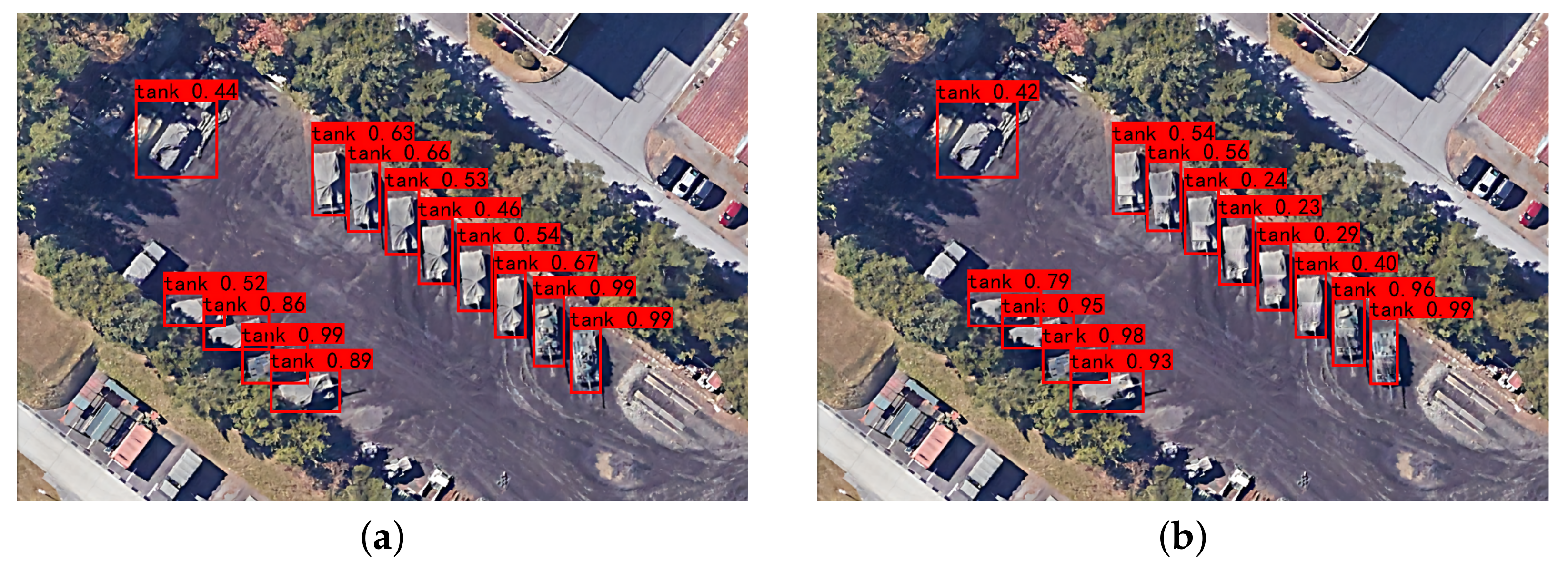
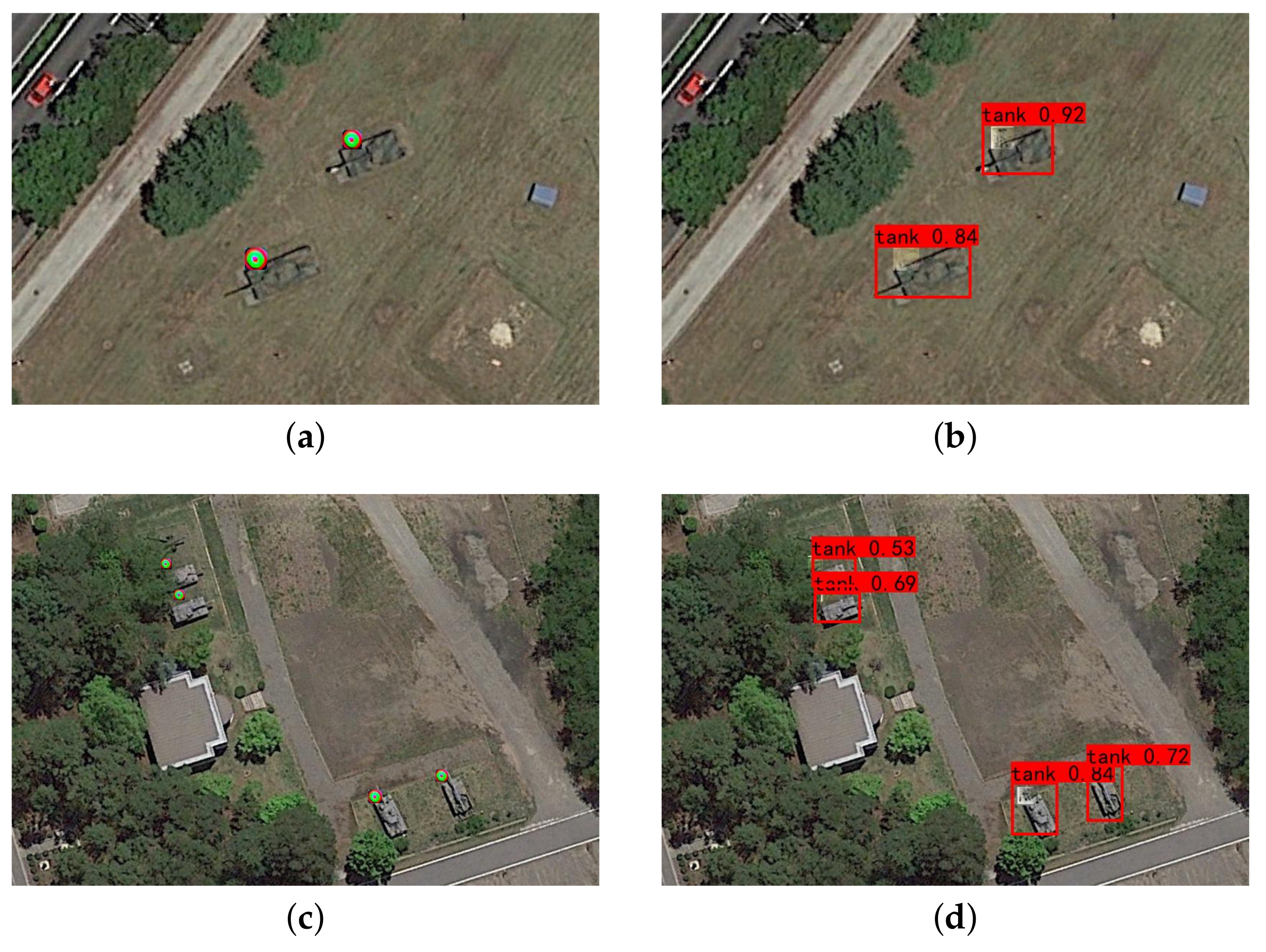
5.2.4. Defense Performance

We evaluate the performance of our algorithm on the YOLOv3 [49] and YOLOv4 [50] detectors and test it with the tank dataset. We first train YOLOv3 and YOLOv4, in which YOLOv3 is trained for 200 epochs and YOLOv4 is trained for 100 epochs. The backbone networks are Darknet53 and CSPDarknet53, respectively. All training data sizes are fixed to 416 × 416 pixels. The detection performance of the trained model is shown in Table 1 and Table 2. We set the IoU threshold $\mathrm{IoU}=0.5$ for YOLOv3 and $\mathrm{IoU}=0.2$ for YOLOv4 in our experiments unless otherwise stated, we set object score threshold from 0.01 to 0.9 for testing, expressed as Conf1 to Conf90, this index is used because we are mainly defending against vanishing attacks, and the object score can represent the confidence of whether there is an object in the bounding box. Recall, Precision, F1 and AP indices are used to show the performance of our algorithm.

The performance indices with subscripts (adv) represent the performance of the model without defense under adversarial patch attacks. The performance indices without subscripts represent the performance of the defense model under adversarial patch attacks, and the subscript (nat) represents the detection performance of the detector on clean examples. We directly attach the adversarial patch to the detection target to attack the detector. The adversarial patch is a rectangular block with the same length and width, and its size is just enough to cover the top of the detection target.

The detector performance under different conditions is shown in Table 1 and Table 2:

Table 1. The detection performance of the YOLOv3 without our defense algorithm on clean images and the adversarial patch attack, and the detection performance of the YOLOv3 with our defense algorithm under the adversarial patch attack.

Index	Conf1	Conf10	Conf20	Conf40	Conf60	Conf75	Conf90
Recall(nat)	76.87	76.87	76.87	76.87	69.86	56.54	32.72
Recall(adv)	0.00	0.00	0.00	0.00	0.00	0.00	0.00
Recall	75.70(↓1.17)	75.70(↓1.17)	75.70(↓1.17)	75.70(↓1.17)	67.99(↓1.87)	50.23(↓6.31)	26.64(↓6.08)
Precision(nat)	91.64	91.64	91.64	91.64	93.44	96.80	98.59
Precision(adv)	0.00	0.00	0.00	0.00	0.00	0.00	0.00
Precision	90.00(↓1.64)	90.00(↓1.64)	90.00(↓1.64)	90.00(↓1.64)	93.57(↓0.13)	96.41(↓0.39)	98.28(↓0.31)
F1(nat)	0.84	0.84	0.84	0.84	0.80	0.71	0.49
F1(adv)	0.00	0.00	0.00	0.00	0.00	0.00	0.00
F1	0.82(↓0.02)	0.82(↓0.02)	0.82(↓0.02)	0.82(↓0.02)	0.79(↓0.1)	0.66(↓0.05)	0.42(↓0.07)
AP(nat)	92.40	90.36	87.03	78.65	68.59	55.93	32.67
AP(adv)	0.01	0.00	0.00	0.00	0.00	0.00	0.00
AP	91.47(↓0.93)	89.30(↓1.06)	86.08(↓0.95)	78.87(↑0.22)	66.48(↓2.11)	52.52(↓3.41)	26.39(↓6.28)

Table 1. The detection performance of the YOLOv3 without our defense algorithm on clean images and the adversarial patch attack, and the detection performance of the YOLOv3 with our defense algorithm under the adversarial patch attack.

Index	Conf1	Conf10	Conf20	Conf40	Conf60	Conf75	Conf90
Recall(nat)	76.87	76.87	76.87	76.87	69.86	56.54	32.72
Recall(adv)	0.00	0.00	0.00	0.00	0.00	0.00	0.00
Recall	75.70(↓1.17)	75.70(↓1.17)	75.70(↓1.17)	75.70(↓1.17)	67.99(↓1.87)	50.23(↓6.31)	26.64(↓6.08)
Precision(nat)	91.64	91.64	91.64	91.64	93.44	96.80	98.59
Precision(adv)	0.00	0.00	0.00	0.00	0.00	0.00	0.00
Precision	90.00(↓1.64)	90.00(↓1.64)	90.00(↓1.64)	90.00(↓1.64)	93.57(↓0.13)	96.41(↓0.39)	98.28(↓0.31)
F1(nat)	0.84	0.84	0.84	0.84	0.80	0.71	0.49
F1(adv)	0.00	0.00	0.00	0.00	0.00	0.00	0.00
F1	0.82(↓0.02)	0.82(↓0.02)	0.82(↓0.02)	0.82(↓0.02)	0.79(↓0.1)	0.66(↓0.05)	0.42(↓0.07)
AP(nat)	92.40	90.36	87.03	78.65	68.59	55.93	32.67
AP(adv)	0.01	0.00	0.00	0.00	0.00	0.00	0.00
AP	91.47(↓0.93)	89.30(↓1.06)	86.08(↓0.95)	78.87(↑0.22)	66.48(↓2.11)	52.52(↓3.41)	26.39(↓6.28)

Table 2. The detection performance of the YOLOv4 without our defense algorithm on clean images and the adversarial patch attack, and the detection performance of the YOLOv4 with our defense algorithm under the adversarial patch attack.

Index	Conf1	Conf10	Conf20	Conf40	Conf60	Conf75	Conf90
Recall(nat)	98.13	98.13	98.13	98.13	98.13	97.66	96.26
Recall(adv)	0.00	0.00	0.00	0.00	0.00	0.00	0.00
Recall	96.26(↓1.87)	96.26(↓1.87)	96.26(↓1.87)	96.26(↓1.87)	96.03(↓2.10)	94.84(↓2.82)	92.76(↓3.50)
Precision(nat)	76.64	76.64	76.64	76.64	81.40	86.72	93.64
Precision(adv)	0.00	0.00	0.00	0.00	0.00	0.00	0.00
Precision	79.23(↑2.59)	79.23(↑2.59)	79.23(↑2.59)	79.23(↑2.59)	81.55(↑0.15)	85.00(↓1.72)	93.19(↓0.45)
F1(nat)	0.86	0.86	0.86	0.86	0.89	0.92	0.95
F1(adv)	0.00	0.00	0.00	0.00	0.00	0.00	0.00
F1	0.87(↑0.01)	0.87(↑0.01)	0.87(↑0.01)	0.87(↑0.01)	0.88(↓0.01)	0.90(↓0.02)	0.93(↓0.02)
AP(nat)	98.09	98.09	98.09	97.77	97.59	97.19	95.91
AP(adv)	0.11	0.00	0.00	0.00	0.00	0.00	0.00
AP	97.27(↓0.82)	96.84(↓1.25)	96.68(↓1.41)	95.79(↓1.98)	95.42(↓2.17)	94.84(↓2.35)	92.51(↓3.40)

Table 2. The detection performance of the YOLOv4 without our defense algorithm on clean images and the adversarial patch attack, and the detection performance of the YOLOv4 with our defense algorithm under the adversarial patch attack.

Index	Conf1	Conf10	Conf20	Conf40	Conf60	Conf75	Conf90
Recall(nat)	98.13	98.13	98.13	98.13	98.13	97.66	96.26
Recall(adv)	0.00	0.00	0.00	0.00	0.00	0.00	0.00
Recall	96.26(↓1.87)	96.26(↓1.87)	96.26(↓1.87)	96.26(↓1.87)	96.03(↓2.10)	94.84(↓2.82)	92.76(↓3.50)
Precision(nat)	76.64	76.64	76.64	76.64	81.40	86.72	93.64
Precision(adv)	0.00	0.00	0.00	0.00	0.00	0.00	0.00
Precision	79.23(↑2.59)	79.23(↑2.59)	79.23(↑2.59)	79.23(↑2.59)	81.55(↑0.15)	85.00(↓1.72)	93.19(↓0.45)
F1(nat)	0.86	0.86	0.86	0.86	0.89	0.92	0.95
F1(adv)	0.00	0.00	0.00	0.00	0.00	0.00	0.00
F1	0.87(↑0.01)	0.87(↑0.01)	0.87(↑0.01)	0.87(↑0.01)	0.88(↓0.01)	0.90(↓0.02)	0.93(↓0.02)
AP(nat)	98.09	98.09	98.09	97.77	97.59	97.19	95.91
AP(adv)	0.11	0.00	0.00	0.00	0.00	0.00	0.00
AP	97.27(↓0.82)	96.84(↓1.25)	96.68(↓1.41)	95.79(↓1.98)	95.42(↓2.17)	94.84(↓2.35)	92.51(↓3.40)

The F1 index in Table 1 and Table 2 represents the harmonic mean of Recall and Precision, it can take into account both the precision and the recall rate, which is a comprehensive evaluation index and requires that the overall high performance index must be established on the condition that both high precision and high recall rate are satisfied. F1 can be expressed as follows:

$$\begin{array}{c}\hfill \mathrm{F}1=\frac{2\ast \mathrm{Precision}\ast \mathrm{Recall}}{\mathrm{Precision}+\mathrm{Recall}}\end{array}$$

(18)

Here we use the most aggressive adversarial patch. We will introduce and analyze the weak adversarial patch later. It can be seen from Table 1 and Table 2 that under the attack of the adversarial patch, both YOLOv3 and YOLOv4 detectors are very fragile and can hardly detect any target, which indicates that the vanishing attack is successfully implemented. Before being attacked by the adversarial patch, both the YOLOv3 and YOLOv4 detectors showed good detection performance, and our defense algorithm can make the detection performance approach the detection performance before being attacked by the adversarial patch. We mainly need to ensure that the detector can detect the target normally and ensure that the AP index does not drop as much as possible. From the recall index in Table 1 and Table 2, we can see that our algorithm first ensures that the model can detect the target as much as possible under adversarial patch attacks. Under the object score threshold of 0.01 to 0.6, the recall rates of YOLOv3 and YOLOv4 drop by approximately 1% and 2%, respectively, which are very close to the original performance. Thus, the ineffectiveness of the vanishing attack under our algorithm is guaranteed. For the precision index, after inserting our algorithm, the YOLOv3 and YOLOv4 detectors have almost no change after being attacked, and YOLOv4 has even a better precision after being attacked. As seen from the AP, our algorithm almost restores the detection performance of the model that was present before being attacked by the adversarial patch, and it can be seen from the F1 indicator that our algorithm meets the requirements of high precision and high recall at the same time.

We fixed the object score threshold to 0.5 and changed the IoU value to test the performance of our algorithm, as shown in

Table 3. The detection performance of the YOLOv3 without our defense algorithm on clean images, and the detection performance of the YOLOv3 with our defense algorithm under the adversarial patch attack.

Index	AP(average)	AP35	AP50	AP75	AP90
Recall(nat)	76.87	76.87	76.87	76.87	76.87
Recall	75.70(↓1.17)	75.70(↓1.17)	75.70(↓1.17)	75.70(↓1.17)	75.70(↓1.17)
Precision(nat)	71.64	90.98	89.60	59.44	46.55
Precision	72.31(↑0.67)	91.27(↑0.29)	88.77(↓0.83)	59.59(↑0.15)	49.62(↑0.07)
AP(nat)	69.85	75.44	75.92	67.00	61.04
AP	68.70(↓1.15)	74.16(↓1.28)	73.84(↓2.08)	65.71(↓1.29)	61.12(↑0.08)

.

The results in Table 3 are similar to those in Table 1 and Table 2, indicating that our algorithm can effectively defend against adversarial attacks under different IoU.

In addition, we also consider the case where the adversarial patch is not directly attached to the detection target but is next to the detection target, as shown in Figure 9 because it is also possible to attack the detector without directly attaching it to the detection target. Since there is no need to inpaint the detection target, this situation can simulate the position accuracy of the adversarial patch position method.

As seen from

Table 4. The detection performance of YOLOv3 without defense and after defense when the adversarial patch is next to the detection target.

Index	Conf1	Conf10	Conf20	Conf40	Conf60	Conf75	Conf90
Recall(adv)	0.70	0.70	0.70	0.70	0.70	0.47	0.00
Recall	68.69	68.69	68.69	68.69	58.88	42.99	20.56
Precision(adv)	17.65	17.65	17.65	17.65	25.00	33.33	0.00
Precision	88.55	88.55	88.55	88.55	92.31	96.34	97.78
AP(adv)	1.19	0.60	0.01	0.01	0.01	0.01	0.00
AP	87.86	83.94	80.04	70.49	57.36	42.28	20.45

, although the attacking ability of the adversarial patch is slightly reduced, the detector is still far from being able to effectively detect the target. Our algorithm effectively restores the detection ability of the detector. We find that with the help of our algorithm, the detector performance is almost the same when the adversarial patch is directly attached to the detection target or placed next to the detection target. Thus, we can draw two conclusions:

1.

Since adversarial patch is not directly attached to the detection target, the accuracy of the adversarial patch position method can be simulated, so the localization method has high localization accuracy. Therefore, it can also be seen that image inpainting and training data augmentation can almost restore the detection performance of the detector.

2.

When the adversarial patch is close to the detection target, some target features will be lost due to the pooling operation, so the detection performance in this case is not completely the same as the performance before the attack;

From the above analysis, we can see the advantages of our algorithm in the positioning accuracy of adversarial patches. Furthermore, the model robustness under the image inpainting and data augmentation methods is significantly improved.

5.3. Ablation Studies

5.3.1. Why Does the Mutual Elimination Operation in the Gradient Domain Work?

According to our observations, there are two classes of adversarial patches. One class contains considerable high-frequency noise, and this kind of patch mainly attacks the digital domain. The other class of adversarial patches contains strong color gamut information and can attack in the physical domain. The second class of adversarial patch is characterized by the mutation of color, which is embodied in the mutation of color transition between regions. This allows the adversarial patch to obtain a large amount of gradient information in the gradient domain, and the gradient information does not affect each other in the same region. As shown in Figure 2, the gradient of the image is obtained separately in the RGB channel, and there is substantial gradient information at the edge of the color transition. Because the position of the transition area is different, the gradient of the adversarial patch will not be eliminated during the mutual elimination operation. In contrast, the image gradient obtained in the RGB channel of the natural image is the same in the transition area. Thus, it is easy to eliminate the natural image area after the mutual elimination operation.

5.3.2. Improvement of Detection Robustness by Random Erasing Algorithm

We first show the improvement of the detection robustness of the data augmentation algorithm. As described in the previous section, we set the minimum to maximum value of the erasing region with respect to the bounding box region from 0.02 to 0.2, The Erasing area’s length to width or width to length ratio is 0.1 to 1, and the filled pixel value is 1. We change the probability of enabling the random erasing algorithm and its aspect ratio range to represent its impact on detection robustness We set to not enable random erasing or enable random erasing with a probability of 20%, 50%, and 90% for comparison. We use rl to represent the aspect ratio range of the random erasing area; for example, rl = 0.5 means that the range of the ratio of length to width or width to length is $[0.5,1/0.5]$.

The lower confidence limit in Figure 10 is equivalent to the object score threshold. From Figure 10, we find that there is a large gap between the detection performance of enabling random erasing and not enabling random erasing. This is because the detector learns the situation of strong feature occlusion during training, and the detection robustness will be stronger in the face of weak feature occlusion. When the probability of random erasing is 20% and 90%, the performance of the detector is almost the same because an excessively low activation probability makes the model unable to effectively learn the example features when strong feature occlusion occurs, and an excessively high activation probability makes the model unable to effectively learn the overall effective features of the example. When the activation probability is 50%, the model can effectively balance the example features of feature occlusion and the overall effective features of the examples and thus stronger model robustness can be obtained. It is obvious from Figure 10 that the closer the area aspect ratio of random erasing is to 1, the better the detection performance. This is mainly because the shape of the adversarial patch is also a square with equal length and width. This shows that in the face of adversarial patches of different shapes, different rl values need to be selected to train the model.

5.3.3. Defense against Weakly Saliency Adversarial Patch

In addition, we also study weakly saliency adversarial examples, i.e., adversarial patch with visual concealment. As shown in Figure 8b, this kind of adversarial patch is more concealed, but it is also aggressive. Hence this adversarial patch can test the performance of our algorithm. To reduce the gradient of the adversarial patch, we process the adversarial patch with a Gaussian blur with a radius of 1, 2, 4 and 8 pixels to simulate the adversarial patch existing in the real environment, thus making the adversarial patch more difficult to locate. As shown in Figure 11, the attack and defense of weakly saliency adversarial patch, in order to demonstrate the attack ability of weakly saliency adversarial patch, we set the IoU threshold as low as possible to show the detection results of the detector under adversarial attack, Figure 7 is the same.

It can be seen from

Table 5. Model defense performance after processing adversarial patch with different Gaussian blur radii. Attack means that the defense algorithm is not used, and Robust means that the defense algorithm is used.

Blur Pixel Radius	Conf1		Conf20		Conf60		Conf90
	Attack	Robust	Attack	Robust	Attack	Robust	Attack	Robust
1(Recall)	15.42	69.63	15.42	69.63	10.28	60.28	1.87	20.09
1(AP)	52.09	89.75	24.49	82.38	9.60	59.27	1.87	20.09
2(Recall)	17.52	73.60	17.52	73.60	12.38	67.76	2.57	23.83
2(AP)	54.99	90.52	27.04	83.92	11.69	66.71	2.57	23.83
4(Recall)	18.22	73.83	18.22	73.83	14.02	66.12	2.80	27.10
4(AP)	57.89	90.72	29.53	84.37	13.29	65.00	2.80	27.09
8(Recall)	21.50	70.33	21.50	70.33	17.99	64.49	4.21	25.23
8(AP)	63.84	88.53	37.24	82.46	17.09	63.12	4.21	25.18

that the attack ability of the weakly saliency adversarial patch after Gaussian blurring is slightly weaker, but it is still aggressive and can effectively threaten the detector. With the increase in the blur radius, the aggressiveness decreases. Our algorithm significantly improves the robustness of detection, and the performance after defense is greatly improved. In the case of insignificant gradient information, our algorithm can effectively locate and inpaint weakly saliency adversarial patches. This shows that our algorithm can still guarantee the effectiveness of the algorithm under weak gradient information. Our algorithm achieves the best performance when the blur radius is 2 and 4 because a blur radius that is too large will lead to a sharp drop in gradient information, while a blur radius that is too small will cause the gradient information to be mainly concentrated in the central region, that is, the nongray area, so that the noncentral area cannot be completely inpainted.

5.3.4. Influence of Adversarial Patch Size on Image Inpainting and Adversarial Patch Positioning

The attacking ability of different sized adversarial patches is also different; the smaller the adversarial patch is, the weaker the attack ability, and vice versa, but the larger adversarial patch implies it is more obvious and hence it is easier to detect. For larger adversarial patches, it is more difficult to inpaint the region. For a small adversarial patch, although the difficulty of region inpainting decreases, the difficulty of locating the position increases. We use 10%, 30%, and 40% of the maximum width and height of the detection target to generate an adversarial patch with the same length and width for analysis. The adversarial patches of different sizes are shown in Figure 12. The adversarial patch size in the previous experiments is approximately 20% of the maximum width and height of the detection target.

It can be clearly seen from Figure 13 that a larger adversarial patch results in more performance degradation because the image inpainting algorithm cannot obtain effective texture and semantic information of the detection target, and the contextual attention module is almost ineffective. However, larger adversarial patches are easily eliminated by detection algorithms, while for small adversarial patches, their concealment ability is very strong and they are difficult to detect. Although their aggressiveness is not as high as that of weakly saliency adversarial patches, it is still threatening, and our algorithm can still perform effectively and restore the robustness of the detector under the attack of small adversarial patches. Figure 13 shows that as the area of the adversarial patch decreases, the performance of the detector is closer to the performance before being attacked by the adversarial patch. This indicates that our algorithm has good detection performance and robustness for adversarial patches of different sizes.

6. Conclusions

In this paper, we study the problem of adversarial examples in remote sensing detection and propose an adversarial defense method using position, inpainting and data augmentation. We conduct a detailed study on the “vanishing attack” in the adversarial attack, first define the vanishing attack problem, and note the definition of the defense against the adversarial example. We propose an adversarial example localization method based on the characteristics of adversarial patches under remote sensing detection, which can effectively locate adversarial patches under remote sensing detection, including weakly salient adversarial patches and adversarial patches of different sizes. We use an image inpainting technology based on deep learning to inpaint the adversarial patch area, combined with the random erasing algorithm to greatly improve the detection accuracy. Using our algorithm one can almost restore the performance of the detector before it was attacked. The experimental results show that our algorithm has strong robustness in various fields of remote sensing detection. This paper is reports the first research on the defense against adversarial attack under remote sensing detection. It provides a possible solution for the defense against adversarial examples. In future work, we hope to use an effective adversarial training method to improve the robust performance of the model itself based on the characteristics of the model thereby making it more robust in the face of adversarial attacks.

References

1. Van Etten, A. You only look twice: Rapid multi-scale object detection in satellite imagery. arXiv 2018, arXiv:1805.09512. [Google Scholar]
2. Guo, W.; Yang, W.; Zhang, H.; Hua, G. Geospatial object detection in high resolution satellite images based on multi-scale convolutional neural network. Remote Sens. 2018, 10, 131. [Google Scholar] [CrossRef] [Green Version]
3. Chen, X.; Xiang, S.; Liu, C.L.; Pan, C.H. Vehicle detection in satellite images by hybrid deep convolutional neural networks. IEEE Geosci. Remote Sens. Lett. 2014, 11, 1797–1801. [Google Scholar] [CrossRef]
4. Ji, H.; Gao, Z.; Mei, T.; Ramesh, B. Vehicle detection in remote sensing images leveraging on simultaneous super-resolution. IEEE Geosci. Remote Sens. Lett. 2019, 17, 676–680. [Google Scholar] [CrossRef]
5. Shermeyer, J.; Van Etten, A. The effects of super-resolution on object detection performance in satellite imagery. In Proceedings of the IEEE/CVF Conference on Computer Vision and Pattern Recognition Workshops, Long Beach, CA, USA, 15–20 June 2019. [Google Scholar]
6. Kim, J.; Cho, J. RGDiNet: Efficient Onboard Object Detection with Faster R-CNN for Air-to-Ground Surveillance. Sensors 2021, 21, 1677. [Google Scholar] [CrossRef]
7. Szegedy, C.; Zaremba, W.; Sutskever, I.; Bruna, J.; Erhan, D.; Goodfellow, I.; Fergus, R. Intriguing properties of neural networks. arXiv 2013, arXiv:1312.6199. [Google Scholar]
8. Goodfellow, I.J.; Shlens, J.; Szegedy, C. Explaining and harnessing adversarial examples. arXiv 2014, arXiv:1412.6572. [Google Scholar]
9. Tramèr, F.; Papernot, N.; Goodfellow, I.; Boneh, D.; McDaniel, P. The space of transferable adversarial examples. arXiv 2017, arXiv:1704.03453. [Google Scholar]
10. Su, J.; Vargas, D.V.; Sakurai, K. One pixel attack for fooling deep neural networks. IEEE Trans. Evol. Comput. 2019, 23, 828–841. [Google Scholar] [CrossRef] [Green Version]
11. Madry, A.; Makelov, A.; Schmidt, L.; Tsipras, D.; Vladu, A. Towards deep learning models resistant to adversarial attacks. arXiv 2017, arXiv:1706.06083. [Google Scholar]
12. Carlini, N.; Wagner, D. Towards evaluating the robustness of neural networks. In Proceedings of the 2017 IEEE Symposium on Security and Privacy (sp), San Jose, CA, USA, 22–26 May 2017; pp. 39–57. [Google Scholar]
13. Athalye, A.; Engstrom, L.; Ilyas, A.; Kwok, K. Synthesizing robust adversarial examples. In Proceedings of the International Conference on Machine Learning, PMLR, Stockholm, Sweden, 10–15 July 2018; pp. 284–293. [Google Scholar]
14. Brown, T.B.; Mané, D.; Roy, A.; Abadi, M.; Gilmer, J. Adversarial patch. arXiv 2017, arXiv:1712.09665. [Google Scholar]
15. Liu, X.; Yang, H.; Liu, Z.; Song, L.; Li, H.; Chen, Y. Dpatch: An adversarial patch attack on object detectors. arXiv 2018, arXiv:1806.02299. [Google Scholar]
16. Den Hollander, R.; Adhikari, A.; Tolios, I.; van Bekkum, M.; Bal, A.; Hendriks, S.; Kruithof, M.; Gross, D.; Jansen, N.; Perez, G.; et al. Adversarial patch camouflage against aerial detection. In Proceedings of the Artificial Intelligence and Machine Learning in Defense Applications II, Online, 21–25 September 2020; Volume 11543, p. 115430F. [Google Scholar]
17. Duan, R.; Mao, X.; Qin, A.K.; Chen, Y.; Ye, S.; He, Y.; Yang, Y. Adversarial laser beam: Effective physical-world attack to DNNs in a blink. In Proceedings of the IEEE/CVF Conference on Computer Vision and Pattern Recognition, Nashville, TN, USA, 20–25 June 2021; pp. 16062–16071. [Google Scholar]
18. Kaziakhmedov, E.; Kireev, K.; Melnikov, G.; Pautov, M.; Petiushko, A. Real-world attack on MTCNN face detection system. In Proceedings of the 2019 International Multi-Conference on Engineering, Computer and Information Sciences (SIBIRCON), Academpark, Russia, 21–22 October 2019; pp. 0422–0427. [Google Scholar]
19. Wu, Z.; Lim, S.N.; Davis, L.S.; Goldstein, T. Making an invisibility cloak: Real world adversarial attacks on object detectors. In Proceedings of the European Conference on Computer Vision, Glasgow, UK, 23–28 August 2020; pp. 1–17. [Google Scholar]
20. Huang, L.; Gao, C.; Zhou, Y.; Xie, C.; Yuille, A.L.; Zou, C.; Liu, N. Universal physical camouflage attacks on object detectors. In Proceedings of the IEEE/CVF Conference on Computer Vision and Pattern Recognition, Seattle, WA, USA, 13–19 June 2020; pp. 720–729. [Google Scholar]
21. Wang, J.; Liu, A.; Yin, Z.; Liu, S.; Tang, S.; Liu, X. Dual attention suppression attack: Generate adversarial camouflage in physical world. In Proceedings of the IEEE/CVF Conference on Computer Vision and Pattern Recognition, Nashville, TN, USA, 20–25 June 2021; pp. 8565–8574. [Google Scholar]
22. Thys, S.; Van Ranst, W.; Goedemé, T. Fooling automated surveillance cameras: Adversarial patches to attack person detection. In Proceedings of the IEEE/CVF Conference on Computer Vision and Pattern Recognition Workshops, Long Beach, CA, USA, 16–17 June 2019. [Google Scholar]
23. Hoory, S.; Shapira, T.; Shabtai, A.; Elovici, Y. Dynamic adversarial patch for evading object detection models. arXiv 2020, arXiv:2010.13070. [Google Scholar]
24. Chen, S.T.; Cornelius, C.; Martin, J.; Chau, D.H.P. Shapeshifter: Robust physical adversarial attack on faster r-cnn object detector. In Proceedings of the Joint European Conference on Machine Learning and Knowledge Discovery in Databases, Dublin, Ireland, 10–14 September 2018; pp. 52–68. [Google Scholar]
25. Dziugaite, G.K.; Ghahramani, Z.; Roy, D.M. A study of the effect of jpg compression on adversarial images. arXiv 2016, arXiv:1608.00853. [Google Scholar]
26. Das, N.; Shanbhogue, M.; Chen, S.T.; Hohman, F.; Chen, L.; Kounavis, M.E.; Chau, D.H. Keeping the bad guys out: Protecting and vaccinating deep learning with jpeg compression. arXiv 2017, arXiv:1705.02900. [Google Scholar]
27. Liao, F.; Liang, M.; Dong, Y.; Pang, T.; Hu, X.; Zhu, J. Defense against adversarial attacks using high-level representation guided denoiser. In Proceedings of the IEEE Conference on Computer Vision and Pattern Recognition, Salt Lake City, UT, USA, 18–23 June 2018; pp. 1778–1787. [Google Scholar]
28. Osadchy, M.; Hernandez-Castro, J.; Gibson, S.; Dunkelman, O.; Pérez-Cabo, D. No bot expects the DeepCAPTCHA! Introducing immutable adversarial examples, with applications to CAPTCHA generation. IEEE Trans. Inf. Forensics Secur. 2017, 12, 2640–2653. [Google Scholar] [CrossRef] [Green Version]
29. Papernot, N.; McDaniel, P.; Wu, X.; Jha, S.; Swami, A. Distillation as a defense to adversarial perturbations against deep neural networks. In Proceedings of the 2016 IEEE Symposium on Security and Privacy (SP), San Jose, CA, USA, 22–26 May 2016; pp. 582–597. [Google Scholar]
30. Hinton, G.; Vinyals, O.; Dean, J. Distilling the knowledge in a neural network. arXiv 2015, arXiv:1503.02531. [Google Scholar]
31. Song, Y.; Kim, T.; Nowozin, S.; Ermon, S.; Kushman, N. Pixeldefend: Leveraging generative models to understand and defend against adversarial examples. arXiv 2017, arXiv:1710.10766. [Google Scholar]
32. Samangouei, P.; Kabkab, M.; Chellappa, R. Defense-gan: Protecting classifiers against adversarial attacks using generative models. arXiv 2018, arXiv:1805.06605. [Google Scholar]
33. Lee, H.; Han, S.; Lee, J. Generative adversarial trainer: Defense to adversarial perturbations with gan. arXiv 2017, arXiv:1705.03387. [Google Scholar]
34. Athalye, A.; Carlini, N.; Wagner, D. Obfuscated gradients give a false sense of security: Circumventing defenses to adversarial examples. In Proceedings of the International Conference on Machine Learning, Stockholm, Sweden, 10–15 July 2018; pp. 274–283. [Google Scholar]
35. Zhang, H.; Wang, J. Towards adversarially robust object detection. In Proceedings of the IEEE/CVF International Conference on Computer Vision, Seoul, Korea, 27–28 October 2019; pp. 421–430. [Google Scholar]
36. Papernot, N.; McDaniel, P.; Jha, S.; Fredrikson, M.; Celik, Z.B.; Swami, A. The limitations of deep learning in adversarial settings. In Proceedings of the 2016 IEEE European Symposium on Security and Privacy (EuroS&P), Saarbruecken, Germany, 21–24 March 2016; pp. 372–387. [Google Scholar]
37. Moosavi-Dezfooli, S.M.; Fawzi, A.; Fawzi, O.; Frossard, P. Universal adversarial perturbations. In Proceedings of the IEEE Conference on Computer Vision and Pattern Recognition, Honolulu, HI, USA, 21–26 July 2017; pp. 1765–1773. [Google Scholar]
38. Lu, J.; Sibai, H.; Fabry, E.; Forsyth, D. No need to worry about adversarial examples in object detection in autonomous vehicles. arXiv 2017, arXiv:1707.03501. [Google Scholar]
39. Sharif, M.; Bhagavatula, S.; Bauer, L.; Reiter, M.K. Accessorize to a crime: Real and stealthy attacks on state-of-the-art face recognition. In Proceedings of the 2016 ACM Sigsac Conference on Computer and Communications Security, Vienna, Austria, 24–28 October 2016; pp. 1528–1540. [Google Scholar]
40. Du, A.; Chen, B.; Chin, T.J.; Law, Y.W.; Sasdelli, M.; Rajasegaran, R.; Campbell, D. Physical adversarial attacks on an aerial imagery object detector. In Proceedings of the IEEE/CVF Winter Conference on Applications of Computer Vision, Waikoloa, HI, USA, 4–8 January 2022; pp. 1796–1806. [Google Scholar]
41. Naseer, M.; Khan, S.; Porikli, F. Local gradients smoothing: Defense against localized adversarial attacks. In Proceedings of the 2019 IEEE Winter Conference on Applications of Computer Vision (WACV), Waikoloa Village, HI, USA, 7–11 January 2019; pp. 1300–1307. [Google Scholar]
42. Hayes, J. On visible adversarial perturbations & digital watermarking. In Proceedings of the IEEE Conference on Computer Vision and Pattern Recognition Workshops, Salt Lake City, UT, USA, 18–22 June 2018; pp. 1597–1604. [Google Scholar]
43. Chiang, P.Y.; Ni, R.; Abdelkader, A.; Zhu, C.; Studer, C.; Goldstein, T. Certified defenses for adversarial patches. arXiv 2020, arXiv:2003.06693. [Google Scholar]
44. Xiang, C.; Bhagoji, A.N.; Sehwag, V.; Mittal, P. {PatchGuard}: A Provably Robust Defense against Adversarial Patches via Small Receptive Fields and Masking. In Proceedings of the 30th USENIX Security Symposium (USENIX Security 21), Virtual, 11–13 August 2021; pp. 2237–2254. [Google Scholar]
45. Bao, J.; Chen, J.; Ma, H.; Ma, H.; Yu, C.; Huang, Y. Improving Adversarial Robustness of Detector via Objectness Regularization. In Proceedings of the Chinese Conference on Pattern Recognition and Computer Vision (PRCV), Beijing, China, 29 October–1 November 2021; pp. 252–262. [Google Scholar]
46. Telea, A. An image inpainting technique based on the fast marching method. J. Graph. Tools 2004, 9, 23–34. [Google Scholar] [CrossRef]
47. Yu, J.; Lin, Z.; Yang, J.; Shen, X.; Lu, X.; Huang, T.S. Generative image inpainting with contextual attention. In Proceedings of the IEEE Conference on Computer Vision and Pattern Recognition, Salt Lake City, UT, USA, 18–23 June 2018; pp. 5505–5514. [Google Scholar]
48. Zhong, Z.; Zheng, L.; Kang, G.; Li, S.; Yang, Y. Random erasing data augmentation. In Proceedings of the AAAI Conference on Artificial Intelligence, New York, NY, USA, 7–12 February 2020; Volume 34, pp. 13001–13008. [Google Scholar]
49. Redmon, J.; Farhadi, A. YOLOv3: An incremental improvement. arXiv 2018, arXiv:1804.02767. [Google Scholar]
50. Bochkovskiy, A.; Wang, C.Y.; Liao, H.Y.M. YOLOv4: Optimal speed and accuracy of object detection. arXiv 2020, arXiv:2004.10934. [Google Scholar]
Figure 1. Conceptual illustration of our method. We use the localization algorithm to locate the adversarial patch and remove the located adversarial patch and then use image inpainting technology to inpaint the removed area. We propose using the random erasing data augmentation algorithm to expand the training dataset to enhance the weak occlusion robustness of the model. Through the above framework, the detection robustness of the model will be greatly improved.
Remotesensing 14 03559 g001
Figure 2. The original adversarial patch and its corresponding RGB channel image and gradient image: (a) original image; (b) blue channel; (c) green channel; (d) red channel; (e) gradient image. (f,g): the gradient image of the adversarial patch in the real environment.
Remotesensing 14 03559 g002
Figure 3. Adversarial patch positioning process. ( x l r i , y l r i ) are the coordinates of the upper left and lower right corners of the i-th adversarial patch.
Remotesensing 14 03559 g003
Figure 4. The detection result of the image under the YOLOv3 detector: (a) detection results after the adversarial patches are removed; (b) detection results of the original image.
Remotesensing 14 03559 g004
Figure 5. (ad) Inpainting the adversarial patch area using traditional algorithms. Although the colors are similar, almost all the semantic and texture information in the inpainted area is lost, which is fatal to the detector.
Remotesensing 14 03559 g005
Figure 6. Image inpainting algorithm structure.
Remotesensing 14 03559 g006
Figure 7. (a) detection result of YOLOv3 on clean images; (b) detection result of YOLOv3 after defending with our algorithm under adversarial patch attack.
Remotesensing 14 03559 g007
Figure 8. Different types of adversarial patches: (a) strong adversarial patch generated by YOLOv3; (b) weak adversarial patch generated by YOLOv3; (c) strong adversarial patch generated by YOLOv4.
Remotesensing 14 03559 g008
Figure 9. (a,c) place the adversarial patch next to the detection target; (b,d) use our algorithm to detect figure (a,c).
Remotesensing 14 03559 g009
Figure 10. (a,b) Recall and AP of the model under different Random Erasing enabled probabilities; (c,d) Recall and AP of model under different Random Erasing aspect ratio ranges.
Remotesensing 14 03559 g010
Figure 11. (a) detection results of adversarial patch using Gaussian blur with a radius of 1 pixel under YOLOv3; (b) the detection result of the (a) after our defense algorithm.
Remotesensing 14 03559 g011
Figure 12. Adversarial patch with a size of (a) 10%, (b) 30%, (c) 40% of the maximum length and width of the detection target.
Remotesensing 14 03559 g012
Figure 13. Recall and AP index of the model under different adversarial patch sizes; (a) Recall rate under different adversarial patch sizes; (b) AP under different adversarial patch sizes.
Remotesensing 14 03559 g013