Abstract
To achieve high-resolution and wide-swath (HRWS) imaging, a space-time waveform-encoding (STWE) spaceborne synthetic aperture radar (SAR) system is adopted. In rugged terrain, the beam-pointing mismatch problem will appear when the traditional digital beamforming (DBF) technique is used to separate the received echoes. This problem leads to decreasing the received echo’s gain, deteriorating the quality of the image product and making the interpretation of SAR image difficult. To address this problem, an advanced echo separation scheme for STWE spaceborne SAR based on the DBF and blind source separation (BSS) is put forward in this paper. In the scheme, the echoes are transmitted within the adjacent pulse repetition intervals to simulate multiple beams, and the scattered echoes are received by the sixteen-channel antennas in elevation simultaneously. In post-processing, a detailed flow is adopted. In the method, the DBF is firstly performed on received echoes. Due to the error caused by terrain undulation, the degree of echo separation is not enough. Then, the BSS is performed on the multiple echoes obtained after the DBF processing. Finally, the highly separated echo signal can be obtained. In this scheme, there is no need to perform the direction of arrival (DOA) estimation before the DBF processing, which saves valuable computing resources. In addition, to verify the proposed scheme, point target and distributed target simulations based on the 16-channel data of an elevation X-band DBF-SAR system are carried out. The results of point targets indicate that the residual echo caused by rough terrain can be reduced by more than 14 dB using the proposed scheme. The proposed scheme can be directly implemented into existing SAR systems; thus, it does not increase the complexity of the system design. The scheme has the potential to be applied to future spaceborne SAR missions.
1. Introduction
Synthetic aperture radar (SAR) is one of the most important imaging systems, since radar is independent of weather and environmental conditions [1,2,3]. High-resolution and wide-swath (HRWS) imaging have been pursued by numerous scholars in recent years. On the one hand, more precise information can be acquired through higher resolution. On the other hand, better global observation capability can be achieved through wider swath [4,5,6]. Due to the minimum antenna area constrain [7,8,9], it is hard to improve the resolution and widen the swath concurrently for the traditional SAR [10,11]. To realize HRWS imaging, a series of methods and techniques have been proposed.
In 1989, Currie et al. [12,13] proposed to transmit a wide radar beam and adopt multiple beams in elevation to receive the signals of different sub-swaths. However, this method will result in serious range ambiguity due to the intervals between sub-swaths. Callaghan et al. [14] put forward a four-array mode in 1999. In this mode, the digital beamforming (DBF) in elevation was adopted to suppress the range ambiguity, which means the proposed scheme can improve the swath without decreasing the azimuth resolution, but it leads to the imaging blind area, limiting the development of the future spaceborne SAR. In 2001, Suess et al. [15] presented the HRWS mode. In this mode, the small aperture antenna and multiple channels were adopted to illuminate broad scene and receive the echoes, respectively. In addition, the azimuth multi-channel reconstruction was performed to suppress the azimuth ambiguity, and the Scan-On-Receive (SCORE) technique was used in elevation to enhance the antenna gain and suppress the range ambiguity. Krieger et al. [16] proposed the innovative concept of multidimensional waveform encoding (MWE) for the spaceborne SAR in 2007. In this mode, the waveform of each complete transmitted signal consists of several sub-pulses, and these sub-pulses were coded into four dimensions: space domain, time domain, frequency domain, and code domain to achieve waveform diversity, thus alleviating the conflicting requirements of radar sensors for high resolution, frequent revisit, and wide coverage. Recently, Zhang et al. [17] proposed the echo separation scheme for multiple-input and multiple-output (MIMO) SAR based on the segmented phase code (SPC) waveforms. However, this scheme requires encoding the selected initial radar waveforms using the encoding phase, which increases the complexity of the system design.
In a space-time waveform encoding (STWE) SAR system, each waveform of transmitted signal is composed of N sub-pulses of linear frequency modulation signal with identical time-frequency structure. These sub-pulses are emitted sequentially along different range or azimuthal sub-beams to meet the different performance requirements of the spaceborne SAR system. This paper mainly focuses on the STWE SAR system in elevation. In the STWE SAR system, the sub-pulses of a complete waveform are transmitted continuously; therefore, the echoes of these sub-pulses inevitably overlap during the echo reception period. To obtain the robust system performance of STWE SAR, the problem of accurate separation of echoes must be solved [18]. The DBF technique is used to separate echoes in STWE SAR [19,20,21,22], but due to the inevitable variation of topographic height and residual channel errors, the viewpoint deviation between real and virtual targets will lead to pointing errors in the antenna pattern, which will result in the reduced echo gain and insufficient interference suppression [23,24]. The interference that is not fully suppressed can cause the severe range ambiguity in the SAR image, which means that the system performance will be significantly degraded. In addition, the antenna pattern is extremely steep near null, and the loss caused by the insufficient interference suppression will be even more severe, which is unacceptable in a practical engineering system [25,26]. In order to reap the potential benefits that waveform diversity can provide for spaceborne SAR, echoes from different sub-pulses constituting a complete transmit waveform should be fully separated at first. Therefore, the problem of reduced echo gain and insufficient interference suppression caused by the topographic undulation of the observation scene is one of the bottlenecks limiting the development of STWE SAR.
To address the problem of reduced echo gain and insufficient interference suppression caused by the topographic undulation of the observation scene, the adaptive digital beamforming (ADBF) has been proposed [27,28,29]. The pointing error of the received beam is due to the incorrect estimation of the direction of arrival (DOA) of the target echo. The process of ADBF is shown as follows: after the original signal received from each sub-aperture in the range dimension is amplified by low-noise amplification (LNA), down-conversion and analog-to-digital conversion (ADC), it is firstly processed by range compression, which compresses the energy originally dispersed in the time domain of the target to its corresponding range gate and aligns the range-compressed image points about the same target in different sub-apertures to the same position, and then, the joint processing of multi-apertures is performed one by one to estimate the spatial spectrum, such as the Capon algorithm [30,31], Beamformer algorithm [32] and Music algorithm [33,34].
The process of ADBF is extremely computationally demanding because of the need for processing range bin by range bin, limiting the possibility of real-time processing on the future spaceborne STWE SAR in elevation.
To solve the problem mentioned above, this paper applied the blind source separation (BSS) to STWE SAR and proposed an advanced echo separation scheme for the first time. BSS originated from the famous “cocktail party effect” problem, which refers to a processing of the blind signal separation of target signals from noise without a priori information, with the aim of separating each person’s voice from the mixed sound signals received by multiple sensors [35,36,37]. In recent years, some scholars have studied the “cocktail party effect” in the field of SAR. Pu et al. [38] proposed a novel shuffle GAN with an autoencoder separation method to separate the moving and stationary targets in SAR imagery. Compared with the robust principal component analysis, the proposed method has a better performance. Chang et al. [39] proposed an advanced scheme for range ambiguity suppression of spaceborne SAR based on BSS. In the proposed scheme, the echoes are transmitted within the adjacent pulse repetition intervals to simulate multiple beams, and the scattered echoes are received by the sixteen-channel antennas in the range dimension simultaneously. In post-processing, a detailed flow is adopted. In the method, the DBF is firstly performed on received echoes. Due to the error caused by terrain undulation, the degree of echo separation is not enough. Then, the BSS is performed on the multiple echoes obtained after the DBF processing. Finally, the highly separated echo signal can be extracted. In this scheme, there is no need to perform the DOA estimation before the DBF processing, which saves valuable computing resources. In addition, the proposed scheme can be directly applied to current SAR systems, which means it does not increase the complexity of the system design under the current SAR system conditions.
The contents of this paper are arranged as follows. The conventional echo separation scheme and the disadvantages associated with the conventional echo separation scheme are described in Section 2. In Section 3, we primarily analyze the model of the BSS and the proposed echo separation scheme. The block diagram of the system architecture is also given in this section. In Section 4, the proposed scheme is verified by using a point target simulation, and a distributed target simulation verifies its echo separation ability by imaging simulation experiments using the 16-channel data in the elevation X-band DBF-SAR system. In Section 5, the conclusion is presented.
2. Problem Formulation
In this section, the conventional echo separation scheme is described. In addition, the disadvantages associated with the conventional echo separation scheme are pointed out as well.
2.1. Conventional Echo Separation Scheme
To obtain the wide swath in elevation, it can be seen that part sub-apertures are used to transmit pulse, and a plurality of sub-apertures are used to receive signals, as shown in Figure 1. Figure 1 shows the geometric model of DBF imaging in elevation, where is the slant range of the target A. The transmitted signal can be expressed as
where represents the fast time, T is the pulse duration, represents the carrier frequency, and is the frequency modulation rate. It is assumed that the number of the elevation sub-apertures is N, the distance between the adjacent sub-aperture is d, and the reference channel is channel 1. The echo signal received by the reference channel can be described as
where is the two-way delay from point A to channel 1. Similarly, the echo signal received by the m th channel in elevation can be formulated as:
where is the delay between the echo returned from point A to channel 1 and channel m, and it is
where c is the speed of light, is the off-boresight angle of point A, and is the interval between channels. Taking (4) into (3) and simplifying it, it can be approximated that
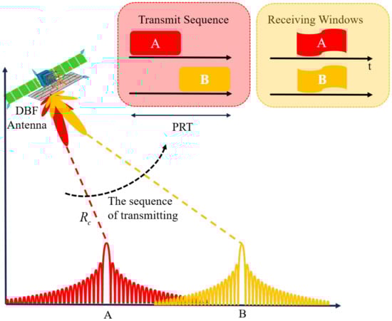
Figure 1.
The geometric model of DBF imaging in elevation.
In the data processing of the DBF in elevation, to realize the coherent accumulation of the signals of each channel, it is necessary to perform time-varying weighting processing on the signals received by the multiple channels in elevation, so that the center of the formed receiving beam can always point to the pulse center. For this reason, the weighting coefficient corresponding to the m th channel in elevation can be described as
To greatly increase the swath in elevation, the range multi-beam mode is adopted. The range multi-beam mode can be divided into two types: intra-pulse multi-beam and inter-pulse multi-beam. Inter-pulse multi-beam refers to transmitting multiple sub-beams in different pulse repetition intervals in the range to illuminate different sub-swaths. Intra-pulse multi-beam refers to the emission of multiple sub-beams within the same pulse repetition period to illuminate different sub-swaths. Compared with the inter-pulse multi-beam mode, the intra-pulse multi-beam mode can significantly reduce the pulse repetition frequency (PRF) of the SAR system, but at the same time, it will cause echo aliasing, which makes SAR image interpretation difficult and deteriorates the performance of the SAR system, so the echo separation based on intra-pulse multi-beam is an urgent problem to be solved. In order to solve the echo separation problem of intra-pulse multi-beam, the null-steering technique is proposed. The core of the null-steering technology is to generate a null in a specific direction of the antenna pattern during data processing, so that the null points to the interference signal, thereby suppressing the interference signal and improving the signal-to-noise ratio (SNR).
It is assumed that the number of sub-swaths in elevation is k th and DOA of each sub-swath is . The transmitted signal echo can be expressed as
where denotes the delay of the k th beam compared to the first transmitting beam. The echo signal of the m th receiving channel can be formulated as
where is the slant of the point A in k th sub-beam. If the above signals are represented in the form of vectors, the output signals of all receive apertures can be expressed as
In (9), , , , and
where indicates the distance between the phase center of the transmit channel and the n th receive channel.
The essence of echo separation is making echo signals from one sub-pluse with high gain and suppressing echoes from other sub-pluses. The above can be expressed as
where represent the two sub-swaths, respectively, is the weighting vector for extracting the received signals from the sub-pluse m, denotes the number of sub-apertures in elevation, and represent the steering vectors for echoes from the sub-pluse m and n, and represents the conjugate transpose.
For the beamforming described as (11) and (12), the problem of echo separation can be solved by using the linearly constrained minimum variance (LCMV) [40,41,42,43].
Define as
According to the LCMV, the weighting vector for separating the echo signals from the k th sub-pluse is
where is the column vector with the element being 1 and the remaining elements being 0, and represents the transpose.
2.2. Influence of Elevation Error on Conventional Echo Separation Scheme
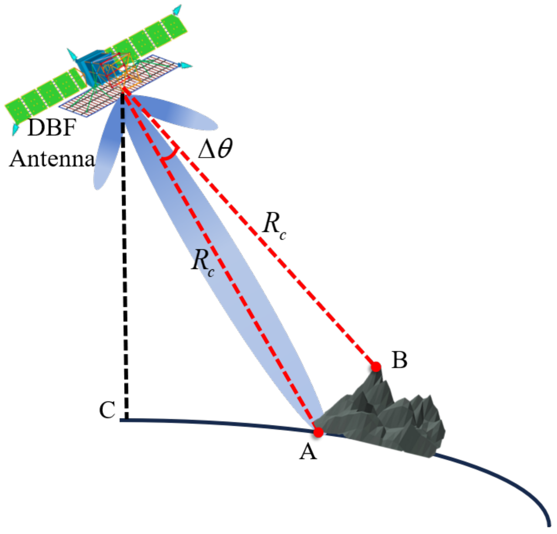
The DBF beamforming weighted vector discussed above is based on the premise that the Earth is a smooth ideal sphere. In the actual situation, the topography of Earth is more complex, with basins, hills and oceans. If the weighting vector is still calculated based on the ideal situation in the region with large topographic undulations, it will lead to errors in beam pointing, resulting in a loss of receive gain and deterioration of echo separation performance. Figure 2 shows a diagram of the beam pointing error. The real source position is point B at the top of the mountain, whose height is h, but the position calculated under the smooth ideal sphere model is point A at the bottom of the mountain. Based on the conventional pitch DBF technique, the source position will be deviated, resulting in the loss of the received gain of the echoes.
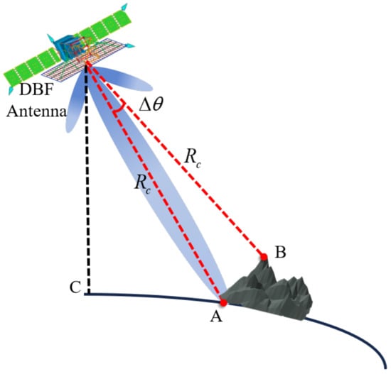
Figure 2.
The diagram of the beam pointing error. The target point is the point B at the top of the mountain and the wrong point is the point A at the bottom of the mountain.
As shown in Figure 2, the radius of Earth is and the height of the satellite orbit is . Then, under the smooth ideal sphere model, the viewpoint of the nadir at the wrong point A is
However, the viewpoint of nadir at the correct point B can be described as
The loss of the received echo’s gain due to the deviation of the view of nadir can be expressed as
where represents the height of the receiving antenna.
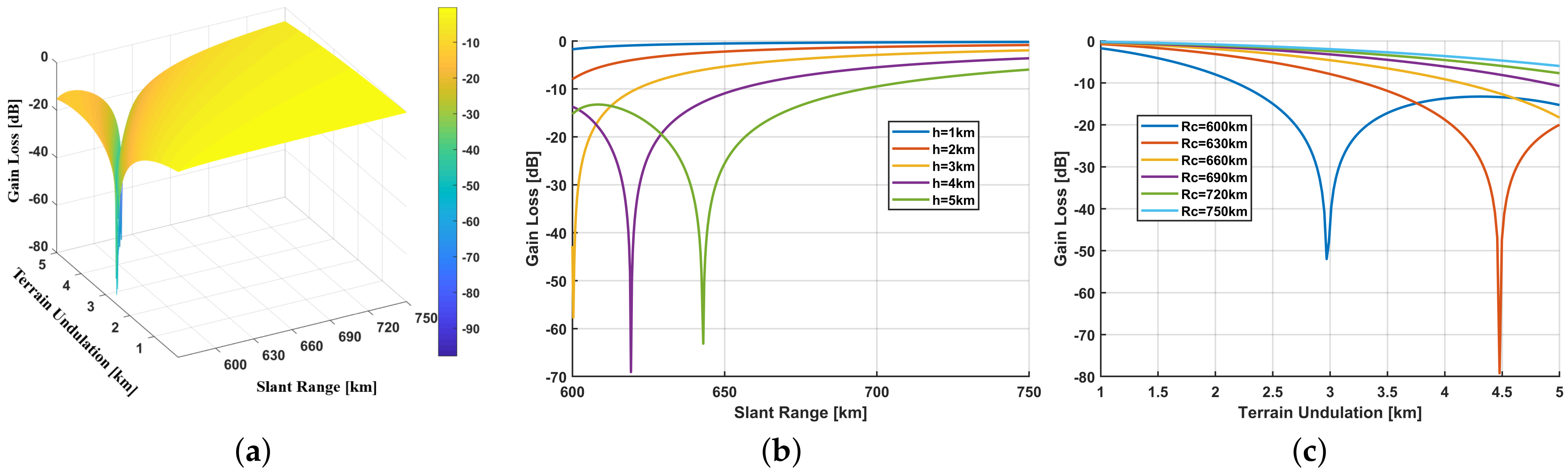
Based on the parameters of the spaceborne SAR system in Table 1, the relationship between the received gain loss and the slant range as well as the variation of the terrain undulation can be obtained as shown in Figure 3.

Table 1.
Simulation parameters.
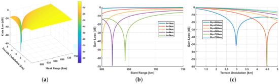
Figure 3.
The relationship between the received gain loss and the slant range as well as the variation of the terrain undulation. (a) 3D graph. (b) Gain Loss versus slant range. (c) Gain Loss versus terrain undulation.
Overall, under the condition of a certain slant range, the received gain loss increases with the height of the terrain undulation; when the height of the terrain undulation is certain, the received gain loss becomes smaller as the slant range increases. As can be seen in Figure 3, the antenna pattern is extremely steep near null, and the loss caused by insufficient interference suppression will be even more severe, which is unacceptable in a practical engineering system.
In addition, when the height of terrain undulation is greater than 3 km, the received gain loss can be greater than 3 dB, which can seriously deteriorate the image quality. For this reason, a series of schemes have been proposed to solve this problem. The core of these schemes is to estimate the exact DOA of the real target, and these schemes can be divided into two categories according to parametric and nonparametric, among which the main parametric algorithms are MUSIC and ESPIRIT [44], and the main nonparametric algorithms are Beamformer and Capon. Considering the robustness as well as portability of the algorithms, non-parametric algorithms are generally used in practice. These two algorithms require accurate estimation of DOA of the source at each range bin, and once there is a pointing error, it will result in the loss of echo gain, leading to the reduction of system performance and deterioration of product quality. These two algorithms are extremely computationally intensive because they require estimation processing for each range bin, making it difficult to perform real-time processing onboard. In the scheme proposed in this paper, DOA estimation is not required before DBF processing, thus saving valuable computing resources.
3. Echo Separation Scheme
Many difficult problems in the radar field are very similar to challenges in acoustics. Inspired by the “cocktail party effect” problem, this paper applies the combination of the DBF and BSS to STWE SAR echo separation for the first time to solve the problem that DBF is sensitive to the variation of topographic height. In this section, the proposed scheme based on the DBF and BSS is described in detail.
3.1. Blind Source Separation Model
Without considering time delay, it is assumed that there are K mutually independent source signals incident on M receiver units, and the mixed signal received by each receiver unit is a linear combination of the K source signals. The mixed signal model can be described as
where is the source signal vector, is the observed signal vector, and is an -dimensional unknown mixing matrix. The purpose of blind source separation is to calculate the separation matrix , which can be expressed as
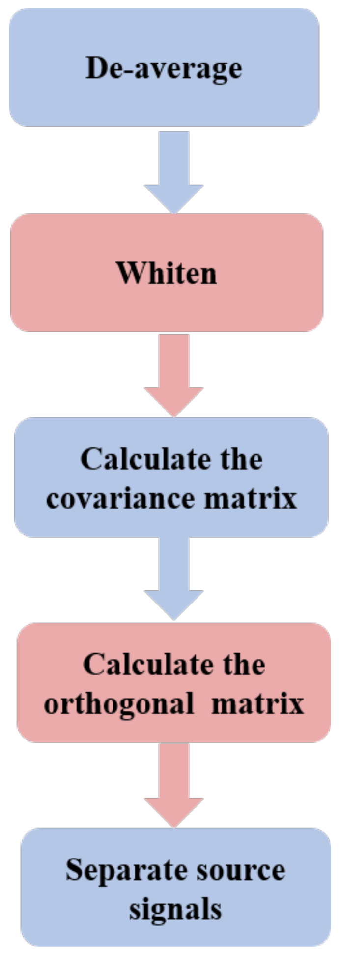
The processing of separating the mixed signal is as follows (Figure 4) [45]:
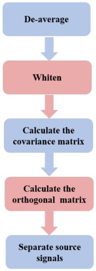
Figure 4.
Flowchat of the blind source separation.
- (1)
- De-average:
Subtract the mean of the signal from the observed signal values to make the observed signal a zero-mean vector.
- (2)
- Whiten:
Remove the second-order correlation of each observed signal.
- (3)
- Calculate the covariance matrix:
The delay covariance matrix of the source signal can be expressed as
where is the time delay amount. After whitening, can be expressed as
By choosing a set of different values such as , a series of delay covariance matrices can be obtained as
- (4)
- Calculate the orthogonal matrix:
Since the source signals are uncorrelated and the quantities in the matrix after whitening are orthogonally normalized to each other, the matrix is normalized orthogonal. Therefore, the optimal unitary matrix is found using and the optimal approximation algorithm, and thus, the whitened matrix is jointly diagonalized.
- (5)
- Separate source signals:
The optimal unitary matrix can be calculated, and the separation matrix can be expressed as:
After the above five steps, the separated echo signal can be obtained.
3.2. Proposed Scheme
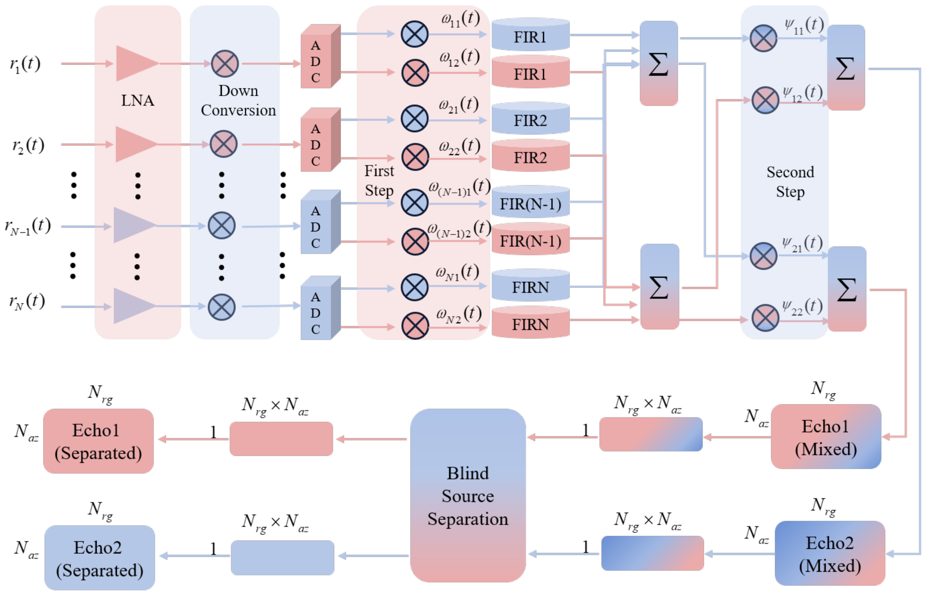
In this paper, an advanced STEW SAR echo separation scheme is proposed. As shown in Figure 5, the echo signals received by the multiple sub-apertures simultaneously need to be amplified, down-converted, and sampled first, and then, they undergo subsequent processing. Since the overlapping echoes come from different directions in elevation, it is possible to separate the mixed echoes by forming null-steering sub-beams simultaneously. Each sub-beam is steered in the time-varying direction of the echo, while a depth null is set in the time-varying direction of the interfering echo.
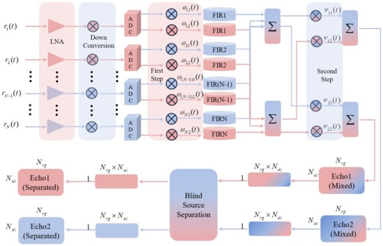
Figure 5.
Proposed echo separation scheme. The echo signals received by the multiple sub-apertures simultaneously need to be amplified, down-converted, and sampled first. represents the element in ; denotes the element of . The transfer function of the FIR filter for the k th sub-aperture is . LCMV is used to perform the first step of separation; after the LCMV processing, the BSS is performed.
As mentioned in Section 2, the LCMV is used to solve the weighting vector for separating the echo form the sub-swath. The the weighting vector can be expressed as (14). As shown in Figure 5, the LCMV can be divided into two steps:
- (1)
- Echoes received by all sub-apertures in elevation are weighted by two vectors denoted by rows of ;
- (2)
- The outputs of vetors are weighted by the corresopnding elements in and combined to extract the echo signals from the k th sub-pulse.
Based on the conventional LCMV beamformer, [25] proposed an advanced beamformer with FIR delay filters, as shown in Figure 5. The FIR delay filters are applied to relieve the influence of the extended pulse for the desired signal and the interfering signal. The transfer function of the FIR filter for the k th sub-aperture can be expressed as [25]
where is the carrier frequency of the system and is the range frequency rate.
The signal obtained after the LCMV processing can achieve partial separation. However, due to the undulating terrain, relying on LCMV only will result in the problem of insufficient separation, which will affect the subsequent product processing. Therefore, after the LCMV processing, the BSS processing is requried.
As shown in Figure 5, the application of BSS in echo separation of the STWE spaceborne SAR is shown as follows:
- (1)
- The echo signal matrix after the LCMV processing is a matrix of size , where , denote the number of azimuth and range sampling points, respectively. Then, the echo signal matrix is stretched into a row vector signal, and the mixed signal matrix is formed.
- (2)
- Apply BSS to the mixed signal matrix and process it: de-averaging, whitening, solving the unitary matrix and joint diagonalization, as shown in Section 3.
- (3)
- Restore the separated signals to signal matrices by rows.
The processing of BSS does not require prior knowledge, that is, terrain fluctuations will not deteriorate the performance of the separation. Therefore, the received echo signals obtained after LCMV-BSS joint processing are relatively pure echo signals, and subsequent operations such as imaging can be performed.
4. Simulation
In this section, a point target simulation and a distributed target simulation based on the data of the airborne 16-channel X-band DBF-SAR system are carried out to validate the performance of the proposed echo separation scheme.
4.1. Point Target Simulation
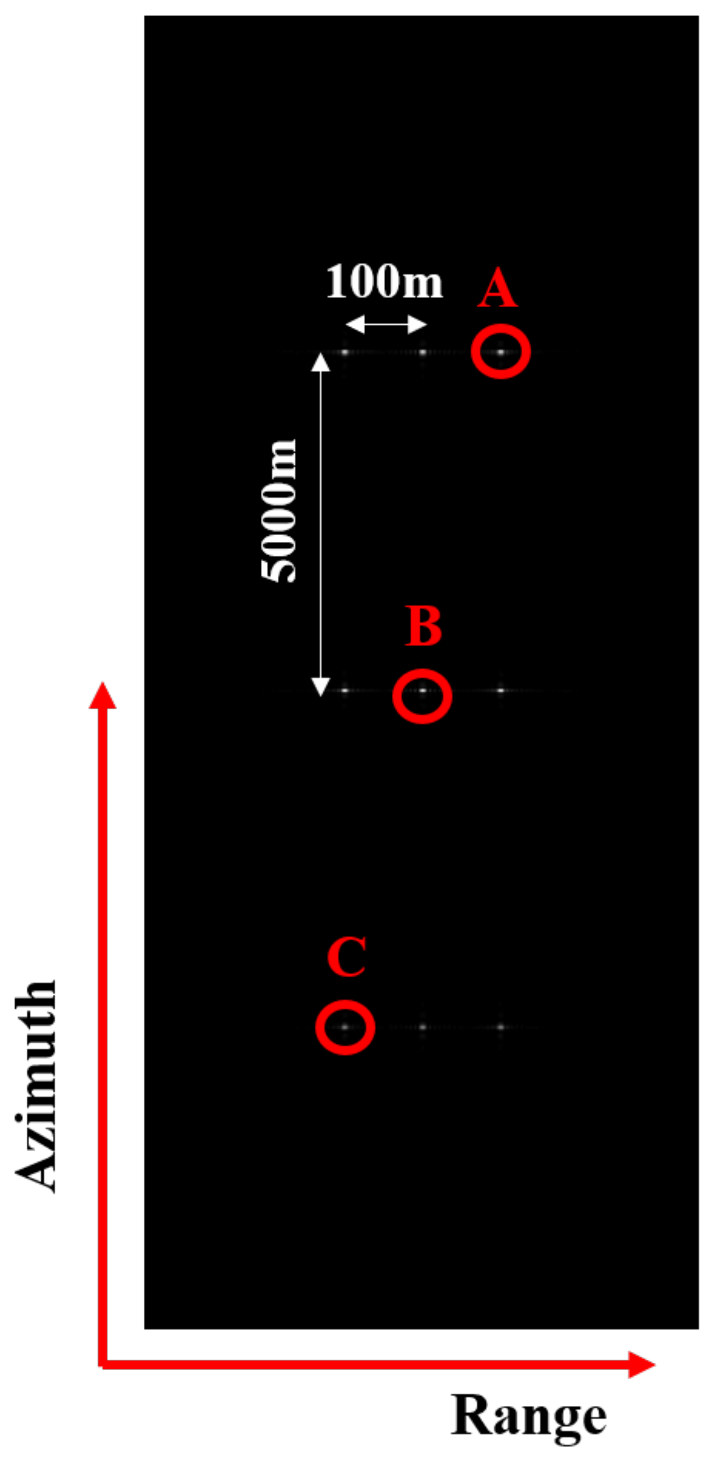
The simulation adopts an array of nine targets, laid out on a 200 × 10,000 m2 grid in ground range/azimuth, as shown in Figure 6, where the horizontal and vertical axes are the range and azimuth dimensions, respectively. In order to more intuitively see the influence of the residual signal on the main signal, the distribution in elevation is arranged more closely. Point B is the center of the scene (the reference point target), while points A and C are the farthest targets from point B. The point simulation parameters are shown in Table 2. The scene center slant range of sub-swath 1 is 631.7 km, while the scene center slant range of sub-swath 2 is 622.7 km. The angle error corresponding to the elevation error of 2.25 km is 0.48°. The diagram of point target simulations is shown in Figure 1. The echoes are transmitted within the adjacent PRIs to simulate multiple beams and the scattered echoes are received by the sixteen-channel antennas in elevation simultaneously.
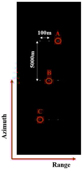
Figure 6.
Nine simulated point targets. Point B is the center of the scene (the reference point target), while points A and C are the farthest targets from point B.
Table 2.
The point simulation parameters.
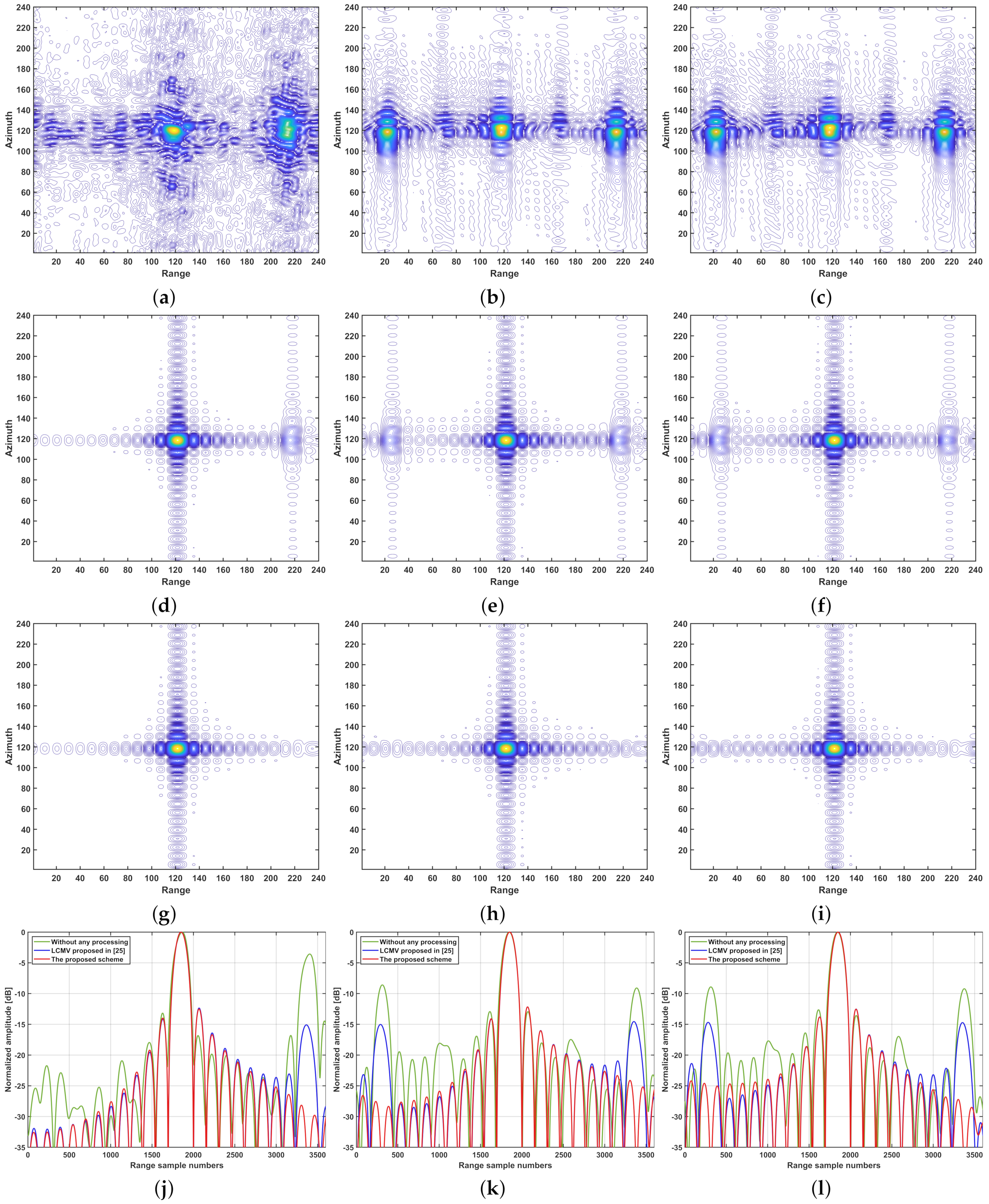
The simulated data are processed using the Chirp Scaling Algorithm (CSA) [46,47,48]. The echo imaging results of targets A, B, and C in sub-swath 1 without any processing are shown in Figure 7a–c respectively. To measure the impact of echo separation on imaging quality, some imaging evaluation indicators are calculated, such as the resolution, the peak sidelobe ratio (PSLR), and the integrated sidelobe ratio (ISLR). From Figure 7a–c and Table 3, it can be seen that LCMV processing was not performed in this experiment. Due to the superposition of echoes, the imaging quality was seriously deteriorated, resulting in the existence of false targets. Due to the existence of range ambiguity, the image quality deteriorated greatly. The mean of PSLR and ISLR in the range dimension is −7.02 dB and −3.71 dB. The mean of PSLR and ISLR in the azimuth dimension is −7.86 dB and −7.40 dB. All the indicators mentioned above are much higher than the theoretical values of −13.26 dB and −10.00 dB. Therefore, echo separation is an urgent problem to be solved in STWE SAR.
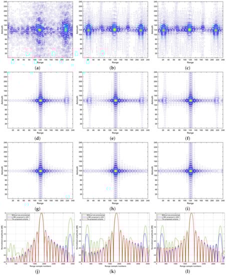
Figure 7.
Echo imaging results. (a) Point A in sub-swath 1 without any processing. (b) Point B in sub-swath 1 without any processing. (c) Point C in sub-swath 1 without any processing. (d) Point A in sub-swath 1 using the method proposed in [25]. (e) Point B in sub-swath 1 using the method proposed in [25]. (f) Point C in sub-swath 1 using the method proposed in [25]. (g) Point A in sub-swath 1 with the proposed scheme. (h) Point B in sub-swath 1 with the proposed scheme. (i) Point C in sub-swath 1 with the proposed scheme. (j) Range profile of Point A in sub-swath 1. (k) Azimuth profile of Point A in sub-swath 1. (l) Range profile of Point B in sub-swath 1. Green, blue and red represents the results without any prosessing, with LCMV proposed in [25] and with the proposed scheme, respectively.
Table 3.
Imaging evaluation indicators for the point targets without any processing.
The echo imaging results of targets A, B, and C in sub-swath 1 using the method proposed in [25] are shown in Figure 7d, e and f, respectively. The evaluation indicators of the point targets processed using LCMV proposed in [25] are shown in Table 4. From Figure 7d–f and Table 4, it can be seen that the image quality has been improved after LCMV processing compared with the results without any processing. Due to the existence of an elevation error of 2.25 km, there is a certain loss in the received echo gain, and the echoes may not be completely separated.
Table 4.
Imaging evaluation indicators for the point targets using the method proposed in [25].
There are ghost targets of −15.16 dB in Figure 7j, ghost targets of −15.02 dB and −14.55 dB in Figure 7k, and ghost targets of −14.68 dB and −14.59 dB in Figure 7l. These ghost targets cannot be ignored in practice, so it is unreliable to only rely on LCMV to separate echo signals.
The echo imaging results of targets A, B, and C in sub-swath 1 with LCMV-BSS joint processing are shown in Figure 7g, h and i respectively. The evaluation indicators of the point targets processed using LCMV-BSS are shown in Table 5. From Figure 7g–i and Table 5, it can be seen that indices improved considerable and reached their theoretically optimal values. Compared with the results obtained by LCMV processing only, the problem of a certain loss of the received echo gain caused by the elevation error of 2.25 km has been perfectly solved, and the echoes are well separated, which indicates that the proposed scheme is effective in the point target scenes.
Table 5.
Imaging evaluation indicators for the point targets with LCMV-BSS joint processing.
4.2. Distributed Target Simulation
Airborne SAR systems have been one step ahead of spaceborne SAR systems in technological development, and it can demonstrate new technologies and applications that are later implemented in spaceborne SAR missions. In the distributed target simulation, the data of the airborne 16-channel X-band DBF-SAR system is used. The used airborne DBF-SAR is developed by the Aerospace Information Research Institute, Chinese Academy of Sciences (AIRCAS) [17,19,22].
Considering the complexity of the airborne DBF-SAR switching different transmit beams in a PRT, this part adopts the data of inter-pulse multi-beams, and the pointing angle of two transmitting sub-beams A and B in elevation is 60° and 70°, respectively. Correspondingly, the obtained results correspond to sub-swaths A and B, respectively.
The main parameters of the airborne SAR system are shown in Table 6. To simulate the echo of multiple beams in the pulse, the received echo of sub-band A and the echo of sub-band B are superimposed.
Table 6.
The main parameters of the airborne SAR system.
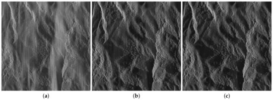
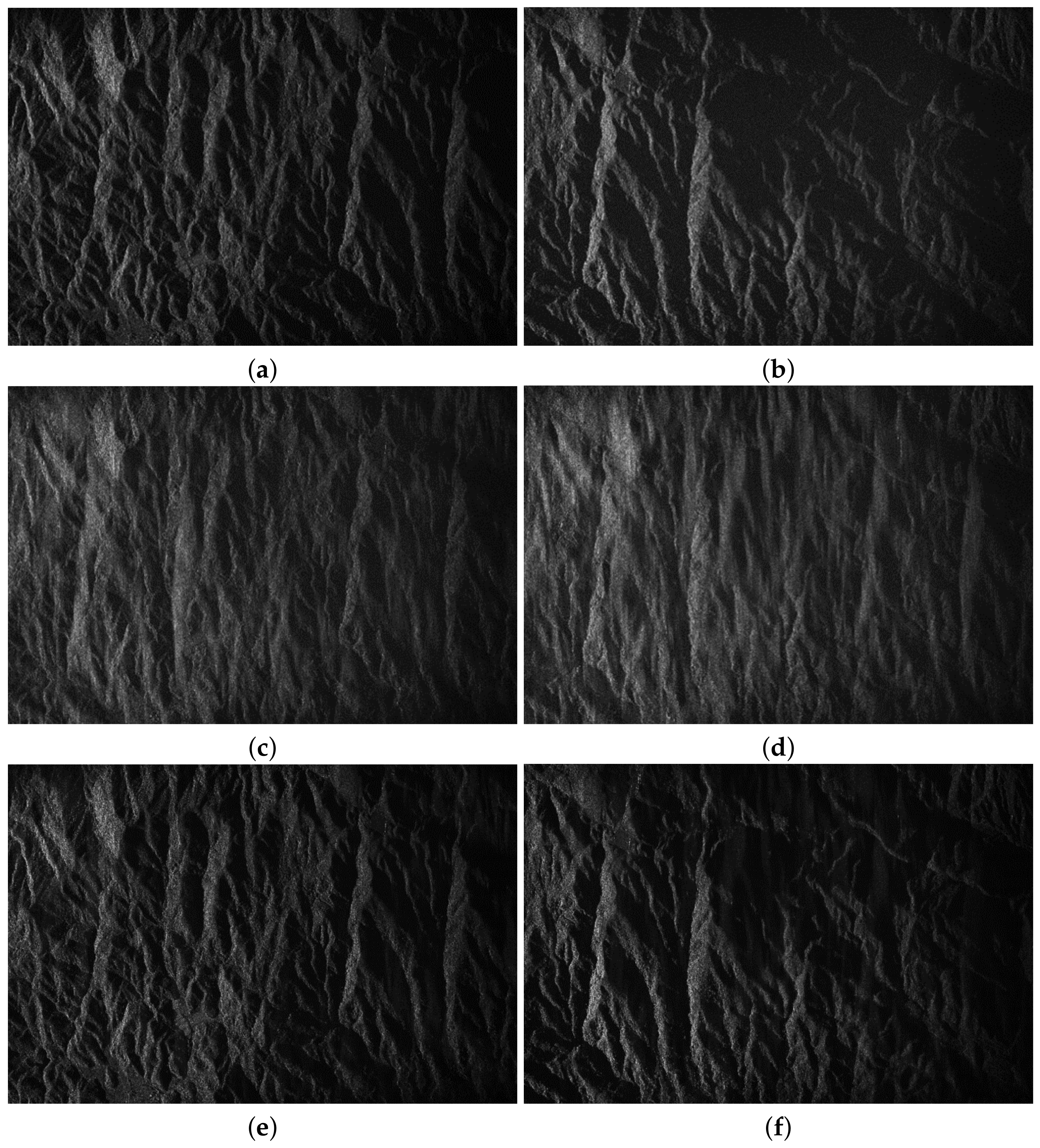
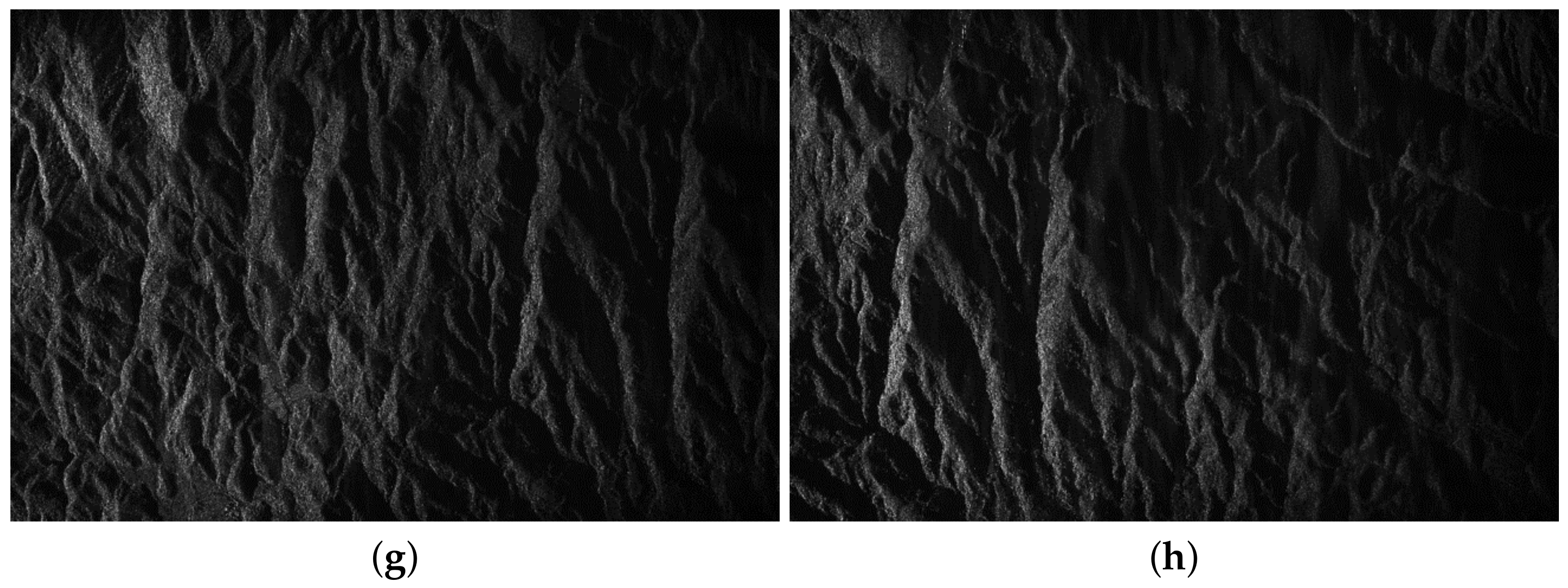
The imaging results are shown in Figure 8, where the horizontal vertical axes are the range and azimuth dimensions, respectively. Figure 8a,b are the original distributed scene imaging results of the sub-swath A and sub-swath B, respectively. To reflect the influence of terrain fluctuations on echo separation, the two selected areas are mountainous areas with large terrain fluctuations.

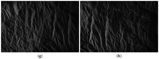
Figure 8.
Imaging results. (a) Original distributed scene imaging results of sub-swath A. (b) Original distributed scene imaging results of sub-swath B. (c) The simulated mixed echo of sub-swath A. (d) The simulated mixed echo of sub-swath B. (e) Distributed scene imaging results processed by LCMV proposed in [25] of sub-swath A. (f) Distributed scene imaging results processed by LCMV proposed in [25] of sub-swath B. (g) Distributed scene imaging results processed by LCMV-BSS of sub-swath A. (h) Distributed scene imaging results processed by LCMV-BSS of sub-swath B.
Figure 8c,d show the simulated mixed echo. Figure 8e,f are the echo imaging results obtained by LCMV proposed in [25]. Since the selected areas are all mountainous areas, the terrain fluctuation has a great influence on echo separation, so there are still residual echoes, which affects the image quality. Figure 8g,h are distributed scene imaging results obtained by LCMV-BSS joint processing.
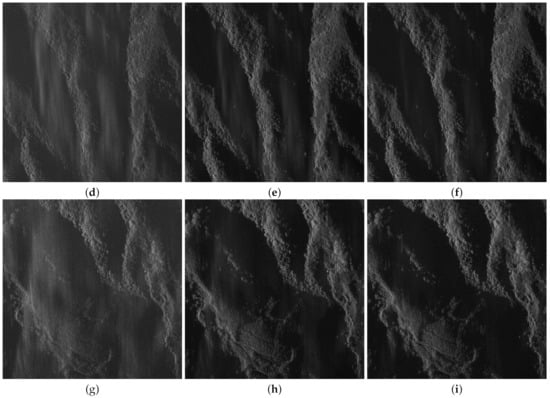
To see the difference between Figure 8e–h more clearly, Figure 9 is given. Figure 9 is a partial enlargement of the obtained images from Figure 8c–h. It can be seen from Figure 9 that the proposed LCMV-BSS scheme solves the problem of the loss of echo receiving gain caused by terrain fluctuation.
In order to quantitatively analyze the performance of the proposed scheme, we introduce two evaluation metrics, the peak-signal-to-noise ratio (PSNR) and the structural similarity index measure (SSIM) [49].
Given a reference image f and a test image g, both of size , the PSNR between f and g is defined by:
A higher PSNR value means the image quality is higher. The SSIM is used to measure the similarity between two images. The SSIM is defined as:
where
where is the luminance comparison function, and are the image’s mean luminance, is the contrast comparison function, and are the standard deviation, is the structure comparison function, and σfg is the covariance between f and g. The positive constants C1, C2 and C3 are used to avoid a null denominator.
The value of the SSIM index is in [0,1]. A value of 0 means no correlation between images, and 1 means that f = g.
Evaluation indicators for the distributed targets are shown in Table 7. It can be seen from Table 7 that the proposed scheme has a certain improvement compared with the conventional scheme in the two evaluation indicators of PSNR and SSIM, and it can effectively solve the problem of insufficient echo separation caused by terrain fluctuations.
Table 7.
Evaluation indicators for the distributed targets.
5. Conclusions
Echo separation is one of the main limitations for the future development of spaceborne SAR. Based on the domestic 16-channel airborne DBF-SAR system in elevation, an advanced echo separation scheme for STWE SAR based on the DBF and BSS is proposed in detail in this paper. This solution is designed to address the problem of reduced echo gain and insufficient interference suppression caused by the topographic undulation of the observation scene. In this paper, the results and corresponding analysis of the echo separation in the terrain relief area of the 16-channel airborne DBF-SAR system in elevation are presented for the first time.
In the proposed scheme, multiple sub-apertures are used for simultaneous reception. After the received echo signal is amplified, down-converted, and sampled, the LCMV is used to perform the first step of separation. Due to terrain fluctuations, the degree of separation is not enough. The residual echoes will affect the subsequent processing. Therefore, after the LCMV processing, the BSS is performed. The processing of BSS does not require prior knowledge, that is, terrain fluctuations will not deteriorate the separation performance. Therefore, the echo signal obtained after the blind source separation processing is a relatively pure echo signal, and subsequent operations such as imaging can be performed. The proposed scheme is verified by simulation experiments. The results indicate that the proposed scheme has a good performance without increasing the complexity of the system design under the current SAR system conditions. The scheme has the potential to be applied to future spaceborne SAR missions.
There may be some possible limitations in this study. Motion error is a key problem in the practical application of SAR image formation [50]. If there are motion errors, the SAR images would be unfocused. The robustness analysis of this scheme to motion errors will be carried out in future work.
Author Contributions
Conceptualization, S.C. and Y.D.; methodology, S.C., Y.Z., R.W., D.L. and Q.Z.; software, S.C.; validation, S.C.; writing—original draft preparation, S.C.; writing—review and editing, S.C., R.W. and J.Q.; visualization, S.C.; project administration, Y.D. and W.W.; funding acquisition, Y.D. and W.W. All authors have read and agreed to the published version of the manuscript.
Funding
This work was supported by the National Science Fund under Grant 61971401.
Data Availability Statement
Not applicable.
Acknowledgments
We are very grateful to all reviewers, institutions, and studies for their help and advice on our work.
Conflicts of Interest
The authors declare no conflict of interest.
References
- Demirci, Ş.; Özdemir, C. An investigation of the performances of polarimetric target decompositions using GB-SAR imaging. Int. J. Eng. Geosci. 2021, 6, 9–19. [Google Scholar] [CrossRef]
- Duysak, H.; Yiğit, E. Investigation of the performance of different wavelet-based fusions of SAR and optical images using Sentinel-1 and Sentinel-2 datasets. Int. J. Eng. Geosci. 2022, 7, 81–90. [Google Scholar] [CrossRef]
- Yiğit, E.; Demirci, Ş.; Özdemir, C. Clutter removal in millimeter wave GB-SAR images using OTSU’s thresholding method. Int. J. Eng. Geosci. 2022, 7, 43–48. [Google Scholar] [CrossRef]
- Moreira, A.; Krieger, G.; Hajnsek, I.; Papathanassiou, K.; Younis, M.; Lopez-Dekker, P.; Huber, S.; Villano, M.; Pardini, M.; Eineder, M.; et al. Tandem-L: A highly innovative bistatic SAR mission for global observation of dynamic processes on the Earth’s surface. IEEE Trans. Geosci. Remote Sens. 2015, 3, 8–23. [Google Scholar] [CrossRef]
- Gebert, N.; Krieger, G.; Moreira, A. Digital beamforming on receive: Techniques and optimization strategies for high-resolution wide-swath SAR imaging. IEEE Trans. Aerosp. Electron. Syst. 2009, 45, 564–592. [Google Scholar] [CrossRef] [Green Version]
- Zhou, Y.; Wang, W.; Chen, Z.; Zhao, Q.; Zhang, H.; Deng, Y.; Wang, R. High-resolution and wide-swath SAR imaging mode using frequency diverse planar array. IEEE Geosci. Remote Sens. Lett. 2020, 18, 321–325. [Google Scholar] [CrossRef]
- Zhang, S.X.; Xing, M.D.; Xia, X.G.; Zhang, L.; Guo, R.; Liao, Y.; Bao, Z. Multichannel HRWS SAR imaging based on range-variant channel calibration and multi-Doppler-direction restriction ambiguity suppression. IEEE Trans. Geosci. Remote Sens. 2013, 52, 4306–4327. [Google Scholar] [CrossRef]
- Krieger, G.; Younis, M.; Gebert, N.; Huber, S.; Bordoni, F.; Patyuchenko, A.; Moreira, A. Advanced concepts for high-resolution wide-swath SAR imaging. In Proceedings of the 8th European Conference on Synthetic Aperture Radar, VDE, Aachen, Germany, 7–10 June 2010; pp. 1–4. [Google Scholar]
- Freeman, A.; Johnson, W.T.; Huneycutt, B.E.A.; Jordan, R.; Hensley, S.; Siqueira, P.; Curlander, J. The “Myth” of the minimum SAR antenna area constraint. IEEE Trans. Geosci. Remote Sens. 2000, 38, 320–324. [Google Scholar] [CrossRef] [Green Version]
- Zhang, Y.; Wang, R.; Wang, W.; Deng, Y. An Innovative Multiswath Jump Imaging Mode for Spaceborne SAR. IEEE Geosci. Remote Sens. Lett. 2020, 18, 1219–1223. [Google Scholar] [CrossRef]
- Zhou, Y.; Wang, R.; Deng, Y.; Yu, W.; Fan, H.; Liang, D.; Zhao, Q. A novel approach to Doppler centroid and channel errors estimation in azimuth multi-channel SAR. IEEE Trans. Geosci. Remote Sens. 2019, 57, 8430–8444. [Google Scholar] [CrossRef]
- Currie, A.; Brown, M.A. Wide-swath SAR. IEE Proc. F-Radar Signal Process. 1992, 139, 122–135. [Google Scholar]
- Currie, A. Wide-swath SAR imaging with multiple azimuth beams. In Proceedings of the IEE Colloquium on Synthetic Aperture Radar, IET, London, UK, 29 November 1989; pp. 3/1–3/4. [Google Scholar]
- Callaghan, G.; Longstaff, I. Wide-swath space-borne SAR and range ambiguity. In Proceedings of the Radar Systems (RADAR 97), Edinburgh, UK, 14–16 October 1997. [Google Scholar]
- Süß, M.; Grafmüller, B.; Zahn, R. A novel high resolution, wide swath SAR system. In Proceedings of the IGARSS 2001, Scanning the Present and Resolving the Future, Proceedings IEEE 2001 International Geoscience and Remote Sensing Symposium (Cat. No. 01CH37217), Sydney, NSW, Australia, 9–13 July 2001; Volume 3, pp. 1013–1015. [Google Scholar]
- Krieger, G.; Gebert, N.; Moreira, A. Multidimensional waveform encoding: A new digital beamforming technique for synthetic aperture radar remote sensing. IEEE Trans. Geosci. Remote Sens. 2007, 46, 31–46. [Google Scholar] [CrossRef] [Green Version]
- Zhang, Y.; Han, S.; Wei, T.; Wang, W.; Deng, Y.; Jin, G.; Zhang, Y.; Wang, R. First Demonstration of Echo Separation for Orthogonal Waveform Encoding MIMO-SAR Based on Airborne Experiments. IEEE Trans. Geosci. Remote Sens. 2022, 60, 5225016. [Google Scholar]
- Zhao, Q.; Zhang, Y.; Wang, W.; Deng, Y.; Yu, W.; Zhou, Y.; Wang, R. Echo separation for space-time waveform-encoding SAR with digital scalloped beamforming and adaptive multiple null-steering. IEEE Geosci. Remote Sens. Lett. 2020, 18, 92–96. [Google Scholar]
- Zhou, Y.; Li, J.; Zhang, H.; Chen, Z.; Zhang, L.; Wang, P. Internal Calibration for Airborne X-Band DBF-SAR Imaging. IEEE Geosci. Remote Sens. Lett. 2021, 19, 4008105. [Google Scholar] [CrossRef]
- Qiu, J.; Zhang, Z.; Wang, R.; Wang, P.; Zhang, H.; Du, J.; Wang, W.; Chen, Z.; Zhou, Y.; Jia, H.; et al. A novel weight generator in real-Time processing architecture of DBF-SAR. IEEE Trans. Geosci. Remote Sens. 2021, 60, 5204915. [Google Scholar] [CrossRef]
- Qiu, J.; Zhang, Z.; Chen, Z.; Han, S.; Wang, W.; Wen, Y.; Meng, X.; Fan, H. A Novel Real-Time Echo Separation Processing Architecture for Space–Time Waveform-Encoding SAR Based on Elevation Digital Beamforming. Remote Sens. 2022, 14, 213. [Google Scholar] [CrossRef]
- Zhou, Y.; Wang, W.; Chen, Z.; Wang, P.; Zhang, H.; Qiu, J.; Zhao, Q.; Deng, Y.; Zhang, Z.; Yu, W.; et al. Digital beamforming synthetic aperture radar (DBSAR): Experiments and performance analysis in support of 16-channel airborne X-band SAR data. IEEE Trans. Geosci. Remote Sens. 2020, 59, 6784–6798. [Google Scholar] [CrossRef]
- He, F.; Ma, X.; Dong, Z.; Liang, D. Digital beamforming on receive in elevation for multidimensional waveform encoding SAR sensing. IEEE Geosci. Remote Sens. Lett. 2014, 11, 2173–2177. [Google Scholar]
- Wang, S.; Sun, Y.; He, F.; Sun, Z.; Li, P.; Dong, Z. DBF processing in range-doppler domain for MWE SAR waveform separation based on digital array-fed reflector antenna. Remote Sens. 2020, 12, 3161. [Google Scholar] [CrossRef]
- Feng, F.; Li, S.; Yu, W.; Huang, P.; Xu, W. Echo separation in multidimensional waveform encoding SAR remote sensing using an advanced null-steering beamformer. IEEE Trans. Geosci. Remote Sens. 2012, 50, 4157–4172. [Google Scholar]
- Krieger, G.; Huber, S.; Villano, M.; Younis, M.; Rommel, T.; Dekker, P.L.; de Almeida, F.Q.; Moreira, A. CEBRAS: Cross elevation beam range ambiguity suppression for high-resolution wide-swath and MIMO-SAR imaging. In Proceedings of the 2015 IEEE International Geoscience and Remote Sensing Symposium (IGARSS), Milan, Italy, 26–31 July 2015; pp. 196–199. [Google Scholar]
- Ward, C.; Hargrave, P.; McWhirter, J. A novel algorithm and architecture for adaptive digital beamforming. IEEE Trans. Antennas Propag. 1986, 34, 338–346. [Google Scholar]
- Steyskal, H. Digital beamforming. In Proceedings of the 1988 18th European Microwave Conference, Stockholm, Sweden, 12–15 September 1988; pp. 49–57. [Google Scholar]
- Wang, X.; Chen, C.; Jiang, W. Implementation of real-time LCMV adaptive digital beamforming technology. In Proceedings of the 2018 International Conference on Electronics Technology (ICET), Chengdu, China, 23–27 July 2018; pp. 134–137. [Google Scholar]
- Glentis, G.O. A fast algorithm for APES and Capon spectral estimation. IEEE Trans. Signal Process. 2008, 56, 4207–4220. [Google Scholar]
- Weber, R.J.; Huang, Y. Analysis for Capon and MUSIC DOA estimation algorithms. In Proceedings of the 2009 IEEE Antennas and Propagation Society International Symposium, North Charleston, SC, USA, 1–5 June 2009; pp. 1–4. [Google Scholar]
- Cox, H.; Zeskind, R.; Owen, M. Robust adaptive beamforming. IEEE Trans. Audio Speech Lang. Process. 1987, 35, 1365–1376. [Google Scholar]
- Friedlander, B. A sensitivity analysis of the MUSIC algorithm. IEEE Trans. Audio Speech Lang. Process. 1990, 38, 1740–1751. [Google Scholar] [CrossRef]
- Kundu, D. Modified MUSIC algorithm for estimating DOA of signals. Signal Process. 1996, 48, 85–90. [Google Scholar]
- Belouchrani, A.; Abed-Meraim, K.; Cardoso, J.F.; Moulines, E. A blind source separation technique using second-order statistics. IEEE Trans. Signal Process. 1997, 45, 434–444. [Google Scholar]
- Naik, G.R.; Wang, W. Blind Source Separation; Springer: Berlin/Heidelberg, Germany, 2014; Volume 10, pp. 973–978. [Google Scholar]
- Kitamura, D.; Ono, N.; Sawada, H.; Kameoka, H.; Saruwatari, H. Determined blind source separation with independent low-rank matrix analysis. In Audio Source Separation; Springer: Berlin/Heidelberg, Germany, 2018; pp. 125–155. [Google Scholar]
- Pu, W. Shuffle GAN with autoencoder: A deep learning approach to separate moving and stationary targets in SAR imagery. IEEE Trans. Neural Netw. Learn. Syst. 2021, 1–15. [Google Scholar] [CrossRef]
- Chang, S.; Deng, Y.; Zhang, Y.; Zhao, Q.; Wang, R.; Zhang, K. An Advanced Scheme for Range Ambiguity Suppression of Spaceborne SAR Based on Blind Source Separation. IEEE Trans. Geosci. Remote Sens. 2022, 60, 5230112. [Google Scholar] [CrossRef]
- Huber, S.; Younis, M.; Patyuchenko, A.; Krieger, G.; Moreira, A. Spaceborne reflector SAR systems with digital beamforming. IEEE Trans. Aerosp. Electron. Syst. 2012, 48, 3473–3493. [Google Scholar]
- Xu, J.; Liao, G.; Zhu, S.; Huang, L. Response vector constrained robust LCMV beamforming based on semidefinite programming. IEEE Trans. Signal Process. 2015, 63, 5720–5732. [Google Scholar]
- Huber, S.; Younis, M.; Patyuchenko, A.; Krieger, G. Digital beam forming techniques for spaceborne reflector SAR systems. In Proceedings of the 8th European Conference on Synthetic Aperture Radar, VDE, Aachen, Germany, 7–10 June 2010; pp. 1–4. [Google Scholar]
- Van Veen, B.D.; Van Drongelen, W.; Yuchtman, M.; Suzuki, A. Localization of brain electrical activity via linearly constrained minimum variance spatial filtering. IEEE Trans. Biomed. Eng. 1997, 44, 867–880. [Google Scholar] [PubMed]
- Roy, R.; Kailath, T. ESPRIT-estimation of signal parameters via rotational invariance techniques. IEEE Trans. Audio Speech Lang. Process. 1989, 37, 984–995. [Google Scholar]
- Comon, P.; Jutten, C. Handbook of Blind Source Separation: Independent Component Analysis and Applications; Academic Press: Cambridge, MA, USA, 2010. [Google Scholar]
- Raney, R.K.; Runge, H.; Bamler, R.; Cumming, I.G.; Wong, F.H. Precision SAR processing using chirp scaling. IEEE Trans. Geosci. Remote Sens. 1994, 32, 786–799. [Google Scholar]
- Moreira, A.; Mittermayer, J.; Scheiber, R. Extended chirp scaling algorithm for air-and spaceborne SAR data processing in stripmap and ScanSAR imaging modes. IEEE Trans. Geosci. Remote Sens. 1996, 34, 1123–1136. [Google Scholar]
- Li, C.; Zhang, H.; Deng, Y.; Wang, R.; Liu, K.; Liu, D.; Jin, G.; Zhang, Y. Focusing the L-band spaceborne bistatic SAR mission data using a modified RD algorithm. IEEE Trans. Geosci. Remote Sens. 2019, 58, 294–306. [Google Scholar]
- Hore, A.; Ziou, D. Image quality metrics: PSNR vs. SSIM. In Proceedings of the 2010 20th International Conference on Pattern Recognition, Istanbul, Turkey, 23–26 August 2010; pp. 2366–2369. [Google Scholar]
- Pu, W. SAE-net: A deep neural network for SAR autofocus. IEEE Trans. Geosci. Remote Sens. 2022, 60, 5220714. [Google Scholar]


Publisher’s Note: MDPI stays neutral with regard to jurisdictional claims in published maps and institutional affiliations. |
© 2022 by the authors. Licensee MDPI, Basel, Switzerland. This article is an open access article distributed under the terms and conditions of the Creative Commons Attribution (CC BY) license (https://creativecommons.org/licenses/by/4.0/).