Tectono-Geomorphic Analysis in Low Relief, Low Tectonic Activity Areas: Case Study of the Temiskaming Region in the Western Quebec Seismic Zone (WQSZ), Eastern Canada

Abstract

We designed a workflow to investigate areas of potential neotectonic deformation, making use of well-developed techniques, but applied to a site characterized by low relief and low or moderate tectonic activity. In this pilot study, we targeted the Temiskaming Graben, in Eastern Canada, where recent and ongoing geophysical and sedimentological investigations have revealed recent activity along this ancient structure. The dataset compiled for this experimental study covers an area of nearly 147 square km across the provinces of Ontario and Quebec. For efficiency in terms of computational resources, we first performed cluster analysis on knickpoint location, identifying seven areas with a high density of disruptions along river profiles. We then performed more detailed morphometric analysis at 30 m resolution, identifying knickpoints along river profiles, calculating the hypsometric integral across the landscape with a moving window, and mapping and comparing lineaments with known structural features. The results of our workflow showed that these three techniques can be efficiently combined for neotectonic analysis, and the synergistic approach strengthens the reliability and accuracy of our results. Our research extends the application of morphometric analysis, commonly used for exploring areas with intense tectonism and high topography, to areas that are characterized by low relief and low or moderate tectonic activity. The new areas identified with the workflow proposed in this research require ground-truthing through mapping and shallow geophysical investigations.

1. Introduction

Eastern Canada is an intracratonic area that, despite generally moderate to low seismic activity, has been struck by earthquakes with a magnitude of ~6 in the last century (Mw 5.9, 1988 Saguenay earthquake, and Mw 6.2, 1935 Temiskaming earthquake) [1,2], gaining the attention of the scientific community [3,4,5,6,7,8]. Within the vast territory of Eastern Canada, the Western Quebec Seismic Zone (WQSZ [9,10]) is of particular interest to the earthquake science community. This region has experienced a high number of seismic events with an average seismicity between 2.5 and 7 [11]. An understanding of past earthquakes in Eastern Canada is important for industrial and exploration projects [11,12,13,14,15], and for a better understanding of the sources of the current seismicity in relation to the regional stress fields [14,15,16,17,18,19,20]

Paleoseismic investigations can definitively improve earthquake hazard assessment not only in areas characterized by high seismic activity such as Italy [21,22,23,24], Japan [25,26,27], or New Zealand [28,29,30,31], but also in intracratonic areas where shedding light on the history of past shaking is more challenging [32,33,34,35,36]. However, where recurrence intervals are long or surface displacements are not significant, it can be difficult to identify past ruptures, and it is therefore difficult to target sites for trenching, shallow seismic profiling, or other detailed paleoseismic investigations. One avenue that has proved useful in Eastern Canada is geophysical investigations of glacial lakes, which have revealed earthquake-triggered mass movements. These studies have contributed to the creation of a preliminary paleoseismic catalogue of earthquake activity in Eastern Canada [37,38,39,40,41,42]. Results from this research inferred that seismicity in Eastern Canada is related to the release of stress from postglacial isostatic rebound [41,43]. However, mass movements in Canadian lakes cannot necessarily be traced back to a particular structure, thus leaving open many questions about regional seismic hazards. Similar postglacial seismicity has been recognized in Scandinavia [44,45,46,47,48], but, in these regions, obvious evidence of postglacial faults was found [49,50,51,52,53,54]. In contrast, in Eastern Canada there has not been such a clear identification of the postglacial faults at the time of writing [41]. In addition, discussions as to whether postglacial rebound caused reactivation of basement structures is still on-going, and many aspects of the links between the isostatic rebound [55,56] and the reactivation of basement structures need further explanation [41,43,57,58].

This paper contributes to our understanding of paleoseismicity in Eastern Canada, with a focus on the type of tectonic–geomorphic analysis that is possible to accomplish within low–moderate seismo-tectonic activity and an overall gentle topography. The objectives of this study were (1) to illustrate how classical geomorphometric techniques could be adapted to areas of gentle topography and low elevations, so far poorly investigated by morphometric analysis; and (2) produce new maps of neotectonic deformation using these techniques that identify potential structures for additional geophysical and structural research. Our tectonic–geomorphic approach exploits features in the landscape that reflect tectonic activity, such as the shape of river profiles, the elevation distribution of the landscape, and the presence of linear features. The challenge of our analysis stems from the paucity of morphometric techniques, which are well established for assessing neo-tectonic deformations in areas with relatively active tectonics, which are available for lower relief, and less tectonically active intracratonic areas. Although the availability and the widespread use of high-resolution datasets (LiDAR, InSAR) and computational techniques (machine learning) that overcome technical challenges is contributing to inverting this trend [59,60], there are still few case studies in the literature.

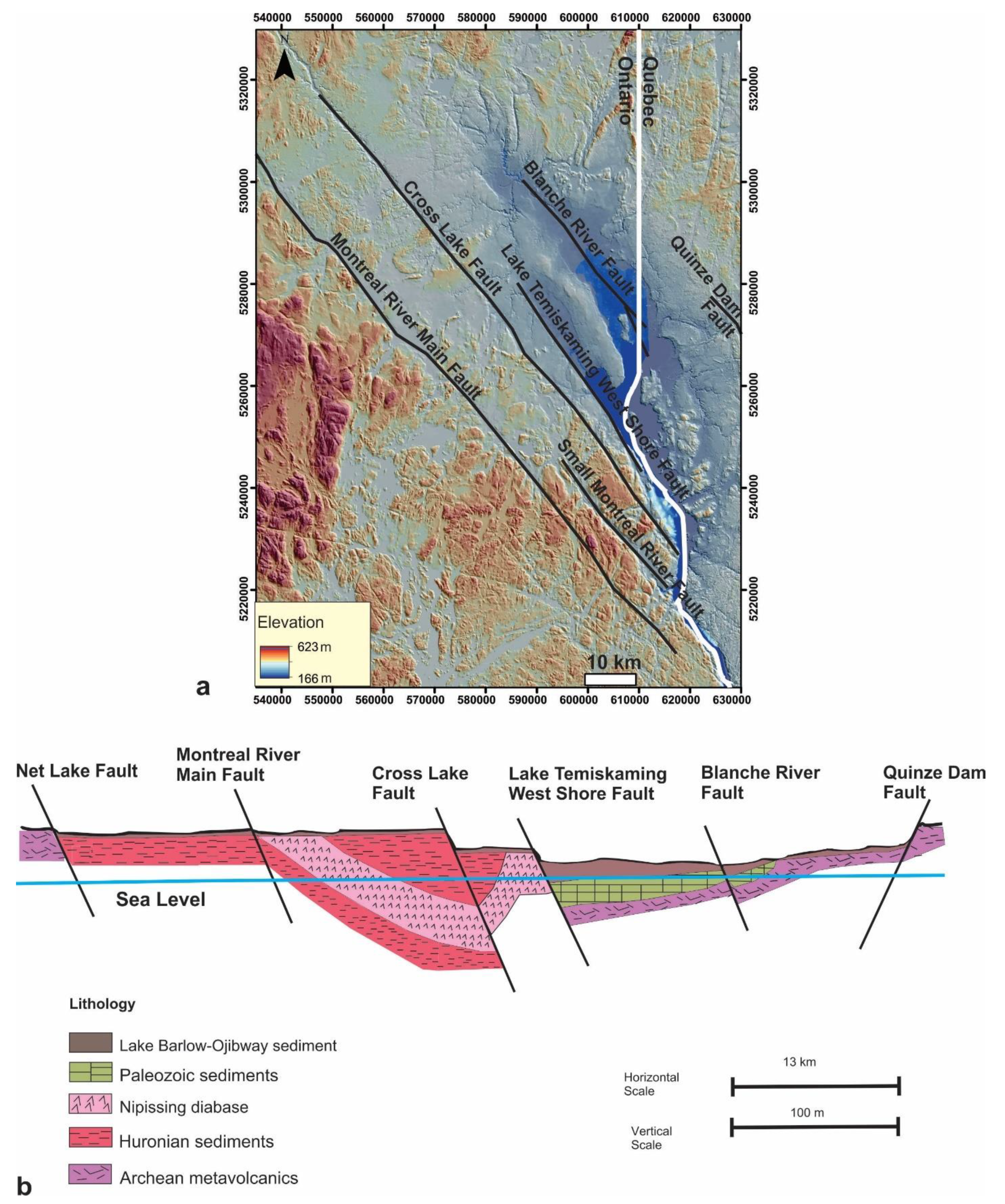
2. Study Area, General Physiography and Previous Studies

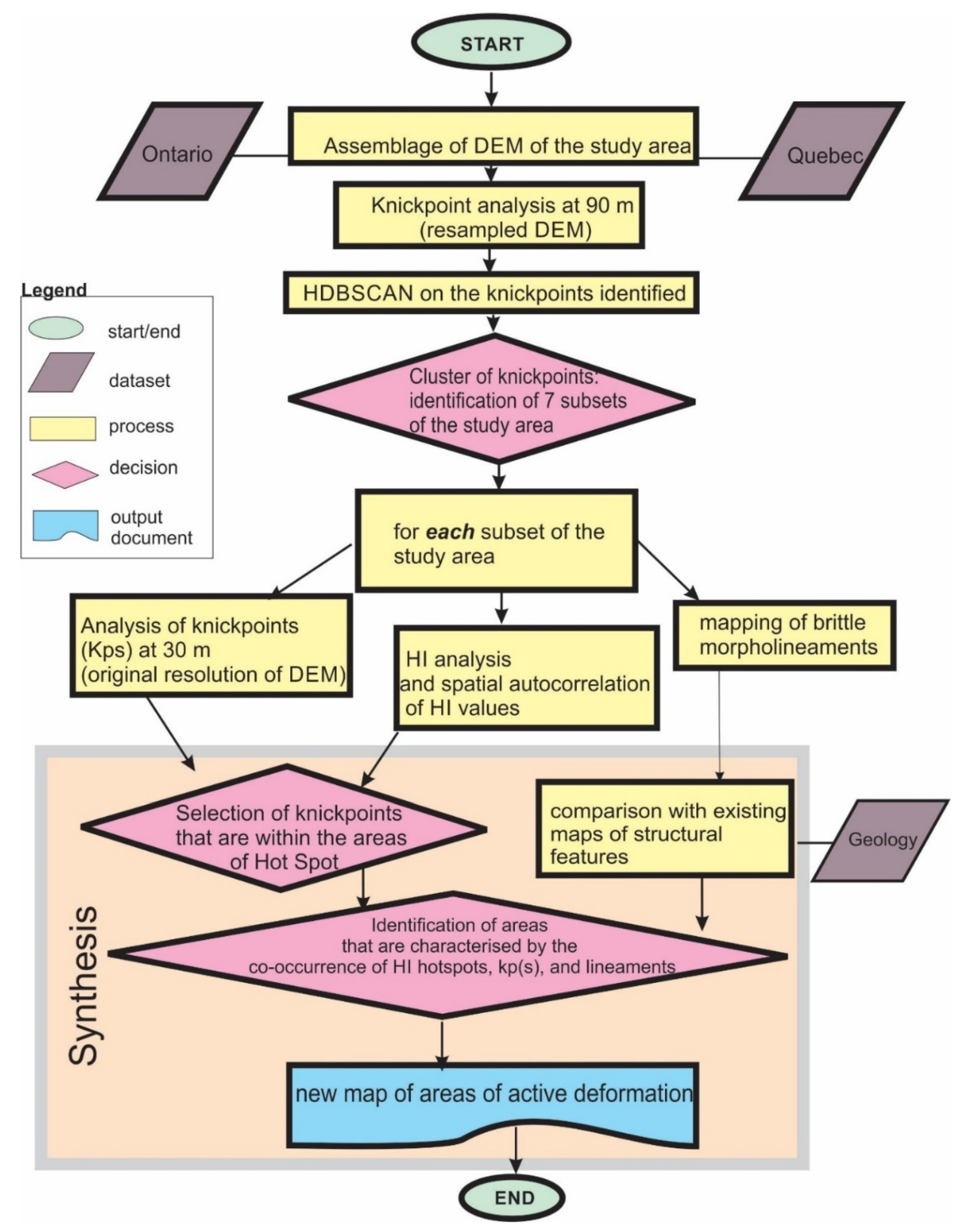
Our study area encompasses nearly 147 square km straddling the border of Ontario and Quebec, Eastern Canada. The major structural element of this area is the ‘Temiskaming Graben’ or ‘Lake Temiskaming Rift Valley’ (Lovell and Caine, 1970) within the NW portion of the Western Quebec Seismic Zone (WQSZ). The WQSZ extends from the Ottawa Valley, including the cities of Montreal and Ottawa, up to Temiskaming (or Temiscaming, or Timiskaming). It includes the eastern portion of Quebec and western portion of Ontario, around the area of the Temiskaming Graben (Figure 1 and Figure 2). We will refer to our study area as the Temiskaming Graben (TG).

The Temiskaming Graben (TG) lies within the Superior province, underlain by rocks of the Canadian Shield. The graben is a complex Paleoproterozoic structural feature [15], thought to be an analogue of the modern Western African Rift [61,62]. Early studies show that the Temiskaming Graben is affected by neotectonic structures and is therefore a weak zone within the North American continent [15]. The Temiskaming Graben is structurally defined by NW striking faults within the Paleozoic basement, with the center occupied by the modern Lake Temiskaming [63] (Figure 2). The Cross Lake Fault is centered on the Nipissing Diabase intrusion (Figure 2 [63]). To the south, the Temiskaming Graben is truncated by the tectonic zone of the Grenville Front ([64], see also Figure 2 in [65] and references therein). The Blanche River valley forms the northeastern boundary of the Temiskaming Graben, with the Blanche River fault striking parallel to the Lake Timiskaming West Shore Fault. The down-faulted portions of the Temiskaming graben are now filled with fine grained sediment known as the ‘Little Clay Belt,’ deposited when glacial Lake Barlow-Ojibway, the predecessor to the modern Temiskaming Lake, occupied the Temiskaming Graben between 10570 and 8125 BP [66,67] during the retreat of the Laurentide Ice Sheet (LIS). The Little Clay Belt is delimited towards the northeast by the Quinze Dam Fault and to the SW by the Cross Lake Fault.

Figure 2. Structural elements characterizing the Temiskaming Graben. (a) 30 m ALOS DEM overland with Hillshade map (illumination from 45°) that highlights the lineaments; (b) simplified geological cross section of the Temiskaming Graben from [63] (note that the Net Lake Fault is not represented in (a)).

Figure 2. Structural elements characterizing the Temiskaming Graben. (a) 30 m ALOS DEM overland with Hillshade map (illumination from 45°) that highlights the lineaments; (b) simplified geological cross section of the Temiskaming Graben from [63] (note that the Net Lake Fault is not represented in (a)).

Although the Temiskaming Graben is characterized by reduced seismic frequency compared with the rest of the WQSZ [68,69,70], the M 6.2, 1935 Temiskaming earthquake was one of the strongest that occurred within the region [65,71,72]. The region was then affected by the Mn 5.2 Kipawa earthquake event in January of 2000 [73], which was felt as a strong event within a radius of 50 km but with only minor damage recorded [74].

The last decade has seen a wealth of geophysical and neotectonics investigations centered on Lake Temiskaming, which is nearly 100 km long and reaches a depth of 200 m. Seismic acoustic and chirp surveys of the lake bottom [42,75,76] reveal that the basement of the lake is characterized by horst and graben structures that cut through Ordovician units, Pleistocene deposits of glacial Lake Barlow, and Holocene deposits of Lake Temiskaming [75]. Another investigation documents the co-occurrence of landslides and slumps within the 600 km² area around the earthquake’s epicenter, providing independent evidence that the Mw 6.3 1935 earthquake caused widespread effects across the landscape [65].

3. Methods

Tectonic geomorphology identifies changes in the landscape caused by the interplay between tectonic and climatic drivers by measuring specific topographic markers and geomorphic patterns. The working methodologies that characterize tectonic geomorphic studies have almost exclusively been developed in tectonically active areas with significant topography, where tectonically-induced anomalies and deviations from the expected trend of development of the landscape are more dramatically expressed [77,78,79,80,81]. However, these techniques have not been well refined for use in areas with a gentle topography and low or moderately low seismic activity. For example, river steepness (k_sn) has been extensively used to identify neotectonic activity in tectonically active regions around the world [82,83,84,85]. However, at our study site this index returned consistently low values (k_sn < 10), which made its use as a proxy for neotectonic deformation unpractical. Consequently, we investigated other tools that could be used for detecting anomalies in the landscape ascribed to structural deformation, developing a methodology that leverages the different sensitivities of three complimentary morphometric techniques. No metric clearly identifies tectonic deformation in areas with a low topographic gradient and low or moderate seismicity, but the combination of metrics yields meaningful results. We describe below the techniques we identified as most valuable and present an overview of our general workflow. The detailed explanation of the individual steps of the workflow are described in the sections that follow (3.1–3.4). We used the following three techniques:

(1) Knickpoint analysis: Knickpoints highlight anomalies along the river profile that can mark lithologic discontinuities, structural features, or changes in base level associated with climatic or tectonic perturbations [82,86,87,88]

(2) Hypsometric integral: This index evaluates the distribution of area at different elevations within a landscape; a high hypsometric integral value, for example, implies much of the landscape is perched above incised valleys and may have experienced ongoing or recent tectonic uplift from which it has not yet equilibrated [89]. This value can be calculated for a single basin, or can be calculated across the landscape using a moving window [90,91,92].

(3) Lineaments: Linear features in the landscape could reflect fault scarps, but also differential erosion along geologic contacts, or geomorphic features such as eskers or terrace risers. In this paper, we focused on linear features that could result from tectonic activity [93,94,95].

Since our study area is large, we began our workflow (Figure 3) with the assumption that although there may be many origins for knickpoints, fault displacement at the surface would generate knickpoints, and so any region of the study area without knickpoints could be excluded from our study. We therefore made a first pass across the landscape to identify knickpoints on a 90 m DEM. This resolution was more realistic for computation than the original 30 m DEM given the large size of our study area. We identified seven geographic knickpoint clusters for further investigation by applying HDBSCAN cluster analysis. For each subset, a new knickpoints analysis was run at the original resolution of the DEM (30 m) to refine the location of the knickpoints formerly identified at 90 m, and to define their density within each cluster, making the same assumption that tectonic activity would be marked by knickpoints. For each subset we also calculated the hypsometric integral using a moving window of 160,000 m² with the assumption that tectonically active areas would be marked with a high hypsometric integral. By finding the convergence of these two data sets (knickpoints and then hypsometric integral analysis), we identified areas that could be tectonically active. More importantly, at this stage, we could exclude areas with low hypsometric integrals and in which knickpoints are absent, and where we could confidently say that tectonic activity is also absent or not currently observed. These results were then integrated with a map of lineaments in the landscape, assuming that any tectonically active faults would have some topographic expression. The lineaments were compared with the known structural features mapped in the landscape. Again, lineaments may have many origins in the landscape, but by finding the convergence of lineaments with areas identified as possibly tectonically active using our other methods (knickpoints and hypsometric integral), we targeted the features most likely to be tectonically active, and conversely excluded linear features which likely do not have a tectonic origin.

3.1. Data Available and DEM Preparation

The study area straddles the Ontario–Quebec border. Digital Elevation Model datasets from provincial agencies were combined for the purpose of this investigation. We used the Ontario Provincial DEM (PDEM)-South, which is open source from the Ontario GeoHub [96], with a resolution of 30 m; it is based on data obtained through different sources, including LiDAR, radar, and contour maps [96]. We also retrieved a LiDAR-derived DTM from Foret Ouverte [97] for the Quebec side of our study area with a resolution of 5 m. We resampled this dataset at 30 m and merged it with the Ontario PDEM-South to obtain complete coverage of the study area. We used this combined dataset for surface analysis in ArcGIS, extracting major topographic attributes (e.g., Hillshade, Aspect, Slope, and Curvatures) and completing raster calculations. Finally, we also worked with the ALOS DEM dataset, which is open source with a resolution of 30 m [98], to carry out hydrological and knickpoint analysis with Topotoolbox, a Matlab-based software package [99,100]. The ALOS DEM is characterized by a reduced degree of roughness for the area considered in this analysis and therefore is best suited for hydrological purposes [101]. We further smoothed the ALOS DEM with a median filter, applied through the software PCI Geomatica, to reduce artifacts in longitudinal river profiles created by sharp edges occurring in the DEM. Note that smoothing can be accomplished with the function GRIDobj/filter in TopoToolbox, but as this feature was undocumented at the time we carried out our analysis (Schwanghart, pers comm), we used PCI Geomatica, and the results were identical. The dataset set for our analysis was plotted using the NAD 1983 Datum, UTM 17 N Zone, Transverse Mercator Projections.

The whole dataset was resampled at 90 m resolution the first stage of knickpoints investigation. This resolution was found suitable to reduce computational time while still successfully identifying areas of interest for further analysis at a finer resolution.

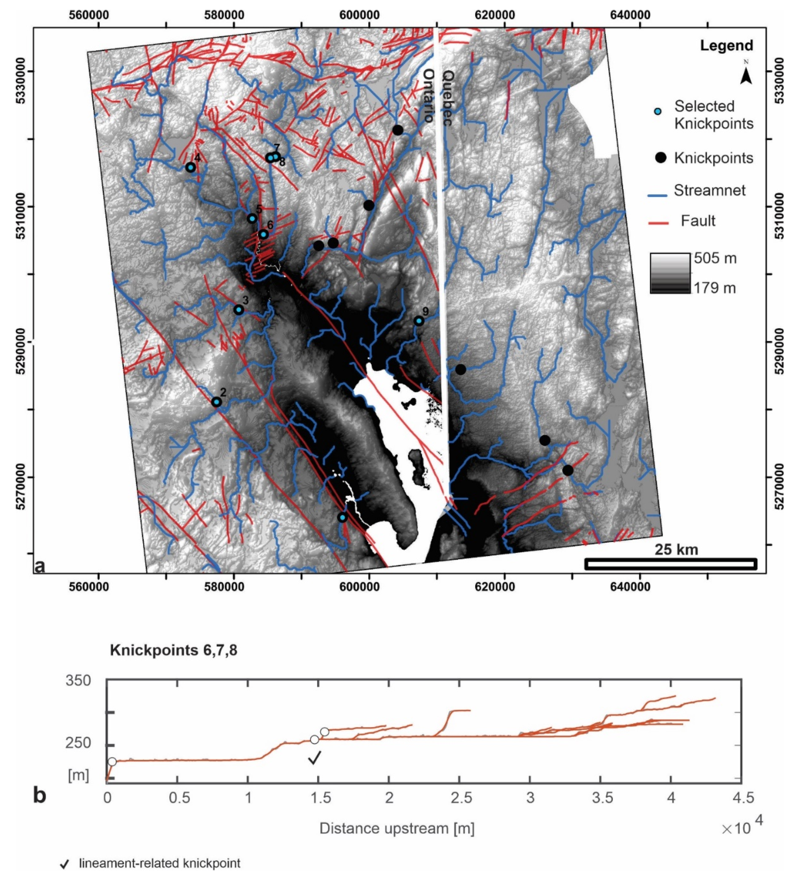
3.2. Knickpoint Analysis

River networks, and in particular, river longitudinal profiles, are sensitive to changes in tectonic or climatic activity, and to their interaction [82]. Longitudinal river profiles show variations in channel gradient by plotting stream elevation versus distance. Bedrock rivers can be described by the detachment limited model, in which erosion is limited by the ability to remove and entrain material from the bed [102,103]. In these systems, the steady state (when erosion equals uplift) morphology of the river profile is controlled by the resistance of the channel substrate to erosion and relative base level fall [104], resulting in a characteristic concave-up profile (equilibrium profile, as defined in [105,106]). The equilibrium profile is the result of the relationship between discharge and slope gradient necessary to generate the minimum shear stress that allows sediment to be detached and moved along by the channel flow [87,107]. However, smooth profiles can be interrupted by abrupt changes in slope called knickpoints, or broader changes called knickzones, both of which can be accompanied by upstream vs. downstream changes in slope relative to a given drainage area. Two types of knickpoints have been identified in the literature: slope break knickpoints that are typically associated with transient changes in the landscape, such as base level fall, and vertical step knickpoints that often reflect lithologic or tectonic contacts [104].

Knickpoint analysis was performed using the fully automated knickpoint finder tool in the MATLAB-based software TopoToolbox [101,108]. The knickpoint finder tool uses a non-parametric quantile regression (CRS: constrained regularized smoothing) that identifies the data uncertainties embedded in the DEM and contributes to smoothing the river profile. The tool then models the selected river profile. Steps for this computation entail the calculation of the Flow Direction through the function FLOWobj, embedded in TopoToolbox, followed by the calculation of the stream network with a minimum supporting drainage area of 1000 pixels. Subsequently, the code narrows the calculation to the largest component of the main drainage basin identified and the knickpoints are then extracted from the major trunk. The final result of this code was a structure array that retains information about the number and location (elevation and coordinates) of knickpoints found in that specific drainage basin. The visual outcome of this code was a plot of all the knickpoints along the river profile (Figure 4), but also of the knickpoints on the original DEM uploaded in the program.

Once we completed this preliminary scan, we performed a cluster analysis to identify promising targets for more detailed study using the function HDBSCAN in ArcGIS PRO (v 2.4). HDBSCAN (Hierarchical density-based cluster selection) is a cluster analysis that identifies similarities between points based on their spatial attributes and is effective for removing noise. This cluster analysis is particularly useful for geospatial datasets, as it does not identify clusters based on their shapes, but rather as a function of the number of objects within a region (density) in comparison to its surroundings [109]. Our analysis identified seven knickpoint clusters. We therefore focused the rest of our analysis on these seven areas, assuming that areas without knickpoints are without significant or recent tectonic activity.

We then repeated our knickpoint analysis within each of these seven areas, but using the original 30 m resolution of the DEM, but with a supporting drainage area of 10,000 pixels, in order to improve the efficiency of computation. The code was also modified in order to analyze longitudinal river profiles not only on the trunk rivers, but also on the tributaries (Section S4.2 in the Supplementary Materials).

3.3. Hypsometric Index Analysis

Hypsometry is the distribution of an area with respect to elevation within a drainage basin or across a landscape [89]. The distribution of elevation within a landscape is the result of constructive and destructive forces that derive from the interplay of tectonics, lithology, and climatic agents. It can be used, for example, to identify landscapes that have experienced recent uplift, typically characterized by a greater area of the landscape at a higher elevation, sometimes forming high-elevation, low-relief surfaces [89]. A related metric, the Hypsometric Index (HI), is the area under the hypsometric curve. Refs. [97,110] showed that the HI can also be formulated as an Elevation–Relief ratio according to the following equation,

$$HI=\frac{h_{mean}-h_{min}}{h_{max}-h_{min}}$$

(1)

where $h_{mean}$ is the mean value of the elevation,$h_{min}$ is the minimum value of elevation, and $h_{max}$ is the maximum value of elevation over a specific sampled area. High values of HI are indicative of broad elevated surfaces, while low values are indicative of isolated areas of relief [97]. Several authors have investigated the sensitivity of the HI index to tectonic and lithological variations, pointing out that uplifted areas could be detected using HI [111,112,113,114]. An effective regional approach for revealing abrupt changes in the landscape was developed by computing the HI within a fractal framework that does not consider the basin or sub-basin geometry, but rather a portion of the study area delimited by a square ([115] later defined as moving window in [59]). This approach is effective for describing the landscape and revealing abrupt changes in elevation across the study area [115]. Ref. [91] further refined the use of this technique using spatial autocorrelation statistics [116] in the Granada basin, in Spain. The authors tested the assumption that despite the high heterogeneity observed in the HI values across the study area, if tectonic forces were subtly influencing the landscape, high values or low values of HI would tend to cluster together. Spatial autocorrelation statistics highlight Hot Spot clusters where neotectonic deformation is mostly likely to occur [91]. This workflow was validated in tectonically active and high-relief areas like the Otago region, South Island of New Zealand [91], the Hindu Kush in Pakistan [92], and the northern Apennines in Italy [117], and also in areas of moderate–high relief and in intracratonic regions such as Eastern Germany and Poland [59].

We undertook HI analysis using a moving window approach for each of the seven subsets identified in our initial knickpoint analysis. The moving window must be large enough to be representative of the study area and should contain the major geomorphic elements that characterize the landscape of the study area, not being influenced by local topographic variations [59,118]. Most geomorphic parameters display a stable pattern for analysis with a moving window between 100 and 250 pixels in area [59]. Therefore, we chose a moving window for this study of 177 pixels, which covers an area of 160,000 m², considering the original 30 m resolution of our DEM. We used zonal statistics in the Spatial Analysis toolbox of ArcGIS 10.7.1 to calculate mean, minimum, and maximum values of HI. 3.3.1 Lithological information extracted and HI analysis.

Since lithologic effects can mask tectonic activity and thus alter the tectonic inference that is possible to detect through the HI [111,114], we compared HI values derived from the lithologic group in our seven subsets to lithologic data obtained from bedrock and Quaternary geology maps from Ontario [119,120] and Quebec [121]. We classified rocks as bedrock consisting dominantly of gneiss, granite, and other igneous and metamorphic rocks mostly of Precambrian age; unconsolidated sedimentary strata of mostly Pleistocene age; and glacial features of mostly Holocene age. Area 7 (on the Quebec side) was not covered by any detailed geological information, and hence no HI extraction was performed for this subset. For all the other subsets, summary statistics were computed in ArcGIS and excel.3.3.2 Spatial Statistics.

Following the methodology proposed by [91], initial values of HI were used to run Global Moran’s I statistics [122]. This statistic estimates the probability that the HI values have a random distribution (the null hypothesis of the test), with outputs of expected index value, the z score, and the p-value. The p-value assesses whether the null hypothesis can be rejected. Considering a confidence interval of 99%, the smaller the p-value, the stronger is the probability that the HI values are not randomly distributed, thus highlighting geospatial trends. Results from the Global Moran’s I statistics reveal then the geospatial significance of the distribution of our variables, but do not provide information about how high values and low values of this variable cluster in space and cannot reveal the trend of HI values. Therefore the methodological approach proposed by [91] also makes use of the Getis Ord G statistics [123]. The latter quantifies the statistical significance of each value of HI within each moving window, in comparison with the HI values of the neighboring moving windows, revealing hot and cold spot clusters of HI values that gather high values of HI and low values of HI, respectively. For the mathematical details of the Moran’s I and Getis Ord G statistics applied in this study, the reader is referred to [91] and references therein. Both the Global Moran’s I index and Getis Ord G were run in ArcGIS with a fully automated process, using the method of the Inverse Distance. We calculated the distance as Euclidean, with a threshold of 2000 m.

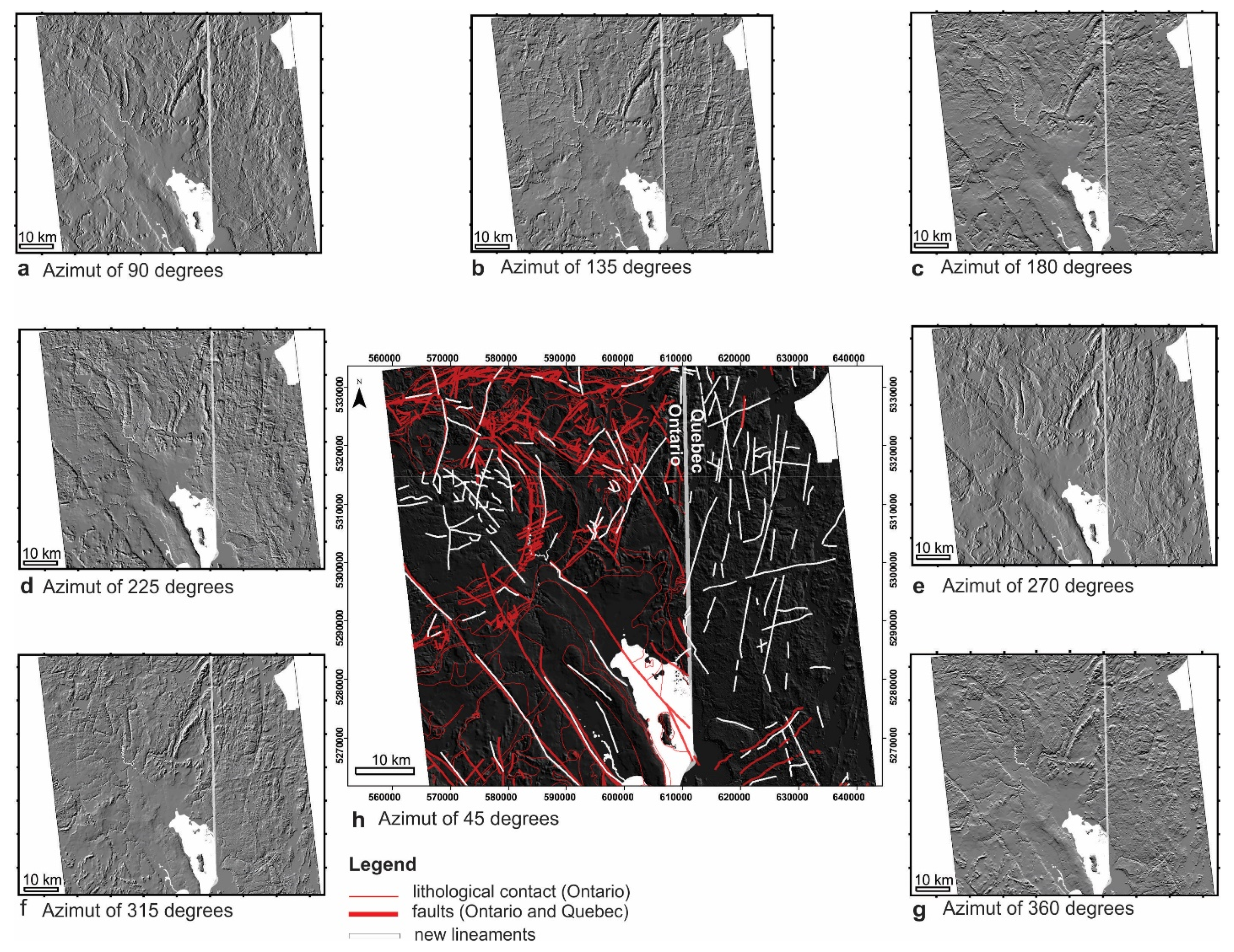
3.4. Lineament Mapping

In addition to our analysis of knickpoint distribution and regional variations in HI, we investigated the presence of lineaments in the landscape. These could reflect a variety of features, including glacial moraines or eskers, river terrace risers, eroded lithological contacts, or active or inactive faults. Lineament mapping has been widely used for mineral deposit research and in glacial landscapes [13,46,95,124,125,126,127,128]. In the last few years with the advent of machine learning techniques and increased availability of image analysis software, lineament mapping has become more efficient. Several attempts have been made to develop semi-automatic or automatic tools for lineament mapping that would reduce the bias of hand mapping [94,109,129,130,131]. However, hand mapping is the only existing protocol that guarantees very high resolution mapping, reducing the high number of artifacts that are typically produced with automatic techniques, and supports structural analysis onshore [93,94,104,127] and offshore [132].

We defined lineaments (or morpholineaments) as any linear topographic discontinuity. We identified and hand mapped morpholineaments only in the seven study areas identified through our knickpoint analysis from the scale of 1:26,000 through to 1:300,000. We produced eight hillshade maps calculated with a sun altitude of 10 degrees and azimuths of 45°, 90°, 135°, 180°, 225°, 270°, 315°, and 360° for each area [129]. The sun altitude of 10 degrees was found to be particularly useful for our landscape, which is dominated by bedrock, as suggested by [129]. Lineaments with different orientations are highlighted by these different illumination directions. The lineaments were observed and mapped on each of the eight hillshades, then combined into one shapefile. Lineaments were identified as features with a strong visual marker (i.e., shadow on the DEM), with low sinuosity and curvature, and a length of at least 5 m. Features were merged into a final dataset, with features identified on more than one hillshade consolidated to a single feature. We calculated the cardinal compass direction of each lineament using the spatial statistics toolbox in ArcGIS 10.7., which allowed us to extract the frequency and orientation of each linear feature. We also tested an automatic and a semi-automatic extraction of lineament mapping using PCI Geomatica software. However, the occurrence of a high number of artifacts made the use of this method inefficient for the purpose of this research.

4. Results

4.1. Analysis of Knickpoints at 90 m, and HDBSCAN

We detected 187 knickpoints on the 90 m resolution dataset (Figure 4). This analysis allowed us to identify areas of knickpoint concentration. Knickpoints are concentrated in the northern sector of the study area, where a moderately high change in elevation occurs along one of the major rivers of the area. Other areas where the knickpoints are more densely concentrated are coincident with changes in gradient (for example on the western side of the study area), or are concentrated along the eastern and western shores of Temiskaming Lake (Figure 4).

HDBSCAN analysis identified seven clusters obtained from 90 m resolution data. The major physiographic aspects of the seven subsets are summarized in the Table S1 in the Supplementary Materials.

4.2. Analysis of Knickpoints at 30 m

We identified 146 knickpoints in the seven subsets using our 30 m dataset. The location of the knickpoints was checked against the location of hydraulic and related anthropogenic structures [133]; based on this analysis we only removed one knickpoint, n 2 within area 1, because it is coincident with a hydraulic station (Figure S1). No other knickpoints were found coincident with anthropogenic structures. Drainage basins were identified within each of the seven subsets to isolate the river network on which the knickpoints occur, and in order to plot them on their respective longitudinal river profiles. We include results from Subset 5 here as representative of the type of results obtained from each subset (Figure 5), with results for the other subsets available in the Supplementary Materials (Figures S1–S8). A detailed compendium of the major morphometric features characterizing only the selected knickpoints (the knickpoints at 30 m resolution falling within the HI Hot Spot areas) is presented in

Table 1. Selected knickpoints characteristics.

Subset Number	Total (Selected) Knickpoints *	Drainage Basin Number	Basin Area (km2)	Knickpoint Number	Knickpoint Coordinates UTM 17N (x, y)	Knickpoint Elevation (m)
1	14 (7)	1	877	1	400,806.7, 5,542,635.6	161
		2	1670	2	454,866.7, 5,558,415.6	120
				3	457,776.7, 5,539,965.6	178
		3	1704	4	478,596.7, 5,554,065.6	189
		4	1933	5	497,226.7, 5,561,445.6	204
		5	2054	6	513,636.7, 5,574,645.6	208
				7	523,146.8, 5,570,235.6	235
2	9 (8)	1	2072	1	367,942.6, 5,317,836.4	398
				3	371,581.6, 5,319,170.7	396
				7	376,433.6, 5,321,596.6	418
				5	382,498.5, 5,326,448.6	414
		2	360	2a	344,653.2, 5,315,895.6	383
				2b	351,931.2, 5,325,963	375
		3	2796	6	404,089.7, 5,301,097.1	377
				8	402,270.2, 5,304,978.7	380
3	34 (13)	1	2525	1	439,956.88, 5,211,825.6	430
				2	437,406.8, 5,174,925.6	369
				3	434,736.8, 5,165,175.6	398
				4	446,676.8, 5,172,135.6	337
		2	3095	5	470,826.8, 5,161,335.6	318
				6	491,616.8, 5,178,675.6	390
				7	495,036.8, 5,199,135.6	387
		3	2077	8	504,246.8, 5,227,365.6	358
				9	506,346.8, 5,215,305.6	359
				10	508,986.8, 5,210,445.6	344
				11	508,446.8, 5,202,075.6	358
				12	509,526.8, 5,200,245.6	350
		4	1131	13	550,146.8, 5,237,655.6	339
4	6 (2)	1	737	1	607,566.8, 5,157,975.6	339
				2	590,886.8, 5,158,545.6	287
5	16 (9)	1	60	1	596,106.8, 5,264,025.6	273
		2	507	2	577,476.8, 5,281,095.6	238
				3	580,776.8, 5,294,715.6	270
		3	620	4	573,666.8, 5,315,775.6	229
				5	582,756.8, 5,308,185.6	228
		4	300	6	584,406.8, 5,305,845.6	230
				7	585,426.8, 5,317,185.6	289
				8	586,206.8, 5,317,335.6	258
		5	210	9	607,386.8, 5,293,065.6	224
6	23 (10)	1	247	1	613,206.8, 5,219,805.6	275
		2	28	2	615,966.8, 5,216,565.6	250
		3	22	3	625,866.8, 5,202,105.6	250
		4	371	4	641,616.8, 5,156,355.6	309
		5	81	5	644,856.8, 5,169,855.6	288
		6	33	6	642,966.8, 5,173,095.6	308
		7	57	7	639,606.8, 5,182,545.6	308
				8	640,956.8, 5,182,515.6	243
		8	99	9	645,996.8, 5,176,725.6	242
		9	36	10	654,906.8, 5,161,335.6	238
7	46 (25)	1	219	1	219,770.5, 5,157,043.7	333
				2	220,215.3, 5,153,397.4	296
		2	330	3	225,693.9, 5,135,973.0	213
				4	226,903.2, 5,137,627.1	249
				5	225,283.1, 5,136,907.3	256
		3	96	6	234,806.6, 5,134,287.9	243
		4	562	7	245,344.6, 5,135,534.6	250
				8	243,243.8, 5,144,722.7	259
		5	58	9	250,373.5, 5,130,819.5	205
				10	252,410.9, 5,132,289.8	277
		6	91	11	257,903.6, 5,130,518.9	211
				12	260,474.6, 5,129,902.6	238
		7	21	13	267,077.2, 5,126,904.6	220
		8	38	14	275,095.2, 5,125,123.3	226
		9	2238	15	286,829.4, 5,139,815.3	215
				16	283,708.0, 5,141,887.4	255
				17	284,753.3, 5,148,907.2	296
				18	281,756.5, 5,150,639.3	286
				19	288,210.5, 5,155,201.7	300
				20	283,970.1, 5,159,164.6	297
				21	292,577.3, 5,163,953.1	323
				22	288,747.9, 5,170,140.9	336
		10	380	23	302,283.2, 5,121,107.4	271
				24	296,645.01, 5,121,715.1	209
				25	302,575.4, 5,127,340.7	273

* Total number of knickpoints reflects number identified on 30 m DEM for each subset. Selected number reflects knickpoints that fall within HI Hot Spot areas and/or correspond with mapped lineaments.

. Drainage basins are not shown in the maps of Figure 5 and in Figures S1–S8 in order to simplify the layout of the final map, but the area covered by each is provided in Table 1.

4.3. HI Results

Raster calculation of the HI resulted in a poorly informative map (Figure 6a). In a few cases (Subsets 3 and 5), high values of HI lie along mapped fault structures, but generally, the HI values are not consistently grouped around structural or lithological features and are therefore not useful for identifying neotectonic structures. Hot Spot statistics obtained through Getis Ord analysis on HI values, however, are valuable (Figure 6b). The Hot Spots represents clusters of high values of HI that often cover areas large enough to incorporate more than one mapped structural feature (see for example Subsets 3 and 5 where this is particularly evident). Cold Spots identify areas where moderate or low values of HI values are grouped together. Cold Spot areas are not only coincident with lower elevations within the landscape (e.g., valleys incised by rivers) but they could also be coincident with faults or other lithological contacts already mapped by the OGS or the QGS. This means that both Hot Spot and Cold Spot areas could reflect neotectonic activity. HI values do not appear to be influenced by lithological discontinuities (Figure 6c) (Tables S3 and S4 and Figures S15 and S16, see other HI analysis for the other subset areas in the Supplementary Materials in Figures S9–S14).

4.4. Lineaments Hand Mapping

We identified a total of 2197 lineaments across the seven subsets, ranging in length from few tens of meters to several kilometers in length, with a mean value of 4 km (Table S5). Where available, we integrated our mapping of lineaments with the map of structural features (and thus also lineaments) in published geologic maps provided by the OGS and QGS [119,120,121] (Figure 7). In most cases the lineaments identified are exploited by the river network. We identified two major trends (Figure 7 and Figure 8 and Figures S17–S19): N-S striking lineaments dominate subsets for Area 1 (41.4%), Area 2 (37.4%), and Area 5 (43.2%), while a NW-SE component dominates in Area 4 (52.1%) and Area 6 (43.2%). Both orientations are pronounced in Area 3 (NW–SE 29.6%; N–S 28.8%) and Area 7 (NW–SE 29.8%, N–S 17.1%) (Figure 8). Our results are consistent with previous analysis of lineament trends and mapping of the broad region of Temiskaming that attempt to link lineament trend with the fault plane orientation and the regional stress field [20,74,128].

4.5. Synthesis

For each subset, we synthesized the results of our knickpoint, hypsometric, and lineament analysis in order to identify the most likely areas of neotectonic activity. We focused on knickpoints that fall within areas of HI Hot Spots (Table 1), producing a longitudinal profile for each river with an associated knickpoint (Figures S1–S8). Most knickpoints were located along the trunk rivers, but we also analyzed tributary profiles and associated knickpoints (see Section S4.2 in Supplementary Materials). Longitudinal profiles are graded (smooth) for subsets 1, 5, 6, and 7. In Subsets 2, 3, 4 and partially also 5, the longitudinal river profiles are affected by a step stair morphology that could partially reflect artifacts in the DEM in flat areas (Schwanghart et al., 2013; Schwanghart and Scherler, 2017), but could also be explained by the higher concentration of brittle fractures cutting through these rivers networks.

Using the co-occurrence of knickpoints, lineaments, and HI Hot Spots, we identified ‘Areas of Interest’ (AoI) for further neotectonics investigation. An overview of the synthesis procedure for Subset 5 is presented in Figure 9 and summarized in Figure 10 for all the other areas. Every ‘AoI’ could potentially represent a newly identified area of active deformation. A new cluster analysis at this stage is not appropriate (e.g., HDBSCAN, see Section 3) since some of the knickpoints are located far apart (see Figure 9 as an example) and this type of cluster analysis, based on the density of the point features, will not include into specific clusters potential knickpoints that are adjacent instead to rather than on newly or pre-existing lineaments, and within Hot Spot areas of HI, thus invalidating our initial assumptions and the results obtained so far.

5. Discussion

5.1. Summary of the Key Findings and Validation of our Technique

Our workflow can be validated against regions in which neotectonic structures are well known. Unfortunately, only one such area with sufficient data on active structures exists in the understudied Western Quebec Seismic Zone: Area 5, which encompasses the Temiskaming Graben (Figure 9). In this region, selected knickpoints are on or adjacent to known structural features of the Temiskaming Graben. Our lineament analysis identified the major faults in the area with the exception of the Blanche River Fault. The HI Hot Spot overlaps and aligns with the Cross Lake, Lake Temiskaming West Shore, and Blanche River faults. Knickpoint 2 lies along the Cross Lake Fault, knickpoints 2 and 3 lie on or closely adjacent to the Lake Temiskaming West Shore fault, and knickpoints 4 through 8 lie in a region of complex lineaments and mapped faults along strike, and to the north of the mapped Blanche River Fault. Only knickpoint 9 cannot be definitively linked to a known fault or mapped lineament. Further field investigations are warranted for all of the identified Areas of Interest, but in particular the areas around knickpoint 9 merits further study.

Our analysis of the other six subsets suggests likely targets of interest. We highlight four cases in particular. In subset 1 (Figure 10a), which is the northern part of our study area, a number of knickpoints (1, 2–5, 6) were aligned NE–SW with known structures, although only two knickpoints are actually coincident with mapped faults. This could reflect the existence of multiple, parallel fault strands or misplacement of the precise location of mapped faults. Notably the lineaments we identified in this study do not align with these knickpoints or the known faults. A similar situation occurs in subset 2 in the western part of our study area (Figure 10b), with knickpoints 1, 3, 5, and 7 aligned NE–SW with known structures, but poorly aligned with lineaments mapped in this study. This location therefore warrants further study. In subset 3 (Figure 10c), a promising set of knickpoints (8–12) were aligned N–S along newly mapped lineaments. Targets in the other three areas are less promising given that they are not as concentrated and do not show good alignment with each other or mapped lineaments or faults. Additionally, HI analysis and the related Getis Ord G* analysis did not result in extensive HI Hot Spot areas in subset 4 (Figure S12), due potentially to the large coverage of water bodies within the DEM of the study area, which created a high number of Cold Spot or not significant areas. Subsets 6 (Figure 10e) is characterized by a high number of isolated knickpoints but knickpoints 7 and 8 align with a regional known fault. Subset 7 (Figure 10f) is characterized by a high number of knickpoints that are coincident with lineaments. In particular, knickpoints 1–2, 19–20, and 21–22 are coincident with lineaments oriented NE–SW. This subset is the only area that was not characterized by a regional fault map; therefore, further field studies and geophysical investigations are needed for investigating the structural features outlined here.

5.2. Considerations about the Techniques

Identifying subregions where subtle tectonic deformation occurs in areas with no obvious evidence of surface rupture, postglacial faults, or steep topographic gradients that could highlight the occurrence of structures is challenging. Therefore, this study promotes the synergistic use of three different techniques: knickpoint analysis, calculation of the Hypsometric Integral using a moving window, and lineament mapping. This study suggests that only the co-occurrence of results obtained by the three techniques provide a robust analysis of the subregion capable of identifying ‘Areas of Interest’ where potential tectonic activity has been identified. Due to the nature of the work, each of the areas considered ‘of interest’ (see Figure 10) should be ground-truthed with geophysical and geological analysis to identify evidence of displacement or offset in the subsurface. Further, a high-quality DEM is critical for this study. DEMs are characterized by a high number of artifacts, in particular in areas of lows relief, and that could interfere with hydrological analysis of the dataset [101,134]. For this reason, it is important to corroborate hydrological investigation (knickpoints detection) with other tools such as HI analysis and lineament mapping. The next step is to further validate our morphometric investigation with structural geology and shallow geophysics for assessing the existence of the features that could be responsible for the subtle neotectonic deformation suggested by our analysis.

This contribution is the first of its kind at the time of writing to perform a tectonic geomorphic analysis in an area with a gentle gradient and low elevation. This workflow could also be applied in other areas with seismicity but that are low relief or with an overall gentle topographic gradient (for example the Ottawa–Bonnechere Graben). It will likely also be useful in urbanized areas to address threats to infrastructure (e.g., nuclear facilities or hydropowers). Despite that the recommended workflow is long and requires access to MATLAB and software for hydrological and geospatial analysis (ArcGIS, and ArcGIS pro), this type of analysis is still considered efficient and especially useful for identifying areas of neotectonic interest in low-seismic and gentle-gradient landscapes.

6. Conclusions

We identified areas throughout our study site in the Temiskaming region, characterized by knickpoints, hypsometric indices, and lineaments clusters. The validation of these anomalies against known faults of the Temiskaming region demonstrates that they likely represent areas of neotectonic activity. Our multi-step methodology represents a valuable contribution in the field of tectonic-geomorphology because it extends the application of classic tectono-geomorphologic techniques to low relief, low elevation, and moderately low tectonic activity study areas. The newly identified areas of likely active deformation can be targeted for further analysis using geophysics, structural geology, and paleoseismology, for example in other sectors of the WQSZ (in particular St Lawrence Graben) where the current seismicity is more concentrated.

References

1. Bruneau, M.; Lamontagne, M. Damage from 20th century earthquakes in eastern Canada and seismic vulnerability of unreinforced masonry buildings. Can. J. Civ. Eng. 1994, 21, 643–662. [Google Scholar] [CrossRef]
2. Lamontagne, M. An overview of some significant Eastern Canadian earthquakes and their impacts on the geological environment, buildings and the public. Nat. Hazards 2002, 26, 55–67. [Google Scholar] [CrossRef]
3. Adams, J.; Wetmiller, R.J.; Hasegawa, H.S.; Drysdale, J. The first surface faulting from a historical intraplate earthquake in North America. Nature 1991, 352, 617–619. [Google Scholar] [CrossRef]
4. Ebel, J.E.; Tuttle, M.P. Earthquakes in the Eastern Great Lakes Basin from a regional perspective. Tectonophysics 2002, 353, 17–20. [Google Scholar] [CrossRef]
5. Lamontagne, M.; Halchuk, S.; Cassidy, J.F.; Rogers, G.C. Significant Canadian earthquakes 1600–2006. Seismol. Res. Lett. 2007, 79, 211–223. [Google Scholar] [CrossRef]
6. Bent, A.L.; Lamontagne, M.; Peci, V.; Halchuk, S.; Brooks, G.; Motazedian, D.; Hunter, J.A.; Adams, J.; Woodgold, C.; Drysdale, J.; et al. The 17 May 2013 M 4.6 Ladysmith, Quebec, Earthquake. Seismol. Res. Lett. 2015, 86, 460–476. [Google Scholar] [CrossRef]
7. Bent, A.L.; Peci, V.; Halchuk, S.; Hayek, S. Two moderate earthquakes near Montreal: 10 October and 6 November 2012. Seismol. Res. Lett. 2014, 85, 940–947. [Google Scholar] [CrossRef]
8. Ma, S.; Audet, P. The 5.2 magnitude earthquake near Ladysmith, Quebec, 17 May 2013: Implications for the seismotectonics of the Ottawa–Bonnechere Graben. Can. J. Earth Sci. 2014, 51, 439–451. [Google Scholar] [CrossRef]
9. Basham, D.M.; Weichert, D.H.; Berry, M.J. Regional assessment of seismic risk in eastern Canada. Bull. Seismol. Soc. Am. 1979, 11, 1567–1602. [Google Scholar]
10. Forsyth, D.A. Characteristics of the Western Quebec Seismic Zone. Can. J. Earth Sci. 2011, 18, 103–119. [Google Scholar] [CrossRef]
11. Ma, S.; Eaton, D.W. Western Quebec seismic zone (Canada): Clustered, midcrustal seismicity along a Mesozoic hot spot track. J. Geophys. Res. 2007, 112, B06305. [Google Scholar] [CrossRef] [Green Version]
12. Shilts, W.W. Sonar evidence for postglacial tectonic instability of the Canadian Shield and Appalachians. Geol. Surv. Can. 1984, 84, 567–579. [Google Scholar]
13. Goodacre, A.K.; Bonham-Carter, G.F.; Agterberg, F.P.; Wright, D.F. A statistical analysis of the spatial association of seismicity with drainage patterns and magnetic anomalies in western Quebec. Tectonophysics 1994, 217, 285–305. [Google Scholar] [CrossRef]
14. Rimando, R.E.; Benn, K. Evolution of faulting and paleo-stress field within the Ottawa graben, Canada. J. Geodyn. 2005, 39, 337–360. [Google Scholar] [CrossRef]
15. Mazzotti, S. Geodymanic models for earthquake studies in intraplate North America. In Continental intraplate Earthquakes: Science, Hazard, and Policy Issues; Stein, S., Mazzotti, S., Eds.; Special Paper; Geological Society of America: Boulder, CO, USA, 2007; Volume 425, pp. 17–33. [Google Scholar]
16. Zoback, M.L. Stress field constraints on intraplate seismicity in eastern North America. J. Geophys. Res. Solid Earth 1992, 97, 11761–11782. [Google Scholar] [CrossRef] [Green Version]
17. Stein, S. Approaches to continental intraplate earthquake issues. In Continental Intraplate Earthquakes; Stein, S., Mazzotti, S., Eds.; Science, hazard, and Policy Issue; Geological Society of America Special Papers; Geological Society of America: Boulder, CO, USA, 2007; Volume 425, pp. 1–16. [Google Scholar]
18. Mazzotti, S.; Townend, J. State of stress in central and eastern North American seismic zones. Lithosphere 2010, 2, 76–83. [Google Scholar] [CrossRef] [Green Version]
19. Peace, A.L.; Dempsey, E.D.; Schiffer, C.; Welford, J.K.; McCaffrey, K.J.; Imber, J.; Phethean, J.J. Evidence for basement reactivation during the opening of the Labrador Sea from the Makkovik Province, Labrador, Canada: Insights from field data and numerical models. Geosciences 2018, 8, 308. [Google Scholar] [CrossRef] [Green Version]
20. Rimando, J.; Peace, A.L. Reactivation potential of intraplate faults in the Western Quebec Seismic Zone, Eastern Canada. Earth Space Sci. 2021, 8, e2021EA001825. [Google Scholar] [CrossRef]
21. Galadini, F.; Galli, P.; Giraudi, C. Geological investigations of Italian earthquakes: New paleoseismological data from the fucino plain (Central Italy). J. Geodyn. 1997, 24, 87–103. [Google Scholar] [CrossRef]
22. Galli, P.; Galadini, F.; Calzoni, F. Surface Faulting in Norcia (Central Italy): A Paleoseismological Perspective. Tectonophysics 2005, 403, 117–130. [Google Scholar] [CrossRef]
23. Caputo, R.; Poli, M.E.; Minarelli, L.; Rapti, D.; Sboras, S.; Stefani, M.; Zanferrari, A. Paleoseismological evidence for the 1570 Ferrara earthquake, Italy: Evidence of the 1570 Ferrara earthquake. Tectonics 2016, 35, 1423–1445. [Google Scholar] [CrossRef]
24. Cinti, F.R.; Civico, R.; Blumetti, A.M.; Chiarini, E.; La Posta, E.; Pantosti, D.; Papasodaro, F.; Smedile, A.; De Martini, P.M.; Villani, F.; et al. Evidence for surface faulting earthquakes on the Montereale fault system (Abruzzi Apennines, central Italy). Tectonics 2018, 37, 2758–2776. [Google Scholar] [CrossRef]
25. Okumura, K. Paleoseismology of the Itoigawa-Shizuoka tectonic line in central Japan. J. Seismol. 2001, 5, 411–431. [Google Scholar] [CrossRef]
26. Lin, A.; Sano, M.; Wang, M.; Yan, B.; Bian, D.; Fueta, R.; Hosoya, T. Paleoseismic study of the Kamishiro Fault on the northern segment of the Itoigawa–Shizuoka Tectonic Line, Japan. J. Seismol. 2017, 21, 683–703. [Google Scholar] [CrossRef] [PubMed] [Green Version]
27. Miyashita, Y. Holocene paleoseismic history of the Yunodake fault ruptured by the 2011 Fukushima-ken Hamadori earthquake, Fukushima Prefecture, Japan. Geomorphology 2018, 323, 70–79. [Google Scholar] [CrossRef]
28. Bastin, S.; van Ballegooy, S.; Mellsop, N.; Wotherspoon, L. Liquefaction case histories from the 1987 Edgecumbe earthquake, New Zealand—Insights from an extensive CPT dataset and paleo-liquefaction trenching. Eng. Geol. 2019, 271, 105404. [Google Scholar] [CrossRef]
29. Bastin, S.H.; Quigley, M.C.; Bassett, K.; Green, R.A. Characterisation of Modern and Paleo-Liquefaction Features in Eastern Christchurch, NZ, Following the 2010–2011 Canterbury Earthquake Sequence, NZ Geomechanics News; New Zealand Geotechnical Society: Wellington, New Zealand, 2013; Volume 26, pp. 38–46. [Google Scholar]
30. Villamor, P.; Almond, P.; Tuttle, M.P.; Giona Bucci, M.; Langridge, R.M.; Clark, K.; Ries, W.; Bastin, S.H.; Eger, A.; Vandergoes, M.; et al. Liquefaction features produced by the 2010–2011 Canterbury earthquake sequence in southwest Christchurch, New Zealand and preliminary assessment of paleoliquefaction features. Bull. Seismol. Soc. Am. 2016, 106, 1747–1771. [Google Scholar] [CrossRef] [Green Version]
31. Tuttle, M.P.; Villamor, P.; Almond, P.; Bastin, S.; Giona Bucci, M.; Langdridge, R.; Clark, K.; Hardwick, C. Liquefaction induced by the 2010–2011 Canterbury, New Zealand, earthquake sequence and lessons learned for the study of paleoliquefaction features. Seismol. Res. Lett. 2017, 88, 1403–1414. [Google Scholar] [CrossRef]
32. Tuttle, M.P.; Cowie, P.; Wolf, L. Liquefaction induced by modern earthquakes as a key to paleoseismicity: A case study of the 1988 Saguenay earthquake. In Proceedings of the Nineteenth International Water Reactor Safety Information Meeting, Bethesda, MD, USA, 28–30 October 1991; Weiss, A., Ed.; Volume 3, pp. 437–462. [Google Scholar]
33. Tuttle, M.P.; Lafferty, R.H.; Schweig, E.S. Dating of liquefaction features in the New Madrid Seismic Zone and implication for earthquake Hazard; Report NUREG/GR-0017; US Nuclear Regulatory Commission: Rockville, MD, USA, 1998. [Google Scholar]
34. Tuttle, M.P. Towards a Paleoearthquake Chronology for the New Madrid Seismic Zone: Collaborative Research; M. Tuttle & Associates and Central Region Geologic Hazards Team, USGS: Georgetown, ME, USA, 2001. [Google Scholar]
35. Tuttle, M.P.; Atkinson, G.M. Localization of large earthquakes in the Charlevoix seismic zone, Quebec, Canada during the past 10,000 years. Seismol. Res. Lett. 2010, 81, 18–25. [Google Scholar] [CrossRef]
36. Tuttle, M.P.; Hartleb, R.; Wolf, L.; Mayne, P.W. Paleoliquefaction studies and the evaluation of Seismic Hazard-review. Geosciences 2019, 9, 311. [Google Scholar] [CrossRef] [Green Version]
37. Brooks, G.R. A massive sensitive clay landslide, Quyon Valley, southwestern Québec, Canada, and evidence for a paleoearthquake triggering mechanism. Quat. Res. 2013, 80, 425–434. [Google Scholar] [CrossRef]
38. Brooks, G.R. Evidence of late glacial paleoseismicity from submarine landslide deposits within Lac Dasserat, northwestern Quebec, Canada. Quat. Res. 2016, 86, 184–199. [Google Scholar] [CrossRef]
39. Brooks, G.R. Deglacial record of palaeoearthquakes interpreted from mass transport deposits at three lakes near Rouyn-Noranda, north-western Quebec, Canada. Sedimentology 2018, 65, 2439–2467. [Google Scholar] [CrossRef]
40. Brooks, G.R.; Pugin, A.J.-M. Assessment of a seismo-neotectonic origin for the New Liskeard–Thornloe scarp, Timiskaming graben, northeastern Ontario. Can. J. Earth Sci. 2019, 57, 267–274. [Google Scholar] [CrossRef]
41. Brooks, G.R.; Adams, J. A review of evidence of glacially-induced faulting and seismic shaking in eastern Canada Quaternary. Sci. Rev. 2020, 228, 106070. [Google Scholar] [CrossRef]
42. Doughty, M.; Eyles, C.H.; Eyles, N.; Wallace, K.; Boyce, J.I. Lake sediments as natural seismographs: Earthquake-related deformations (seismites) in central Canadian lakes. Sediment. Geol. 2014, 313, 45–67. [Google Scholar] [CrossRef]
43. Adams, J. Postglacial faulting in eastern Canada: Nature, origin and seismic hazard implications. Tectonophysics 1989, 163, 323–331. [Google Scholar] [CrossRef]
44. Lagerback, R. Dating of Late Quaternary faulting in northern Sweden. J. Geol. Soc. 1992, 149, 285–291. [Google Scholar] [CrossRef]
45. Morner, N.A.; Troften, P.E.; Sjoberg, R.; Grant, D.; Dawson, S.; Bronge, C.; Kvamsdal, O.; Siden, A. Deglacial paleoseismicity in Sweden: The 9663 BP Iggesund event. Quat. Sci. Rev. 2000, 19, 1461–1468. [Google Scholar] [CrossRef]
46. Morner, N.A. An interpretation and catalogue of paleoseismicity in Sweden. Tectonophysics 2005, 408, 265–307. [Google Scholar] [CrossRef]
47. Lagerback, R.; Sundh, M. Early Holocene Faulting and Paleoseismicity in Northern Sweden; Geological Survey of Sweden: Uppsala, Sweden, 2018. [Google Scholar]
48. Ojala, A.E.K.; Mattila, J.; Markovaara-Koivisto, M.; Ruskeeniemi, T.; Palmu, J.-P.; Sutinen, R. Distribution and morphology of landslides in northern Finland: An analysis of postglacial seismic activity. Geomorphology 2019, 326, 190–201. [Google Scholar] [CrossRef]
49. Kujansuu, R. Nuorista siirroksista Lapissa. English summary: Recent faults in Lapland. Geologi 1964, 16, 30–36. [Google Scholar]
50. Lundqvist, J.; Lagerbäck, R. The Pärve Fault: A late-glacial fault in the Precambrian of Swedish Lapland. Geol. Föreningen I Stockh. Förhandlingar 1976, 98, 45–51. [Google Scholar] [CrossRef]
51. Lagerback, R.; Henkel, H. Studier av Neotektonisk Aktivitet i Mellersta och Norra Sverige, Flygbildsgenomga˚ng och Geofysisk Tolkning av Recenta Fo¨rkastningar; Swedish Nuclear Fuel and Waste Management Company, KBS: Stockholm, Sweden, 1977. [Google Scholar]
52. Lagerback, R. Neotectonic structures in northern Sweden. Geol. Föreningen Stockh. Förhandlingar 1978, 100, 263–269. [Google Scholar] [CrossRef]
53. Olesen, O. The Stuoragurra Fault, evidence of neotectonics in the Precambrian of Finnmark, northern Norway. Nor. Geol. Tidskr. 1988, 68, 107–118. [Google Scholar]
54. Steffen, H.; Olesen, O.; Sutinen, R. Glacially-Triggered Faulting; Cambridge University Press: Cambridge, UK, 2021. [Google Scholar]
55. Muir Wood, R. Extraordinary deglaciation reverse faulting in northern Fennoscandia. In Earthquakes at NorthAtlantic Passive Margins: Neotectonics and Postglacial Rebound; Gregersen, S., Basham, P.W., Eds.; Kluwer: Dordrech, The Netherlands, 1989; pp. 141–173. [Google Scholar]
56. Arvidsson, R. Fennoscandian earthquakes: Whole crustal rupturing related to postglacial rebound. Science 1996, 274, 744–746. [Google Scholar] [CrossRef]
57. Adams, J. Crustal stresses in eastern Canada. In Neotectonics and Postglacial Rebound, Volume Earthquakes at North Atlantic Passive Margins: Dordrecht; Gregersen, S., Basham, P.W., Eds.; NATO ASI Series; Springer: Dordrecht, The Netherlands, 1989; Volume 266, pp. 289–297. [Google Scholar]
58. Adams, J.E.; Basham, P.W. The seismicity and seismotectonics of eastern Canada. In Neotectonics of North America; Slemmons, D.B., Engdhal, E.R., Zoback, M.D., Blackwell, D.D., Eds.; Geological Society of America: Boulder, CO, USA, 1991; Volume 1. [Google Scholar]
59. Andreani, L.; Stanek, K.P.; Gloaguen, R.; Krentz, O.; Domínguez-González, L. DEM-based analysis of interactions between tectonics and landscapes in the Ore Mountains and Eger Rift (East Germanyand NW Czech Republic). Remote Sens. 2014, 6, 7971–8001. [Google Scholar] [CrossRef] [Green Version]
60. Gioia, D.; Schiattarella, M.; Giano, S.I. Right-angle pattern of minor fluvial networks from the Ionian Terraced Belt, Southern Italy: Passive structural control or foreland bending? Geosciences 2018, 8, 331. [Google Scholar] [CrossRef] [Green Version]
61. Freund, R. Rift Valleys, The World Rift System; Geological Survey of Canada: Ottawa, ON, Canada, 1966. [Google Scholar]
62. Kumarapeli, P.S.; Saul, V.A. The St. Lawrence Valley system: A North American equivalent of the East African Rift System. Can. J. Earth Sci. 1966, 3, 639–658. [Google Scholar] [CrossRef]
63. Lovell, H.R.; Caine, T.W. Lake Timiskaming Rift Valley; Ontario Department of Mines and Northern Affairs: Toronto, ON, Canada, 1970. [Google Scholar]
64. Dix, G.R.; Coniglio, M.; Riva, J.F.V. The Late Ordovician Dawson point formation (Timiskaming outlier, Ontario): Key to a new regional synthesis of Richmondian-Hirnantian carbonate and siliclastic magna facies across the central Canadian craton. Can. J. Earth Sci. 2007, 28, 1349–1352. [Google Scholar] [CrossRef]
65. Doughty, M.; Eyles, N.; Daurio, L. (1935 Timiskaming M6.2) triggered slumps in Lake Kipawa, Western Quebec Seismic Zone, Canada. Sediment. Geol. 2010, 228, 113–118. [Google Scholar] [CrossRef]
66. Dyke, A.S. An outline of North American deglaciation with emphasis on central and northern Canada. In Quaternary Glaciations-Extent and Chronology, Part II; Ehlers, J., Gibbard, P.L., Eds.; Elsevier: Amsterdam, The Netherlands, 2004; pp. 373–424. [Google Scholar]
67. Godbout, P.-M.; Roy, M.; Veillette, J.-J. High-resolution varve sequences record one major late-glacial ice readvance and two drainage events in the eastern Lake Agassiz-Ojibway basin. Quat. Sci. Rev. 2019, 223, 105942. [Google Scholar] [CrossRef]
68. Dufréchou, G.; Harris, L.B. Tectonic models for the origin of regional transverse structures in the SW Grenville Province interpreted from regional gravity. J. Geodyn. 2013, 64, 15–39. [Google Scholar] [CrossRef]
69. Dufréchou, G.; Harris, L.B.; Corriveau, L. Tectonic reactivation of transverse basement structures in the Grenville orogen of SW Quebec, Canada; insights from gravity and aeromagnetic data. Precambrian Res. 2014, 241, 61–84. [Google Scholar] [CrossRef]
70. Harris, L.B.; Dufréchou, G. Localization of the intraplate Western Quebec—Adirondack Mountains seismic zone of N America by deep Precambrian structures, transverse to the Grenville Orogen. In Proceedings of the Biennial Conference, Thredbo NSW, Geological Society of Australia, Thredbo, Australia, 2–8 February 2014. [Google Scholar]
71. Hodgson, E.A. The Temiskaming earthquake of November 1, 1935. The location of the epicentre and determination of focal depth. J. R. Astron. Soc. Can. 1936, 30, 113–123. [Google Scholar]
72. Doig, R. Effect of strong seismic shaking in lake sediments and earthquake recurrence interval, Temiskaming, Quebec. Can. J. Earth Sci. 1991, 28, 1349–1352. [Google Scholar] [CrossRef]
73. Adams, J.; Bent, A.; Drysdale, J.; Halchuck, S.; Lamontagne, M.; Ma, S.; Wentmiller, R.J.; Woodgold, C.; Dastous, J.-B. The 01 January 2000 Kipawa Earthquake (MN = 5.2); Geological Survey of Canada: Ottawa, ON, Canada, 2000. [Google Scholar]
74. Bent, A.L.; Lamontagne, M.; Adams, J.; Woodgold, C.R.D.; Halchuk, S.; Drysdale, J.; Wetmiller, R.J.; Ma, S.; Dastous, J.-B. The Kipawa, Québec “Millennium” Earthquake. Seismol. Res. Lett. 2002, 73, 285–297. [Google Scholar] [CrossRef]
75. Doughty, M.; Eyles, N.; Eyles, C.H. High-resolution seismic reflection profiling of neotectonic faults in Lake Timiskaming, Timiskaming Graben, Ontario-Quebec, Canada. Sedimentology 2013, 60, 983–1006. [Google Scholar] [CrossRef]
76. Doughty, M.; Eyles, N.; Daurio, L. Ongoing neotectonic activity in the Timiskaming–Kipawa Area of Ontario and Québec. Geosci. Can. 2010, 37, 109–116. [Google Scholar]
77. Burbank, D.W.; Pinter, N. Landscape evolution: The interaction of tectonics and surface processes. Basin Res. 1999, 11, 1–6. [Google Scholar] [CrossRef]
78. Burbank, D.W.; Anderson, R.A. Tectonic Geomorphology; Blackwell Science: Malden, MA, USA, 2001. [Google Scholar]
79. Bull, W.B. Tectonic Geomorphology of Mountains; Blackwell Publishing: Malden, MA, USA, 2017. [Google Scholar]
80. Ascione, A.; Cinque, A.; Miccadei, E.; Villani, F.; Berti, C. The Plio-Quaternary uplift of the Apennine chain: New data from the analysis of topography and river valleys in central Italy. Geomorphology 2008, 102, 105–118. [Google Scholar] [CrossRef] [Green Version]
81. Watkinson, I.M.; Hall, R. Fault systems of the eastern Indonesian triple junction: Evaluation of Quaternary activity and implications for seismic hazards. In Geohazards in Indonesia: Earth Science for Disaster Risk Reduction; Cummins, P.R., Meilano, I., Eds.; The Geological Society of London: London, UK, 2017; Volume 441, pp. 71–120. [Google Scholar]
82. Kirby, E.; Whipple, K.X. Expression of active tectonics in erosional landscapes. J. Struct. Geol. 2012, 44, 54–75. [Google Scholar] [CrossRef]
83. Chen, Y.-W.; Shyu, J.B.H.; Chang, C.P. Neotectonic characteristics along the eastern flank of the Central Range in the active Taiwan orogen inferred from fluvial channel morphology. Tectonics 2015, 34, 2249–2270. [Google Scholar] [CrossRef]
84. Vanacker, V.; von Blanckenburg, F.; Govers, G.; Molina, A.; Campforts, B.; Kubik, P.W. Transient river response, captured by channel steepness and its concavity. Geomorphology 2015, 228, 234–243. [Google Scholar] [CrossRef] [Green Version]
85. Siddiqui, S.; Castaldini, D.; Soldati, M. DEM-based drainage network analysis using steepness and Hack SL indices to identify areas of differential uplift in Emilia–Romagna Apennines, northern Italy. Arab. J. Geosci. 2017, 10, 1–23. [Google Scholar] [CrossRef]
86. Wobus, C.; Whipple, K.X.; Kirby, E.; Snyder, N.; Johnson, J.; Spyropolou, K.; Crosby, B.; Sheehan, D. Tectonics from Topography: Procedures, Promise and Pitfalls; Geological Society of America Special Paper; No. Penrose Conference Series; Geological Society of America: Boulder, CO, USA, 2006; Volume 398, pp. 55–74. [Google Scholar]
87. Pavano, F.; Pazzaglia, F.J.; Catalano, S. Knickpoints as geomorphic markers of active tectonics: A case study from northeastern Sicily (southern Italy). Lithosphere 2016, 8, 633–648. [Google Scholar] [CrossRef] [Green Version]
88. Marra, F.; Frepoli, A.; Gioia, D.; Schiattarella, M.; Tertulliani, A.; Bini, M.; De Luca, G.; Luppichini, M. A morpho-tectonic approach to the study of earthquakes in Rome. Nat. Hazards Earth Syst. Sci. Discuss 2022. preprint. [Google Scholar]
89. Strahler, A.N. Hypsometric (area-altitude) analysis of erosional topography. Geol. Soc. Am. Bull. 1952, 63, 1117–1142. [Google Scholar] [CrossRef]
90. Pike, J.R.; Wilson, S.E. Elevation-Relief Ratio, Hypsometric Integral, and geomorphic area-altitude analysis. Geol. Soc. Am. Bull. 1971, 82, 1079–1084. [Google Scholar] [CrossRef]
91. Perez-Pena, J.V.; Azano, J.M.; Booth-Rea, G.; Azor, A.; Delgado, J. Differentiating geology and tectonics using a spatial autocorrelation technique for the hypsometric integral. J. Geophys. Res. 2009, 114, F02018. [Google Scholar] [CrossRef]
92. Mahmoud, S.; Gloaguen, R. Analysing spatial autocorrelation for the hypsometric integral to discriminate neotectonics and lithologies using DEMs and GIS. GIScience Remote Sens. 2011, 48, 541–565. [Google Scholar] [CrossRef]
93. Morelli, M.; Piana, F. Comparison between remote sensed lineaments and geological structures in intensively cultivated hills (Monferrato and Langhe domains, NW Italy). Int. J. Remote Sens. 2006, 20, 4471–4493. [Google Scholar] [CrossRef]
94. Ramli, M.F.; Yusof, N.; Yusoff, M.K.; Juahir, H.; Shafri, H.Z.M. Lineament mapping and its application in landslide hazard assessment: A review. Bull. Eng. Geol. Environ. 2010, 69, 215–233. [Google Scholar]
95. Scheiber, T.; Fredin, O.; Viola, G.; Jarna, A.; Gasser, D.; Łapińska-Viola, R. Manual extraction of bedrock lineaments from high-resolution LiDAR data: Methodological bias and human perception. GFF 2015, 137, 362–372. [Google Scholar] [CrossRef] [Green Version]
96. Ontario Ministry of Natural Resources and Forestry-Provincial Mapping Unit. Provincial Digital Elevation Model (PDEM); Ontario Ministry of Natural Resources and Forestry, Ed.; Ontario Provincial Mapping, 2013. Available online: https://geohub.lio.gov.on.ca/datasets/mnrf::provincial-digital-elevation-model-pdem (accessed on 1 April 2020).
97. Gouvernement du Québec. 2015–2021, LiDAR. In Ministère des Forêts, and de la Faune et des Parcs (MFFP); Ministère des Forêts, de la Faune et des Parcs (MFFP). Available online: https://www.foretouverte.gouv.qc.ca/?context=_lidar&zoom=6&center=-70.78076,50.58378&invisiblelayers=*&visiblelayers=6954522a31346e60dd6a9ba3105a29bd,09e0a456d4ea557627fee6f6928a8e7a,b70fcde722df2f0b913374961c7c9ae8,1da64ddfeaf23710b8a9ad95133fb5d8 (accessed on 1 November 2019).
98. Earth Observation Research Center. ALOS World, 3D-30m (AW3D30) Version 3.1. 2020. Available online: https://www.eorc.jaxa.jp/ALOS/en/dataset/aw3d30/aw3d30_e.htm (accessed on 1 March 2020).
99. Schwanghart, W.; Kuhn, N.J. TopoToolbox: A set of Matlab functions for topographic analysis. Environ. Model. Softw. 2010, 25, 770–781. [Google Scholar]
100. Schwanghart, W.; Scherler, D. TopoToolbox 2–MATLAB-based software for topographic analysis and modeling in Earth surface sciences. Earth Surf. Dyn. 2014, 2, 1–7. [Google Scholar] [CrossRef] [Green Version]
101. Schwanghart, W.; Scherler, D. Bumps in river profiles: Uncertainty assessment and smoothing using quantile regression techniques. Earth Surf. Dyn. 2017, 5, 821–839. [Google Scholar] [CrossRef] [Green Version]
102. Tucker, G.E.; Whipple, K.X.J. Topographic outcomes predicted by stream erosion models: Sensitivity analysis and intermodel comparison. Geophys. Res. Solid Earth 2002, 107, ETG 1-1–ETG 1-16. [Google Scholar] [CrossRef] [Green Version]
103. Whipple, K.X.; Tucker, G.E. Implications of sediment-flux-dependent river incision models for landscape evolution. J. Geophys. Res. Solid Earth 2002, 107, ETG3-1–ETG3-20. [Google Scholar] [CrossRef] [Green Version]
104. Boulton, S.J. Geomorphic response to differential uplift: River long profiles and knickpoints from Guadalcanal and Makira (Solomon Islands). Front. Earth Sci. 2020, 8, 10. [Google Scholar] [CrossRef]
105. Hack, J.T. Studies of longitudinal stream profiles in Virginia and Maryland. US Geol. Surv. Prof. Pap. 1954, 294, 45–97. [Google Scholar]
106. Mackin, J.H. Concept of the graded river. Geol. Soc. Am. Bull. 1948, 59, 463–512. [Google Scholar] [CrossRef] [Green Version]
107. Bull, W.B. Geomorphic Responses to Climatic Change; Oxford University Press: New York, NY, USA, 1991. [Google Scholar]
108. Stolle, A.; Schwanghart, W.; Andermann, C.; Bernhardt, A.; Fort, M.; Jansen, J.D.; Wittmann, H.; Merchel, S.; Rugel, G.; Adhikari, B.R.; et al. Protracted river response to medieval earthquakes. Earth Surf. Processes Landf. 2018, 44, 331–341. [Google Scholar] [CrossRef] [Green Version]
109. Campello, R.J.G.B.; Moulavi, D.; Sander, J. Density-Based Clustering based on Hierarchical Density Estimates; Springer: Berlin/Heidelberg, Germany, 2011; pp. 160–172. [Google Scholar]
110. Wood, W.F.; Snell, J.B. A Quantitative System for Classifying Landforms; Technical Report EP-124; US Army, Quartermaster Research & Engineering Center: Natick, MA, USA, 1960. [Google Scholar]
111. Lifton, N.A.; Chase, C.G. Tectonic, climatic and lithologic influences on landscape fractal dimension and hypsometry: Implications for landscape evolution in the San Gabriel Mountains, California. Geomorphology 1992, 5, 77–114. [Google Scholar] [CrossRef]
112. Delcaillau, B.; Deffontaines, B.; Floissac, L.; Angelier, J.; Deramond, J.; Souquet, P.; Chu, H.T.; Lee, J.F. Morphotectonic evidence from lateral propagation of an active frontal fold; Pakuashan anticline, foothills of Taiwan. Geomorphology 1998, 24, 263–290. [Google Scholar] [CrossRef]
113. Chen, Y.C.; Sung, Q.; Cheng, K.-Y. Along-strike variations of morphotectonic features in the Western Foothills of Taiwan: Tectonic implications based on stream-gradient and hypsometric analysis. Geomorphology 2003, 56, 109–1137. [Google Scholar] [CrossRef]
114. Cohen, S.; Willgoose, G.; Hancock, G. A methodology for calculating the spatial distribution of the area-slopeequation and the hypsometric integral within a catchment. J. Geophys. Res. 2008, 113, F03027. [Google Scholar]
115. van der Beek, P.; Braun, J. Numerical modeling of landscape evolution on geological time-scales: A parameter analysis and comparison with the south-eastern highlands of Australia. Basin Res. 1998, 10, 49–68. [Google Scholar] [CrossRef]
116. Anselin, L. Local indicators of spatial association—LISA. Geograph. Anal. 1995, 27, 93–115. [Google Scholar] [CrossRef]
117. Siddiqui, S.; Soldati, M. Appraisal of active tectonics using DEM-based hypsometric integral and trend surface analysis in Emilia-Romagna Apennines, northern Italy. Turk. J. Earth Sci. 2014, 23, 277–292. [Google Scholar] [CrossRef]
118. Rabii, F.; Achour, H.; Rebai, N.; Jallouli, C. Hypsometric integral for the identification of neotectonic and lithology differences in low tectonically active area (Utica-Mateur region, north eastern Tunisia). Geocarto Int. 2017, 32, 1229–1242. [Google Scholar] [CrossRef]
119. Ontario Geological Survey. 1:250,000 Scale Bedrock Geology of Ontario; Ontario Geological Survey, Miscellaneous Release—Data 126-Revision 1; Ministry of Energy, and Northern Development and Mines, Ed.; Ministry of Energy, Northern Development and Mines, Ontario Geological Survey, 2011. Available online: http://www.geologyontario.mndm.gov.on.ca/mndmaccess/mndm_dir.asp?type=pub&id=MRD126-REV1 (accessed on 1 April 2020).
120. Ontario Geological Survey. Quaternary Geology, Seamless Coverage of the Province of Ontario: Ontario Geological Survey, Data Set 14; Ministry of Northern Development and Mines, Ed.; Ministry of Northern Development and Mines: Greater Sudbury, ON, Canada, 1997. Available online: http://www.geologyontario.mndm.gov.on.ca/mndmaccess/mndm_dir.asp?type=pub&id=eds014-rev (accessed on 1 April 2020).
121. Mines Service Centre. SIGEOM, Geomining Information System of Quebec; Governement of Quebec, Ministère de l’Énergie, et des Ressources Naturelles, Eds.; Mines Service Centre, 2020; Available online: http://sigeom.mines.gouv.qc.ca/signet/classes/I1102_aLaCarte?l=A (accessed on 1 April 2020).
122. Moran, P.A.P. Notes on Continuous Stochastic Phenomena. Biometrika 1950, 37, 17–23. [Google Scholar] [CrossRef]
123. Ord, J.K.; Getis, A. Local spatial autocorrelation statistics: Distributional issues and an application. Geogr. Anal. 1995, 27, 286–306. [Google Scholar] [CrossRef]
124. Jansson, K.A.; Glasser, N.F. Using Landsat 7 ETM + imagery and Digital Terrain Models for mapping glacial lineaments on former ice sheet beds. Int. J. Remote Sens. 2005, 26, 3931–3941. [Google Scholar] [CrossRef] [Green Version]
125. Smith, M.J.; Clark, C.D. Methods for the visualization of digital elevation models for landform mapping. Earth Surf. Processes Landf. 2005, 30, 885–900. [Google Scholar] [CrossRef]
126. Smith, M.J.; Rose, J.; Booth, S. Geomorphological mapping of glacial landforms from remotely sensed data: An evaluation of the principal data sources and an assessment of their quality. Geomorphology 2006, 76, 148–165. [Google Scholar] [CrossRef]
127. Santimano, T.; Riller, U. Revisiting thrusting, reverse faulting and transpression in the southern Sudbury Basin, Ontario. Precambrian Res. 2012, 200, 74–81. [Google Scholar] [CrossRef]
128. Lamontagne, M.; Brouillette, P.; Grégoire, S.; Bédard, M.P.; Bleeker, W. Faults and Lineaments of the Western Quebec Seismic Zone, Quebec and Ontario; Geological Survey of Canada: Ottawa, ON, Canada, 2020. [Google Scholar]
129. Šilhavý, J.; Minár, J.; Mentlík, P.; Sládekd, J. A new artefacts resistant method for automatic lineament extraction using Multi-Hillshade Hierarchic Clustering (MHHC). Comput. Geosci. 2016, 92, 9–20. [Google Scholar] [CrossRef]
130. Karimi, B.; Karimi, H.A. An automated method for the detection of topographic patterns at tectonic boundaries, patterns 2017. In Proceedings of the Ninth International Conference on Pervasive Patterns and Application, Athens, Greece, 19–23 February 2017. [Google Scholar]
131. Salui, C.L. Methodological validation for automated lineament extraction by LINE Method in PCI Geomatica and Matlab based Hough Transformation. J. Geol. Soc. India 2018, 92, 321–328. [Google Scholar] [CrossRef]
132. Baxter, A.T.; Hannington, M.D.; Stewart, M.S.; Emberley, J.M.; Breker, K.; Krätschell, A.; Petersen, S.; Brandl, P.A.; Klischies, M.; Mensing, R.; et al. Shallow seismicity and the classification of structures in the Lau Back-Arc Basin. Geochem. Geophys. Geosyst. 2020, 21, e2020GC008924. [Google Scholar] [CrossRef] [Green Version]
133. Statistics Canada. Electric Power Generating Stations: Natural Resources Canada. 2007. Available online: https://open.canada.ca/data/en/dataset/ce1a6040-8893-11e0-9597-6cf049291510 (accessed on 1 August 2021).
134. Schwanghart, W.; Groom, G.; Kuhn, N.J.; Heckrath, G. Flow network derivation from a high resolution DEM in a low relief, agrarian landscape. Earth Surf. Processes Landf. 2013, 38, 1576–1586. [Google Scholar] [CrossRef]
Figure 1. (a) Location of the study area within the eastern Canada, showing a broad outline of the WQSZ and the location of where our study area is located; (b) DEM of the study area between the provinces of Ontario and Quebec; (c) slope map of the study area, calculated in percent rise and location of the Mw 6.1 1935 Temiskaming earthquake (source: seismescanada.rncan.gc.ca, accessed on 1 September 2021).
Remotesensing 14 03587 g001
Figure 3. Workflow diagram for the methodology proposed in this study. We integrate multiple techniques commonly used in tectono-geomorphic studies that involve complex digital topography and hydrological analysis.
Remotesensing 14 03587 g003
Figure 4. Combined DEM of our study area centered around the Temiskaming Graben with Knickpoints detected at 90 m resolution. The DEM was resampled at 90 m resolution in order to obtain the locations of the knickpoints across the whole study area. This resolution was found efficient for the hydrological calculations run in the MATLAB based software code TopoToolbox [99,100]. HDBSCAN cluster analysis [109] was then run for further detailing our analysis and divide the broad study area into subsets. Seven clusters of knickpoints were thus obtained by the previous passage, and each of these was used to identify a subset of the broad study area (right hand side of the figure). Within each of these subsets a new knickpoint analysis was run at 30 m resolution to confirm and/or improve the resolution of the siting of the knickpoints found at 90 m. Each identified cluster at 90 m first and then at 30 m of resolution was denoted by colored symbols, and it defines a subset of the study area. The same colors for each cluster/subset area were used for the upcoming maps. The subset areas identified by the knickpoint clusters are outlined by a black rectangular shape.
Remotesensing 14 03587 g004
Figure 5. DEM and cross section of Subset 5 illustrating our analysis. (a) We identified 16 knickpoints (Table 1) at 30 m resolution within this subset (in black) but only 9 (in blue) were “selected” knickpoints because of their coincidence with HI Hot Spot areas (see explanation of the synthesis of our results in Section 4.5) and/or known structural features of the Temiskaming graben area; (b) profile for river on which knickpoints 6, 7, and 8 are found; knickpoint 7 is coincident with a known structural linear feature.
Remotesensing 14 03587 g005
Figure 6. HI analysis for Subset area 5 with geological map; (a) HI map of subset 5; (b) Getis-Ord G analysis, also known as Hot Spot Analysis, of HI, showing the occurrence of clusters of high and low values of HI, against a map of major structural features of the area and local stream network; (c) summary of the major quaternary deposits and bedrock outcrops in Ontario (Ontario Geological Survey, 1997, 2011). (Note that a comparable map for Quebec was not available at the time of writing. Similar panels for the other subsets are found in the Supplementary Materials of this paper, Figures S9–S14.
Remotesensing 14 03587 g006
Figure 7. Morpholineaments mapped in Subset 5; the hillshades from panels (ag) were calculated with a sun altitude of 10 degrees across the different azimuths; (h) compendium of all mapped lineaments in comparison with previously mapped faults and lithological contacts.
Remotesensing 14 03587 g007
Figure 8. Radial histograms depicting the orientation of the lineaments hand mapped across the seven subset areas, with related statistics. A N–S and NW–SE trend of the newly mapped linear features predominates. Details about the mapping for the other subsets can be found in the Supplementary Data (panel Figures S17–S19).
Remotesensing 14 03587 g008
Figure 9. Synthesis for Subset Area 5. (a) Location of all knickpoints obtained at the resolution of 30 m and areas of HI Hot Spot (see Figure 6b for complete autospatial correlation of HI values). The knickpoints that are completely within the red area outlined by the HI Hot Spot are “selected” knickpoints; (b) lineaments hand mapped in this study compared with known structural features [119,120,121]; (c) synthesis of the two datasets with Areas of Interest (AoI) indicated with black ovals. The AoI for this subset are coincident with known structural features, providing validation of the techniques and of the workflow that is illustrated in this contribution.
Remotesensing 14 03587 g009
Figure 10. Final maps of areas of active deformation obtained in this study according to the workflow illustrated in Figure 9 for (a) subset 1, (b) subset 2, (c) subset 3, (d) subset 4, (e) subset 6, (f) subset 7. Black ovals identify Areas of Interest, clusters of knickpoints that have a higher potential to reflect underlining neotectonic structural features.
Remotesensing 14 03587 g010