
Near-Surface NO2 Concentration Estimation by Random Forest Modeling and Sentinel-5P and Ancillary Data


Abstract
:
1. Introduction
2. Dataset Construction
2.1. Data Preparation
2.1.1. TropOMI Data
2.1.2. Meteorological Data
2.1.3. Ground Monitoring Station Data
2.2. Ground and Satellite Data Quality Control
2.2.1. Ground Data Quality Control
2.2.2. TropOMI Data Quality Control
2.3. Data Set Generation
3. Methods
3.1. Random Forest (RF) Algorithm Implementation
3.2. Evaluation Procedure
4. Establishment of Near-Surface NO2 Concentration Estimation Model
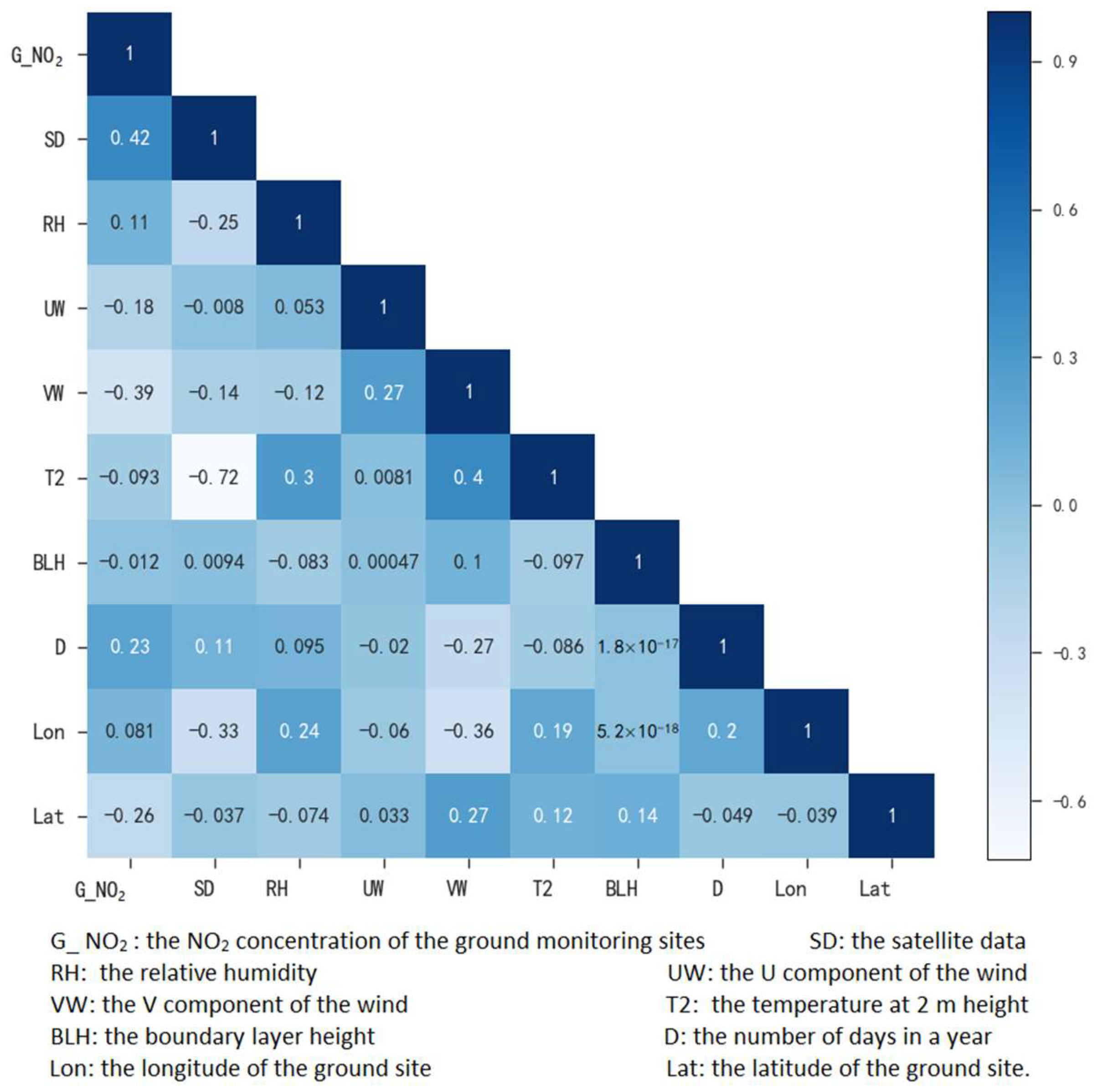
4.1. Feature Selection
4.2. Construction of the RF Platform
5. Results and Discussion
6. Conclusions
- In the daily model established to estimate the near-surface NO2 concentration in China based on the RF method, the tropospheric NO2 columns observed by TropOMI have a substantial influence on the importance of the model and the highest correlation with the near-surface NO2 concentration. It can be seen that adding satellite data into the model is helpful in estimating near-surface NO2 concentrations. Furthermore, temperature, date and NDVI also contribute to the NO2 concentration estimation near the surface.
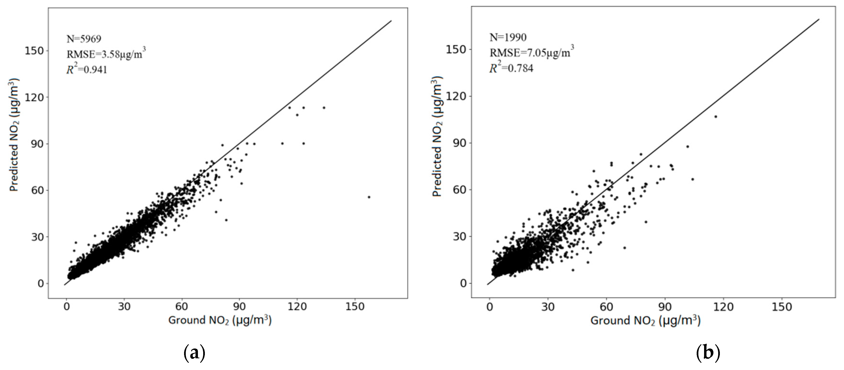
- The established model was verified based on the ten-fold cross-validation method. The R2 and RMSE of the model for estimating the daily NO2 concentration in China by the RF model are 0.78 and 7.04 μg/m3, respectively. Compared with previous studies on modeling the daily NO2 concentration, there are still some gaps in the R2 but the RMSE is an improvement.
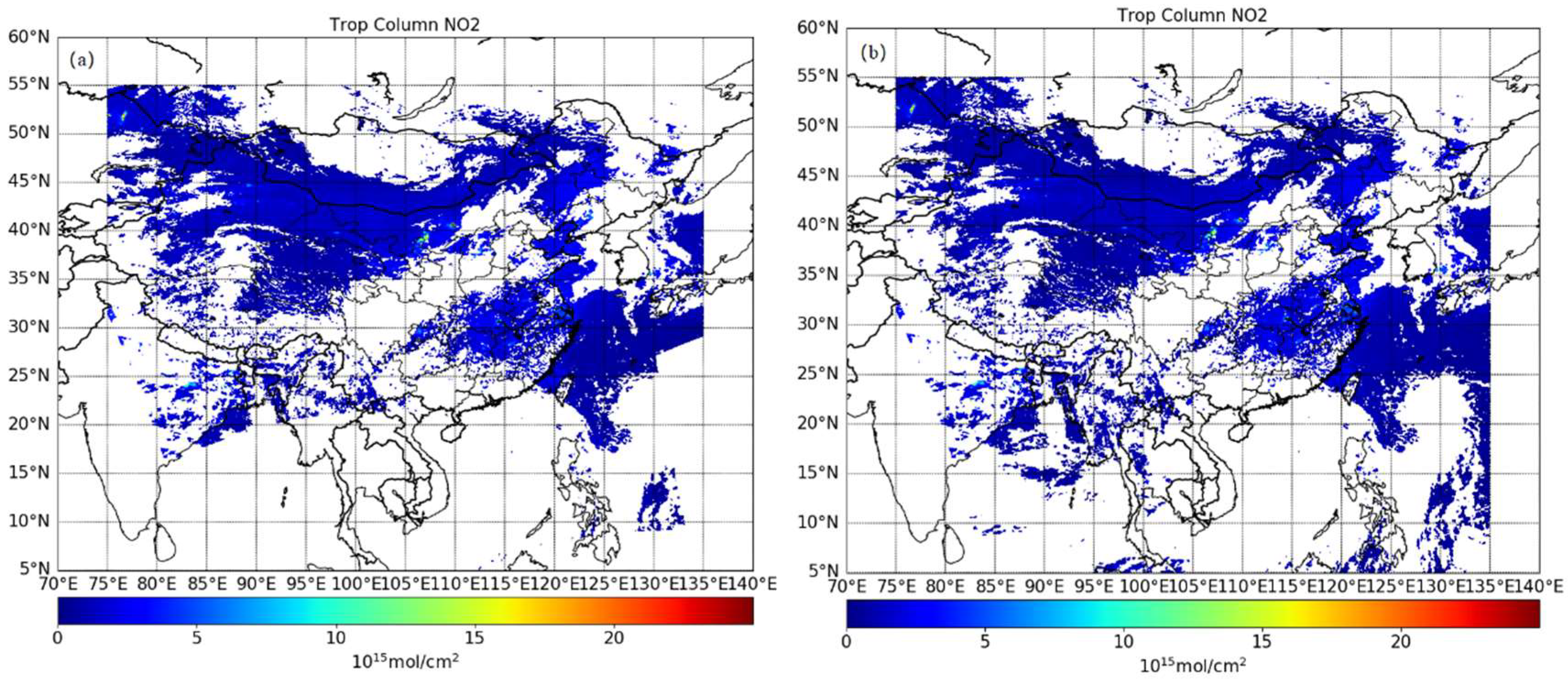
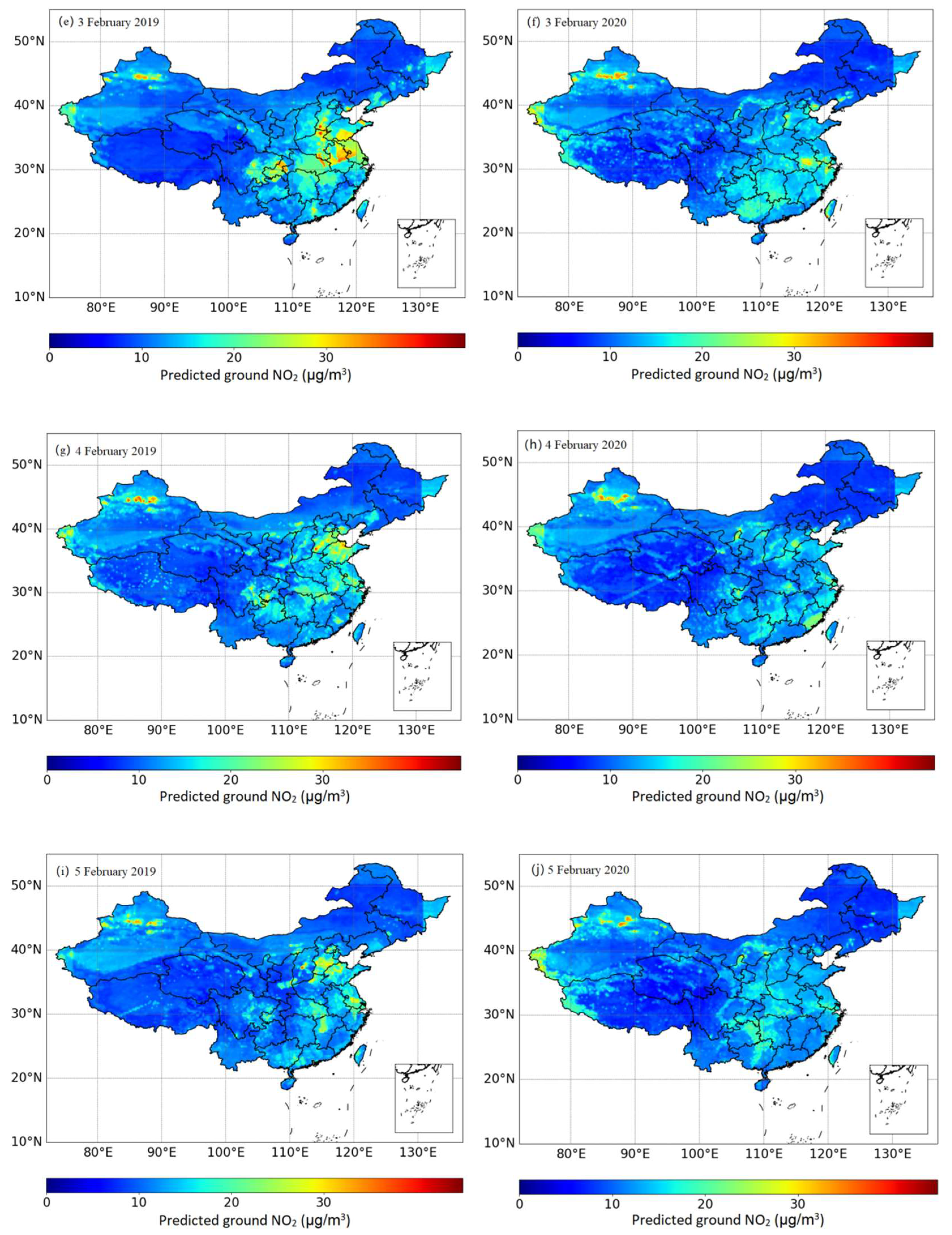
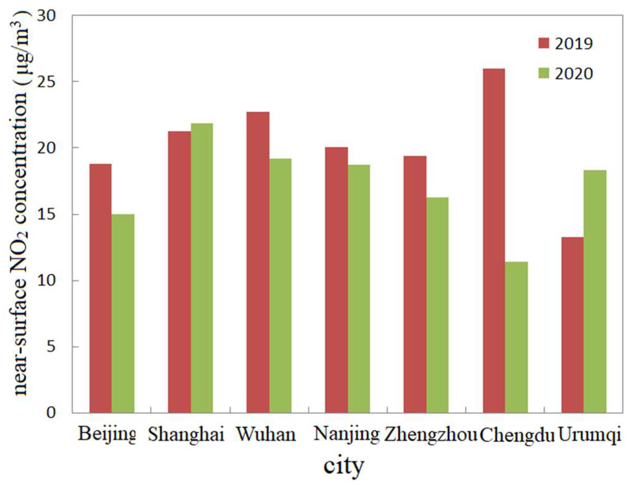
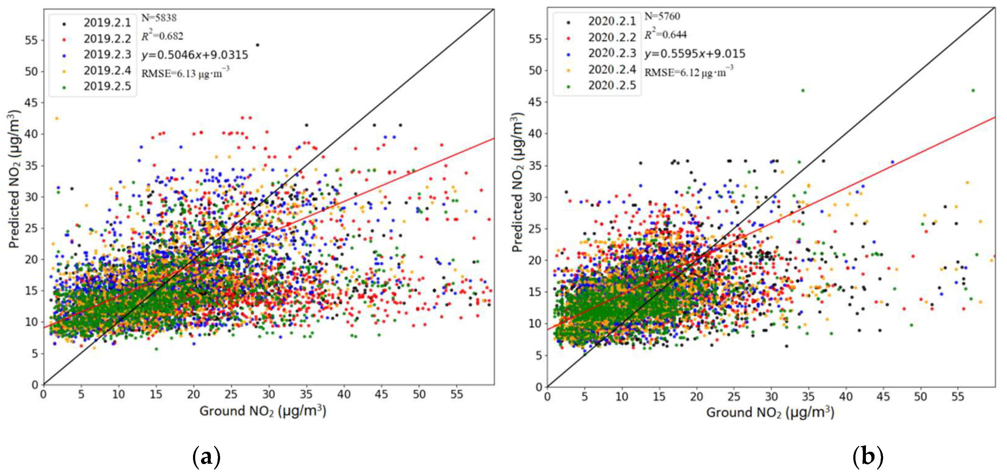
- The established model was used to estimate the near-surface NO2 concentration in China from 1–5 February 2020. Compared to the same period in 2019, it was found that the near-surface NO2 concentration in most parts of China decreased significantly in 2020, especially in the Beijing–Tianjin–Hebei region and Fenwei plain. This suggests that the strong measures taken by the Chinese government to control the COVID-19 pandemic have been well reflected by the forecast model, reflecting the practicability of the model forecast. From an analysis of seven typical cities, apart from Shanghai and Urumqi where the near-surface NO2 concentration in 2020 was slightly higher than that in 2019, other cities showed an obvious downward trend. By comparing and verifying the model-estimated results with the ground monitoring results, it was found that the results in 2019 and 2020 were basically the same. The R2 values reported were 0.682 and 0.644, and the RMSEs were 6.13 and 6.12 μg/m3, respectively. It further verifies that the model has good practicability in China.
Author Contributions
Funding
Data Availability Statement
Acknowledgments
Conflicts of Interest
References
- Logan, J.A. Nitrogen Oxides in the troposphere: Global and Regional Budgets. J. Geophys. Res. 1983, 88, 10785–10807. [Google Scholar] [CrossRef]
- Solomon, S.; Portmann, R.W.; Sanders, R.W.; Daniel, J.S.; Madsen, W.; Bartram, B.; Dutton, E.G. On The Role of Nitrogen Dioxide in the Absorption of Solar Radiation. J. Geophys. Res. 1999, 1041, 12047–12058. [Google Scholar] [CrossRef]
- Stavrakou, T.; MÜLler, J.F.; Boersma, K.F.; Van der, A.R.J.; Kurokawa, J.; Ohara, T.; Zhang, Q. Key Chemical NOx Sink Uncertainties and how They Influence Top-Down Emissions of Nitrogen Oxides. Atmos. Chem. Phys. 2013, 13, 7871–7929. [Google Scholar] [CrossRef] [Green Version]
- Crutzen, P.J. The Role of NO and NO2 in the Chemistry of the Troposphere and Stratosphere. Annu. Rev. Earth Planet. Sci. 1979, 7, 443–472. [Google Scholar] [CrossRef]
- Volz, A.; Kley, D. Evaluation of the Montsouris Series of Ozone Measurements Made in the Nineteenth Century. Nature 1988, 332, 240–242. [Google Scholar] [CrossRef]
- Barbara, J.; Finlayson-Pitts, J.N.; Pitts, J. CHAPTER 4—Photochemistry of Important Atmospheric Species. In Chemistry of the Upper and Lower Atmosphere; Elsevier: Amsterdam, The Netherlands, 2000; pp. 86–129. [Google Scholar]
- Duncan, B.N.; Lamsal, L.N.; Thompson, A.M.; Yoshida, Y.; Lu, Z.; Streets, D.G.; Hurwitz, M.M.; Pickering, K.E. A Space-Based, High-Resolution View of Notable Changes in Urban NOx Pollution around the World (2005–2014). J. Geophys. Res. Atmos. 2016, 121, 976–996. [Google Scholar] [CrossRef] [Green Version]
- Samoli, E. Short-Term Effects of Nitrogen Dioxide on Mortality: An Analysis within the APHEA Project. Eur. Respir. J. 2006, 27, 1129–1138. [Google Scholar] [CrossRef]
- Latza, U.; Gerdes, S.; Baur, X. Effects of Nitrogen Dioxide on Human Health: Systematic Review of Experimental and Epidemiological Studies Conducted between 2002 and 2006. Int. J. Hyg. Environ. Health 2009, 212, 271–287. [Google Scholar] [CrossRef] [PubMed]
- Chen, R.; Samoli, E.; Wong, C.M.; Huang, W.; Wang, Z.; Chen, B.; Kan, H. CAPES Collaborative Group. Associations between Short-Term Exposure to Nitrogen Dioxide and Mortality in 17 Chinese Cities: The China Air Pollution and Health Effects Study (CAPES). Environ. Int. 2012, 45, 32–38. [Google Scholar] [CrossRef]
- Zhang, R.; Li, Q.; Zhang, R. Meteorological Conditions for the Persistent Severe Fog and Haze Event over Eastern China in January 2013. Sci. China Earth Sci. 2014, 44, 26–35. [Google Scholar]
- Leue, C.; Wenig, M.; Wagner, T.; Klimm, O.; Platt, U.; Jhne, B. Quantitative Analysis of NOx Emissions from Global Ozone Monitoring Experiment Satellite Image Sequences. J. Geophys. Res. Atmos. 2001, 106, 5493–5505. [Google Scholar] [CrossRef] [Green Version]
- Shi, C.E.; Zhang, B.N. Tropospheric NO2 Columns over Northeastern North America: Comparison of CMAQ Model Simulations with GOME Satellite Measurements. Adv. Atmos. Sci. 2008, 1, 59–71. [Google Scholar] [CrossRef]
- Lamsal, L.N.; Duncan, B.N.; Yoshida, Y.; Krotkov, N.A.; Pickering, K.E.; Streets, D.G.; Lu, Z.U.S. NO2 Trends (2005–2013): EPA Air Quality System (AQS) Data versus Improved Observations from the Ozone Monitoring Instrument (OMI). Atmos. Environ. 2015, 110, 130–143. [Google Scholar] [CrossRef]
- Lamsal, L.N.; Martin, R.V.; Van Donkelaar, A.D.; Steinbacher, M.; Celarier, E.A.; Bucsela, E.; Dunlea, E.J.; Pinto, J.P. Ground-Level Nitrogen Dioxide Concentrations Inferred from the Satellite-Borne Ozone Monitoring Instrument. J. Geophys. Res. Atmos. 2008, 113, 1–15. [Google Scholar] [CrossRef] [Green Version]
- Levelt, P.F.; Hilsenrath, E.; Leppelmeier, G.W.; Van Den Oord, G.H.J.; Bhartia, P.K.; Tamminen, J.; De Haan, J.F.; Veefkind, J.P. Science Objectives of the Ozone Monitoring Instrument. IEEE Trans. Geosci. Remote Sens. 2006, 44, 1199–1208. [Google Scholar] [CrossRef]
- Levelt, P.F.; Van Den Oord, G.H.J.; Dobber, M.R.; Malkki, A.; Visser, H.; De Vries, J.; Stammes, P.; Lundell, J.O.V.; Saari, H. The Ozone Monitoring Instrument. IEEE Trans. Geosci. Remote Sens. 2006, 44, 1093–1101. [Google Scholar] [CrossRef]
- Martin, R.V.; Parrish, D.D.; Ryerson, T.B.; Nicks, D.K., Jr.; Chance, K.; Kurosu, T.P.; Jacob, D.J.; Sturges, E.D.; Fried, A.; Wert, B.P. Evaluation of GOME Satellite Measurements of Tropospheric NO2 and HCHO Using Regional Data from Aircraft Campaigns in the Southeastern United States. J. Geophys. Res. Atmos. 2004, 109, D24307. [Google Scholar] [CrossRef]
- Bucsela, E.J.; Perring, A.E.; Cohen, R.C.; Boersma, K.F.; Celarier, E.A.; Gleason, J.F.; Wenig, M.O.; Bertram, T.H.; Wooldridge, P.J.; Dirksen, R. Comparison of Tropospheric NO2 from in Situ Aircraft Measurements with Near-Real-Time and Standard Product Data from OMI. J. Geophys. Res. Atmos. 2008, 113, D16S31. [Google Scholar] [CrossRef]
- Burrows, J.P.; Weber, M.; Buchwitz, M.; Rozanov, V.; Ladstätter-Weißenmayer, A.; Richter, A.; Debeek, R.; Hoogen, R.; Bramstedt, K.; Eichmann, K.; et al. The Global Ozone Monitoring Experiment (GOME): Mission Concept and First Scientific Results. J. Atmos. Sci. 1999, 56, 151–175. [Google Scholar] [CrossRef]
- Bovensmann, H.; Burrows, J.P.; Buchwitz, M.; Frerick, J.; Noël, S.; Rozanov, V.V.; Chance, K.V.; Goede, A.P.H. SCIAMACHY: Mission Objectives and Measurement Modes. J. Atmos. Sci. 1999, 56, 127–150. [Google Scholar] [CrossRef] [Green Version]
- Zhao, X.; Fioletov, V.; Alwarda, R.; Su, Y.; Griffin, D.; Weaver, D.; Strong, K.; Cede, A.; Hanisco, T.; Tiefengraber, M.; et al. Tropospheric and Surface Nitrogen Dioxide Changes in the Greater Toronto Area during the First Two Years of the COVID-19 Pandemic. Remote Sens. 2022, 14, 1625. [Google Scholar] [CrossRef]
- Zhang, Q.; Streets, D.G.; He, K.; Wang, Y.; Richter, A.; Burrows, J.P.; Uno, I.; Jang, C.J.; Chen, D.; Yao, Z.; et al. NOx Emission Trends for China, 1995–2004: The View from the Ground and the View from Space. J. Geophys. Res. Atmos. 2007, 112, D22306. [Google Scholar] [CrossRef] [Green Version]
- Petritoli, A.; Bonasoni, P.; Giovanelli, G.; Ravegnani, F.; Kostadinov, I.; Bortoli, D.; Weiss, A.; Schaub, D.; Richter, A.; Fortezza, F. First Comparison between Ground-Based and Satellite-Borne Measurements of Tropospheric Nitrogen Dioxide in the Po Basin. J. Geophys. Res. Atmos. 2004, 109, D15307. [Google Scholar] [CrossRef] [Green Version]
- OrdÓNez, C.; Richter, A.; Steinbacher, M.; Zellweger, C.; Prévot, A.S.H.; Ordónez, C.; Nü, B.; Burrows, J.P. Comparison of 7 Years of Satellite-Borne and Ground-Based Tropospheric NO2 Measurements around Milan, Italy. J. Geophys. Res. Atmos. 2006, 111, D05310. [Google Scholar] [CrossRef] [Green Version]
- Qin, K.; Rao, L.; Xu, J.; Bai, Y.; Zou, J.; Hao, N.; Li, S.; Yu, C. Estimating Ground Level NO2 Concentrations over Central-Eastern China Using A Satellite-Based Geographically and Temporally Weighted Regression Model. Remote Sens. 2017, 9, 950. [Google Scholar] [CrossRef] [Green Version]
- Liu, F.; Beirle, S.; Zhang, Q.; Dörner, S.; He, K.; Wagner, T. NOx Lifetimes and Emissions of Cities and Power Plants in Polluted Background Estimated by Satellite Observations. Atmos. Chem. Phys. 2015, 15, 24179–24215. [Google Scholar]
- Bechle, M.J.; Millet, D.B.; Marshall, J.D. Remote Sensing of Exposure to NO2: Satellite versus Ground-Based Measurement in a Large Urban Area. Atmos. Environ. 2013, 69, 345–353. [Google Scholar] [CrossRef]
- Kim, H.C.; Lee, S.-M.; Chai, T.; Ngan, F.; Pan, L.; Lee, P. A Conservative Downscaling of Satellite-Detected Chemical Compositions: NO2 Column Densities of OMI, GOME-2, and CMAQ. Remote Sens. 2018, 10, 1001. [Google Scholar] [CrossRef] [Green Version]
- Byun, D.W.; Ching, J. Science Algorithms of the EPA Models-3 Community Multi-Scale Air Quality (CMAQ) Modeling System; NERL: Research Triangle Park, NC, USA, 1999; p. 425. [Google Scholar]
- Ghahremanloo, M.; Lops, Y.; Choi, Y.; Yeganeh, B. Deep Learning Estimation of Daily Ground-Level NO2 Concentrations From Remote Sensing Data. J. Geophys. Res. Atmos. 2021, 126, e2021JD034925. [Google Scholar] [CrossRef]
- Chen, Z.Y.; Zhang, R.; Zhang, T.H.; Ou, C.Q.; Guo, Y. A Kriging-Calibrated Machine Learning Method for Estimating Daily Ground-Level NO2 in Mainland China. Sci. Total Environ. 2019, 690, 556–564. [Google Scholar] [CrossRef] [PubMed]
- Lee, H.J.; Koutrakis, P. Daily ambient NO2 concentration predictions using satellite ozone monitoring instrument NO2 data and land use regression. Environ. Sci. Technol. 2014, 48, 2305–2311. [Google Scholar]
- Maasakkers, J.D.; Boersma, K.F.; Williams, J.E.; Van Geffen, J.; Veefkind, J.P. Vital Improvements to the Retrieval of Tropospheric NO2 Columns from the Ozone Monitoring Instrument. In Proceedings of the EGU General Assembly Conference Abstracts, Vienna, Austria, 7–12 April 2013. [Google Scholar]
- Wang, C.; Wang, T.; Wang, P.; Rakitin, V.S. Comparison and Validation of TROPOMI and OMI NO2 Observations over China. Atmosphere 2020, 11, 636. [Google Scholar] [CrossRef]
- Wang, Y.; Wang, J.; Zhou, M.; Henze, C.D.K.; Wang, W.G. Inverse Modeling of SO2 and NOx; Emissions over China Using Multisensor Satellite Data Part 2: Downscaling Techniques for Air Quality Analysis and Forecasts. Atmos. Chem. Phys. 2020, 20, 6651–6670. [Google Scholar] [CrossRef]
- Theys, N.; Smedt, I.D.; Yu, H.; Danckaert, T.; Gent, J.V.; Hörmann, C.; Wagner, T.; Hede-lt, P.; Bauer, H.; Romahn, F. Sulfur Dioxide Retrievals from TROPOMI Onboard Sentinel-5 Precursor: Algorithm Theoretical Basis. Atmos. Meas. Tech. 2017, 10, 119–153. [Google Scholar] [CrossRef] [Green Version]
- Borsdorff, T.; Andrasec, J.; Joost, A.D.B.; Hu, H.; Aben, I.; Landgraf, J. Detection of Carbon Monoxide Pollution from Cities and Wildfires on Regional and Urban Scales: The Benefit of CO Column Retrievals from SCIAMACHY 2.3ΜM Measurements Under Cloudy Conditions. Atmos. Meas. Tech. 2018, 11, 2553–2565. [Google Scholar] [CrossRef] [Green Version]
- Van Geffen, J.H.G.M.; Boersma, K.F.; Van Roozendael, M.; Hendrick, F.; Mahieu, E.; Smed, I.D.; Sneep, M.; Veefkind, J.P. Improved Spectral Fitting of Nitrogen Dioxide from OMI in the 405–465 Nm Window. Atmos. Meas. Tech. 2015, 8, 1685–1699. [Google Scholar] [CrossRef] [Green Version]
- Torres, O.; Decae, R.; Veefkind, J.P.; de Leeuw, G. OMI Aerosol Retrieval Algorithm. In OMI Algorithm Theoretical Basis Docu-ment: Clouds, Aerosols, and Surface UV Irradiance, 3, Version 2, OMI-ATBD-03; Stammes, P., Ed.; NASA Goddard Space Flight Center: Greenbelt, MD, USA, 2002; pp. 47–71. [Google Scholar]
- Gu, J.; Chen, L.; Yu, C.; Li, S.; Tao, J.; Fan, M.; Xiong, X.; Wang, Z.; Shang, H.; Su, L. Ground-Level NO2 Concentrations over China Inferred from the Satellite OMI and CMAQ Model Simulations. Remote Sens. 2017, 9, 519. [Google Scholar] [CrossRef] [Green Version]
- Hunter, J.D. Matplotlib: A 2D Graphics Environment. Comput. Sci. Eng. 2007, 9, 90–95. [Google Scholar] [CrossRef]
- Waskom, M.L. Seaborn: Statistical Data Visualization. J. Open Source Softw. 2021, 6, 3021. [Google Scholar] [CrossRef]
- Bisong, E. Matplotlib and Seaborn. Building Machine Learning and Deep Learning Models on Google Cloud Platform; Apress: Berkeley, CA, USA, 2019; pp. 151–165. [Google Scholar]
- Pukelsheim, F. The Three Sigma Rule. Am. Stat. 1994, 48, 88–91. [Google Scholar]
- Breiman, L. Random Forests, Machine Learning 45. J. Clin. Microbiol. 2001, 2, 199–228. [Google Scholar]
- Wu, H.; Ying, W. Benchmarking Machine Learning Algorithms for Instantaneous Net Surface Shortwave Radiation Retrieval Usingremote Sensing Data. Remote Sens. 2019, 11, 2520. [Google Scholar] [CrossRef] [Green Version]
- Liaw, A.; Wiener, M. Classification and Regression by Random-Forest. R News 2002, 23, 18–22. [Google Scholar]
- Scornet, E. Random Forests and Kernel Methods. IEEE Trans. Inf. Theory 2016, 62, 1485–1500. [Google Scholar] [CrossRef] [Green Version]
- Lee, S.; Kim, J. Prediction of Nanofiltration and Reverse-Osmosis-Membrane Rejection of Organic Compounds Using Random Forest Model. J. Environ. Eng. 2020, 146, 04020127. [Google Scholar]
- Lee, Y.; Han, D.; Ahn, M.H.; Im, J.; Lee, S.J. Retrieval of Total Precipitable Water from Himawari-8 AHI Data: A Comparison of Random Forest, Extreme Gradient Boosting, and Deep Neural Network. Remote Sens. 2019, 11, 1741. [Google Scholar] [CrossRef] [Green Version]
- Jenkins, J.M.; Kowalski, M.; Alvarenga, E.F.S. Predictive Modelling of Water Losses Using Random Forests on Weather Covariates. Water Supply 2018, 18, 2180–2187. [Google Scholar]
- Ruan, C.; Dong, Y.; Huang, W.; Huang, L.; Ye, H.; Ma, H.; Guo, A.; Sun, R. Integrating Remote Sensing and Meteorological Data to Predict Wheat Stripe Rust. Remote Sens. 2022, 14, 1221. [Google Scholar] [CrossRef]
- Pedregosa, F.; Varoquaux, G.; Gramfort, A.; Michel, V.; Thirion, B.; Grisel, O.; Blondel, M.; Prettenhofer, P.; Weiss, R.; Dubourg, V.; et al. Scikit-learn: Machine Learning in Python. J. Mach. Learn. Res. 2011, 12, 2825–2830. [Google Scholar]
- Bressert, E. SciPy and NumPy: An Overview for Developers; O’Reilly Media, Inc.: Sebastopol, CA, USA, 2012. [Google Scholar]
- Buitinck, L.; Louppe, G.; Blondel, M.; Pedregosa, F.; Mueller, A.; Grisel, O.; Niculae, V.; Prettenhofer, P.; Gramfort, A.; Grobler, J.; et al. API Design for Machine Learning Software: Experiences from the Scikit-Learn Project. In Proceedings of the ECML PKDD Workshop: Languages for Data Mining and Machine Learning, Bristol, UK, 23–27 September 2013; pp. 108–122. [Google Scholar]
- Zhan, Y.; Luo, Y.; Deng, X.; Zhang, K.; Zhang, M.; Grieneisen, M.L.; Di, B. Satellite-Based Estimates of Daily NO2 Exposure in China Using Hybrid Random Forest and Spatiotemporal Kriging Model. Environ. Sci. Technol. 2018, 52, 4180–4189. [Google Scholar] [PubMed]


| TropOMI | OMI | GOME-2 | SCIAMACHY | |
|---|---|---|---|---|
| Wavelength range (nm) | 405–465 | 405–465 | 425–450 | 426.5–451.5 |
| Secondary trace gases | O3, H2Ovap, O2-O2, H2Olip | O3, H2Ovap, O2-O2, H2Olip | O3, H2Ovap, O2-O2 | O3, H2Ovap, O2-O2 |
| False absorber | Ring | Ring | Ring | Ring |
| Fitting method | Non-linear | Non-linear | Linear | Linear |
| Polynomial term number | 5 | 5 | 3 | 2 |
| Polarization calibration | No | No | No | Yes |
| Name | Unit | Abbreviation |
|---|---|---|
| Temperature at 2 m height | °C | T |
| Relative humidity at 2 m height | % | RH |
| U component of wind at 2 m height | m/s | Ugrd |
| V component of wind at 2 m height | m/s | Vgrd |
| Boundary layer height | m | PBLH |
| Normalized vegetation index | - | NDVI |
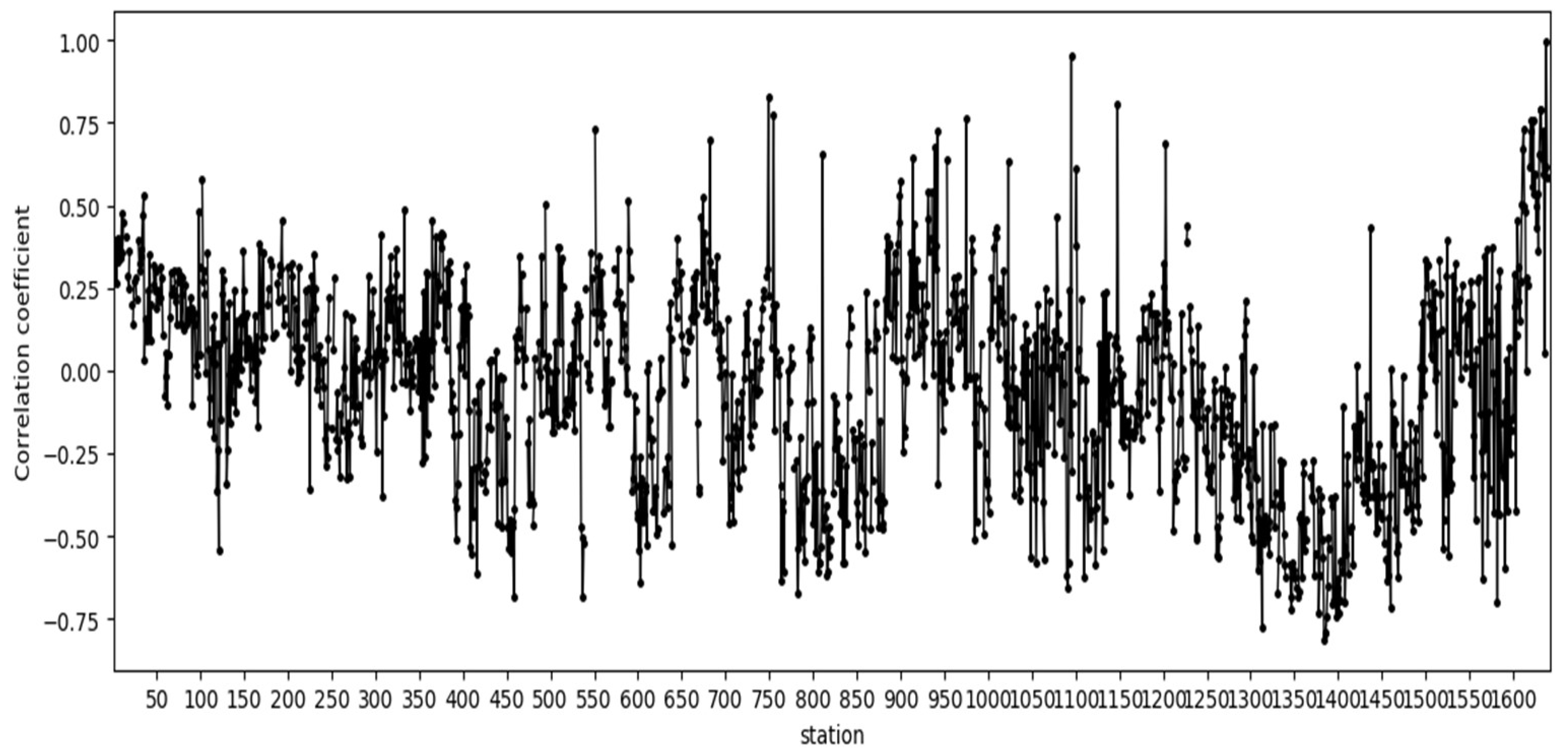
| Range | |r| > 0.7 | 0.5 ≤ |r| < 0.7 | 0.15 ≤ |r| < 0.5 | |r| < 0.15 | Nan |
|---|---|---|---|---|---|
| Number of sites | 28 | 134 | 801 | 545 | 133 |
| Maximum (mol/cm2) | Average (mol/cm2) | Median (mol/cm2) | |
|---|---|---|---|
| Near-real-time | 40.529 | 1.168 | 1.031 |
| Offline | 39.715 | 1.012 | 0.875 |
| Number of Samples | R2 | RMSE (μg/m3) | MSE (μg/m3) | MAE (μg/m3) | Interpretation Degree | |
|---|---|---|---|---|---|---|
| Training set | 5969 | 0.94 | 3.59 | 12.90 | 2.21 | 0.94 |
| Test set | 1990 | 0.78 | 7.04 | 49.54 | 5.00 | 0.78 |
Publisher’s Note: MDPI stays neutral with regard to jurisdictional claims in published maps and institutional affiliations. |
© 2022 by the authors. Licensee MDPI, Basel, Switzerland. This article is an open access article distributed under the terms and conditions of the Creative Commons Attribution (CC BY) license (https://creativecommons.org/licenses/by/4.0/).
Share and Cite
Li, M.; Wu, Y.; Bao, Y.; Liu, B.; Petropoulos, G.P. Near-Surface NO2 Concentration Estimation by Random Forest Modeling and Sentinel-5P and Ancillary Data. Remote Sens. 2022, 14, 3612. https://doi.org/10.3390/rs14153612
Li M, Wu Y, Bao Y, Liu B, Petropoulos GP. Near-Surface NO2 Concentration Estimation by Random Forest Modeling and Sentinel-5P and Ancillary Data. Remote Sensing. 2022; 14(15):3612. https://doi.org/10.3390/rs14153612
Chicago/Turabian StyleLi, Meixin, Ying Wu, Yansong Bao, Bofan Liu, and George P. Petropoulos. 2022. "Near-Surface NO2 Concentration Estimation by Random Forest Modeling and Sentinel-5P and Ancillary Data" Remote Sensing 14, no. 15: 3612. https://doi.org/10.3390/rs14153612