Multi-Dimensional Parameter Estimation in Polarimetric ULA with Cross-Distribution Dipole Pairs

Abstract

This paper investigates the estimation of parameters—including the elevation angle, azimuth angle, polarization auxiliary angle, polarization phase difference, frequency and range of near-field sources in a Polarimetric Uniform Linear Array (P-ULA) with defective electromagnetic vector sensors. The cross-distribution dipole pairs are alternately placed in the xoy plane and yoz plane, respectively, and the whole array is divided into two subarrays, where subarray 1 consists of all of the dipole pairs placed in the xoy plane, while the dipole pairs placed in yoz plane are gathered in subarray 2. Specifically, the polarization auxiliary angle and the polarization phase difference, as well as the elevation and azimuth angles of the sources, are firstly estimated based on the Fourth-Order Cumulant (FOC) matrix in each subarray. Moreover, a decoupling method is developed to obtain the elevation and azimuth. Subsequently, the frequency and range are estimated based on the FOC matrix. Then, the parameter pair matching method is performed in order to match the pairs. Finally, an analysis of the Cramér-Rao Bound (CRB) is provided, and comparisons of the root mean square error with respect to the different input signal-to-noise ratios and number of snapshots, among different estimation methods, are implemented in the environment of additive white gaussian noise. The simulation results are provided in order to verify the effectiveness and feasibility of the proposed method for multi-dimensional parameter estimation.

1. Introduction

Point-like source parameter estimation is one of the most important techniques in the array signal processing community, and it has been widely used in radar, seismic exploration, sonar, and many other fields [1,2,3,4,5]. A large number of methods has been developed to estimate parameters, especially in array radars [6,7,8,9]. In [10], a two-dimensional (2D) multiple-signal classification (MUSIC) method was proposed to estimate the azimuth and elevation angles of a planar array. However, there were disadvantageous that it suffered from the high computational load due to a 2D spectral peak searching. In [11], a two-stage MUSIC algorithm on a fourth-order cumulant (FOC) was developed in order to estimate spatial angles and localize mixed sources. At the expense of tremendous data samples, two-dimensional search and pairing parameters were avoided by the resultant algorithm, in addition, the estimation failure problem and alleviated aperture loss did not happen. Besides this, a method was developed by combining the estimation of the signal parameters via the rotational invariance techniques (ESPRIT) method and an FOC matrix in [12], where multi-dimensional parameter pair matching can be realized via the construction of the high-dimensional FOC matrix. The direction-of-arrival (DOA) of a nonuniform nested array was studied in [13], where the gain-phase error estimation was obtained by properly choosing the elements of the FOC matrix. In [14], several special FOC matrices were constructed to investigate the problem of mixed-source localization using a linear electromagnetic vector sensor (EVS) array with gain/phase uncertainties. Compared to the existing methods, it provided a satisfactory parameter estimation performance under unknown phase/gain responses, and does not impose a restriction on EVS placement. In order to localize mixed sources, several special FOC matrices were also constructed using a linear tripole (i.e., defective EVS (D-EVS)) array in [15]. It estimated both the spatial and polarization information of mixed sources; it provided improved accuracy without any spectral search, and realized a more reasonable classification of the signal types. These methods developed for spatial and polarization angle estimation are based on the FOC matrix; it is useful for the achievement of the 3-D localization of near-field (NF) sources, as well as the accurate estimation of the spatial and polarization parameters.

Moreover, the signal processing in a polarimetric array is an important topic in the electric and magnetic fields, where the polarimetric information can improve the performance of radar estimation [16,17,18]. The polarimetric array consists of EVS or D-EVS, where the D-EVS have more freedom in the spatial and polarization domains, and the mutual coupling among sensors is reduced. Besides this, the polarimetric information of D-EVS can also be utilized fully, and the computational load can be decreased to a greater degree than that for EVS. In [19], an improved method to estimate DOA and polarization angles was proposed based on D-EVS, where the polarimetric scale size and the computational complexity can be effectively decreased. The estimation of the DOA and polarization angles with a sparse collocated loop and dipole cross array was studied in [20], in which the ambiguities were resolved by the virtual baseline method, and the DOA estimation was acquired with high precision. In [21], a rapid DOA estimation method was developed based on the sparsely stretched L-shaped array with D-EVS, where the element spacing was greater than half the wavelength, and array aperture was effectively improved. Based on the a second-order statistics, two methods have proposed to estimate parameters of NF polarized sources using D-EVS array, where a sparse linear array was employed in [22] and an array of cross-dipoles was studied in [23]. A spatial amplitude ratio based algorithm and a noncircularity based algorithm were presented in [24,25], respectively, and effective for 2D NF polarized sources localization by utilizing the linear cocentered orthogonal loop and dipole array. While above methods in [19,20,21,22,23,24,25] are only effective for 1D DOA of uniform linear array (ULA) or 2D DOA of L-shaped/planar array sources localization, and fail to work 2D DOA estimation of ULA sources scenario.

Based on the above analysis, a novel polarimetric array with D-EVS is presented in this paper for multi-dimensional parameter estimation in a polarimetric ULA (P-ULA) with cross-distribution dipole pairs. In order to estimate the parameters, including the elevation angle, azimuth angle, polarization auxiliary angle, polarization phase difference, frequency and range of the NF sources, methods were designed as follows: Firstly, the polarization auxiliary angle and polarization phase difference, as well as the elevation angle and azimuth angle, are estimated based on the construction of the FOC matrix. Then, a decoupling method is developed to obtain the azimuth and elevation angles using the fixed phase difference in the spatial and polarization domains among the different subarrays. Subsequently, the frequency and range are estimated by re-applying the FOC matrix in each subarray. The parameter pair matching method is performed in order to match the pairs.

At the analysis stage, the Cramér-Rao Bound (CRB) for the elevation angle, azimuth angle, polarization auxiliary angle, polarization phase difference, frequency and range estimations are derived. Moreover, in order to investigate the performance of the proposed method, the root mean square error (RMSE) versus the input signal-to-noise ratio (SNR) and snapshots are analyzed in the environment of additive white gaussian noise (AWGN). In addition, comparisons between the proposed method, a method of multiple-input multiple-output radar using the electromagnetic vector sensors (EVS-MIMO) [26], are also given.

The paper is organized as follows. Section 2 presents the signal model of the P-ULA with cross-distribution dipole pairs. In Section 3, the problem of multi-dimensional parameter estimation is formulated and the methods to estimate the multi-dimensional parameters are introduced. The simulation experiment results are given in Section 4, and the performance discussion is addressed in Section 5. Finally, conclusions and possible future research are discussed in Section 6.

Regarding notation, boldface is used for vectors $\mathit{X}$ (upper case) whose $p-\mathrm{th}$ entry is $x\left(p\right)$, vectors $N$ (upper case) whose $p-\mathrm{th}$ entry is $n\left(p\right)$, vectors $S$ (upper case) whose $k-\mathrm{th}$ entry is $s_k$, and matrices $A$ (upper case) whose $(p,k)-\mathrm{th}$ entry is $a\left(p,k\right)$, $p=0,\cdots ,P-1$. The transpose, the conjugate, and the conjugate transpose operators are denoted by the symbols ${(\cdot )}^{\mathrm{T}}$, ${(\cdot )}^{*}$ and ${(\cdot )}^{\mathrm{H}}$, respectively. The $\odot$ and $\otimes$ represent the Hadamard (element-wise) product and the Kronecker product, respectively. The $\left[a,b\right]$ indicates a closed interval of $ℝ$ with $x\in {ℂ}^{P\times K}$, $\Vert x\Vert$ denotes its Euclidian norm. For any complex number $z$, $\left|z\right|$ are used to denote the modulus of $z$. Finally, $diag\left(x\right)$ indicates the diagonal matrix whose $i-\mathrm{th}$ diagonal element is the $i-\mathrm{th}$ entry of $x$. The ${[\cdot ]}_n$ represents the $n-\mathrm{th}$ diagonal element of a matrix. $I$, $0$ and $1$ denote, respectively, the identity matrix, the matrix with zero entries, and the vector with all elements being one (their size is determined from the context).

2. Received Signal Model

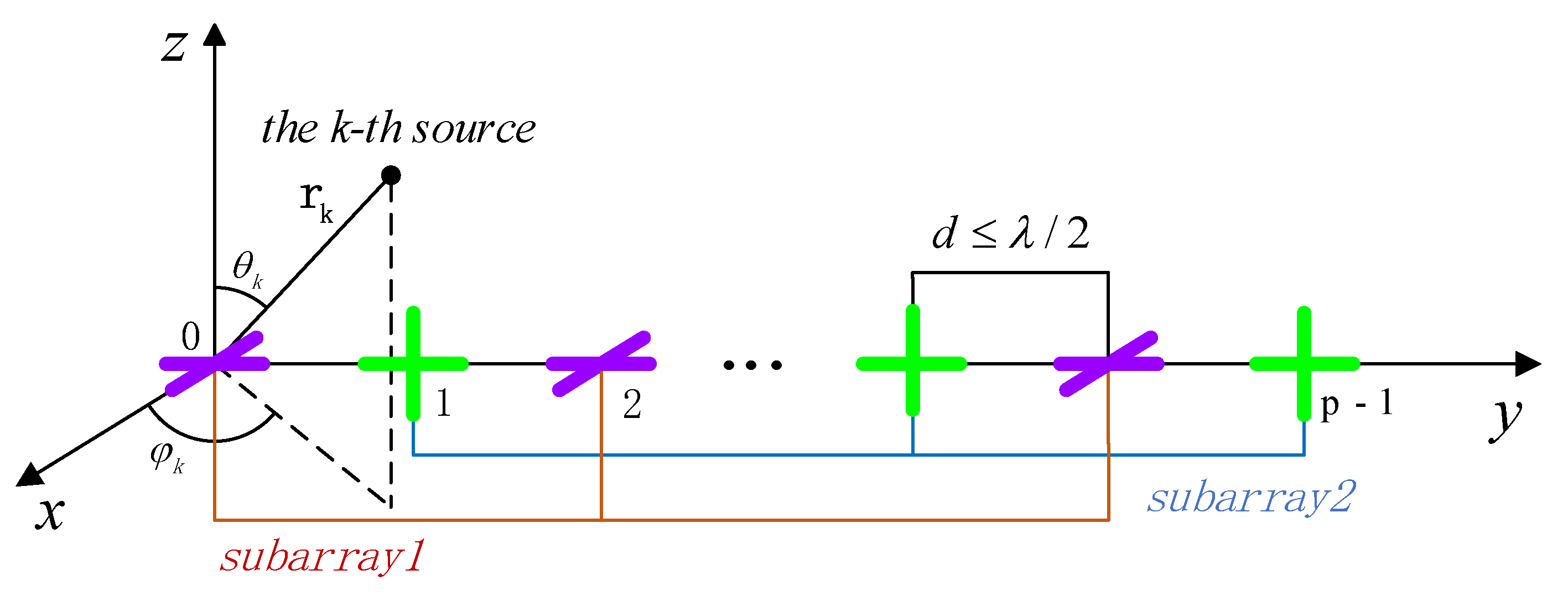
As shown in Figure 1, for the NF scenario in P-ULA with cross-distribution dipole pairs, let us assume a P-ULA with $P$ dipole pairs, where each dipole pair is composed of two identical electrically short dipoles which are orthogonally oriented. Furthermore, all of the dipole pairs are located in the y-axis with the spacing $d$, and the cross-distributed dipole pairs are alternately placed in the xoy plane and the yoz plane, respectively. To this end, the P-ULA with cross-distribution dipole pairs is divided into two subarrays, where subarray 1 consists of all of the dipole pairs placed in the xoy plane, while the dipole pairs placed in the yoz plane are gathered in subarray 2.

Consider $K$ NF independent signal sources, where the elevation angle, azimuth angle, polarization auxiliary angle and polarization phase difference of the $k-\mathrm{th}$ $\left(k=1,2,\cdots ,K\right)$ source are represented as ${\theta }_k$, ${\phi }_k$, ${\gamma }_k$, and ${\eta }_k$, respectively, with ${\theta }_k\in \left[0,\pi /2\right]$, ${\phi }_k\in \left[-\pi ,\pi \right]$, ${\gamma }_k\in \left[0,\pi /2\right]$, and ${\eta }_k\in \left[-\pi ,\pi \right]$, respectively. Besides this, the frequency and range of the $k-\mathrm{th}$ source are denoted as $f_k$ and $r_k$, respectively. Then, the received signal model can be derived as

$$X=AS+N$$

(1)

where $X\in {ℂ}^{\left(4P\times 1\right)}$ denotes the received signal matrix, $A={\left[A_1,A_2\right]}^{\mathrm{T}}\in {ℂ}^{\left(4P\times K\right)}$ represents the steering vector, and $A_1$ and $A_2$ are the steering vectors of subarray 1 and subarray 2, respectively, which has the form of

$$A_i=\left[a_{i,1},\cdots ,a_{i,K}\right],i=1,2$$

(2)

$S={\left[s_1,\cdots ,s_K\right]}^{\mathrm{T}}\in {ℂ}^{\left(K\times 1\right)}$ denotes the signal waveform matrix, and $N\in {ℂ}^{\left(4P\times 1\right)}$ represents AGWN. In particular, the signal received in the $p-\mathrm{th}$ dipole pairs is written as

$$x_{p,k}=a_{p,k}{s}_k+n_{p,k}$$

(3)

where $s_k=\beta e^{j2\pi f_{k}t}$ is the $k-\mathrm{th}$ signal with the complex echo amplitude $\beta$, $x_{p,k}$ denotes the $k-\mathrm{th}$ received signal, and $a_{1,k},a_{2,k}\in {ℂ}^{2P\times 1}$ indicates the steering vectors of $k-\mathrm{th}$ source, which can be represented as

$$a_{1,k}=q_k\otimes c_{1,k}\left({\theta }_k,{\phi }_k,{\gamma }_k,{\eta }_k\right)$$

$$a_{2,k}=q_k\otimes c_{2,k}\left({\theta }_k,{\phi }_k,{\gamma }_k,{\eta }_k\right)$$

(4)

where $q_k=\left[1,{\alpha }_{1,k},\cdots ,{\alpha }_{P-1,k}\right]$ with ${\alpha }_k=e^{j{\tau }_{p,k}}$, ${\tau }_{p,k}=d{\mu }_k+d^2{\varphi }_k$ represents the propagation delay of the $k-\mathrm{th}$ source with ${\mu }_k=-{\left(2\pi \sin {\theta }_k\sin {\phi }_k\right)/\lambda }_k$, ${\varphi }_k=\pi \left(1-{\sin }^2{\theta }_k{\sin }^2{\phi }_k\right)/{\lambda }_k{r}_k$, and the wavelength ${\lambda }_k\approx \lambda$.

Moreover, the electrical field component induced by the $p-\mathrm{th}$ dipole pairs is

$$c_{1,k}\left({\theta }_k,{\phi }_k,{\gamma }_k,{\eta }_k\right)={\left[e_{1,k},h\right]}^{\mathrm{T}}=F_{1,k}\left({\theta }_k,{\phi }_k\right)g\left({\gamma }_k,{\eta }_k\right)$$

$$c_{2,k}\left({\theta }_k,{\phi }_k,{\gamma }_k,{\eta }_k\right)={\left[e_{2,k},h\right]}^{\mathrm{T}}=F_{2,k}\left({\theta }_k,{\phi }_k\right)g\left({\gamma }_k,{\eta }_k\right)$$

(5)

where $F_{1,k}\left({\theta }_k,{\phi }_k\right)\in {ℂ}^{2\times 2}$ and $F_{2,k}\left({\theta }_k,{\phi }_k\right)\in {ℂ}^{2\times 2}$ represent the spatial angular location matrices of the $k-\mathrm{th}$ signal for subarray 1 and subarray 2, respectively, which are written respectively as

$$F_{1,k}\left({\theta }_k,{\phi }_k\right)=\left[\begin{array}{cc}\cos \theta \cos \phi & -\sin \phi \\ \cos \theta \sin \phi & \cos \phi \end{array}\right]$$

$$F_{2,k}\left({\theta }_k,{\phi }_k\right)=\left[\begin{array}{cc}\cos \theta \sin \phi & \cos \phi \\ -\sin \theta & 0\end{array}\right]$$

(6)

$g\left({\gamma }_k,{\eta }_k\right)$ represents the $2\times 1$ vector of the polarization vector in each subarray, which is expressed as

$$g\left({\gamma }_k,{\eta }_k\right)=\left[\begin{array}{c}\sin \gamma e^{j\eta }\\ \cos \gamma \end{array}\right]$$

(7)

Note that some assumptions in this paper are listed as follows. The source signals are statistically independent as zero-mean random processes with nonzero kurtosis distribution. $N\sim \left(0,Q\right)$ is AGWN with $Q\in {ℍ}^{4P}$ the positive definite covariance matrix. For different sources, the phase parameters are independent, i.e., ${\mu }_i\ne {\mu }_j$ and ${\varphi }_i\ne {\varphi }_j$ for $i\ne j$. The form of the received data in each vector sensor is the same, and the spacing of element $d\le \lambda /2$ and the number of sources $K\le P$ are known or accurately estimated by theoretical information criteria.

3. Joint Parameter Estimation Method

This section deals with the parameter estimation of the NF sources, including the elevation angle, azimuth angle, polarization auxiliary angle, polarization phase difference, frequency and range. Firstly, the elevation angle, azimuth angle, polarization auxiliary angle and polarization phase difference of the sources are estimated based on the FOC matrix in each subarray. Then, a decoupling method is developed to obtain the azimuth and elevation angles using the fixed phase difference in the spatial and polarization domains among the different subarrays. Subsequently, the frequency and range are estimated by re-applying the FOC matrix. Finally, the parameter pair matching method is performed in order to match the pairs.

3.1. Polarization Angle Estimation of the Subarray

Based on the principle of FOC [15] and the above assumptions, the cumulant matrix at the $p-\mathrm{th}$ dipole pair of each subarray can be defined as

$$C_i={\displaystyle \sum _{i=1,j=1}^{2}cum\left\{x_{p,k}^i,{\left(x_{q,k}^j\right)}^{*},X,X^{\mathrm{H}}\right\}}=A_i{R}_i{A}_i^{\mathrm{H}}$$

(8)

where $C={\left[C_{1p},C_{2p},C_{3q},C_{4q}\right]}^T$, $C_{1p}$ and $C_{2p}$ denote the $x$ and $y$ dipoles of the $p-\mathrm{th}$ dipole pairs in subarray 1, respectively, and $C_{3q}$ and $C_{4q}$ represent the $x$ and $y$ dipole of the $q-\mathrm{th}$ dipole pairs in subarray 1, respectively. $x_{p,k}^i=a_{p,k}^i{s}_k$ with $i$ denote $x$ dipole or $y$ dipole, and $j$ is the same, with $p,q=0,2,\cdots$ representing the location of the dipole pairs in subarray 1.

$$C={\left[C_p^{\mathrm{T}},C_q^{\mathrm{T}}\right]}^{\mathrm{T}}$$

(9)

$$R_i=diag\left\{{\displaystyle \sum _{k=1}^K{\displaystyle \sum _{i=1,j=1}^2\left(a_{p,k}^i,{\left(a_{q,k}^j\right)}^{*}\right)s_k}}\right\}$$

(10)

Then, the subspace theory can be implemented using the signal subspace matrix $E_S$, where the eigen-decomposition $R=E_s{\sigma }_s^2{E}_s^{\mathrm{H}}+E_n{\sigma }_n^2{E}_n^{\mathrm{H}}$ in (10), i.e.,

$$E_S={\left[{\left[A_1{R}_1\right]}^{\mathrm{T}},{\left[A_2{R}_2\right]}^{\mathrm{T}}\right]}^{\mathrm{T}}T$$

(11)

where $T\in {ℂ}^{K\times K}$ denotes an invertible matrix. Let us first consider the case without noise. Hence, a unique $K\times K$ non-singular matrix exists, such that $E_S=AT$. In particular, $E_S^{\left(i\right)}$ represents a block matrix of $E_S$ with elements from the $\left(2\left(i-1\right)P+1\right)-\mathrm{th}$ row to the $\left(2iP\right)-\mathrm{th}$ row. The $E_S^{\left(j\right)}$ is similar to $E_S^{\left(i\right)}$, and $i\ne j$. Consequently, the $E_S$ can be expressed as

$$E_S^{\left(i\right)}=J^{\left(i\right)}{E}_S=A_i{R}_{i}T$$

$$E_S^{\left(j\right)}=J^{\left(j\right)}{E}_S=A_j{R}_{j}T=A_i{R}_i{H}^{\left(i,j\right)}T$$

(12)

where $R_{j}T=R_i{H}^{\left(i,j\right)}T$, and $J^{\left(i\right)}=e_i\otimes I_P$ denotes a selection matrix with $e_i$, which is a $1\times 2$ row vector (where the $i-\mathrm{th}$ dipole is $1$ and the others are $0$ in $e_i$). Furthermore, as $E_S^{\left(j\right)}$ and $E_S^{\left(i\right)}$ are full-rank matrices, a unique non-singular $K\times K$ matrix $Q_S^{\left(i,j\right)}$ exists, such that

$$E_S^{\left(j\right)}=E_S^{\left(i\right)}{Q}_S^{\left(i,j\right)}\Rightarrow Q_S^{\left(i,j\right)}={\left({\left(E_S^{\left(i\right)}\right)}^{\mathrm{H}}{E}_S^{\left(i\right)}\right)}^{-1}{\left(E_S^{\left(i\right)}\right)}^{\mathrm{H}}{E}_S^{\left(j\right)}$$

(13)

Then, it follows that

$$A_i{R}_i{H}^{\left(i,j\right)}T=A_j{R}_{j}T{Q}_S^{\left(i,j\right)}\Rightarrow Q_S^{\left(i,j\right)}=T^{-1}{H}^{\left(i,j\right)}T$$

(14)

In (14), $H^{\left(i,j\right)}$ and $T$ indicate the eigenvalues and the right eigenvectors of $Q_S^{\left(i,j\right)}$, respectively. Note that the eigenvalues of $Q_S^{\left(i,j\right)}$ correspond to the diagonal elements of $H^{\left(i,j\right)}$, which has the form of

$$H^{\left(i,j\right)}=diag\left(\frac{e_{p-1,1}^j}{e_{p,1}^i},\cdots ,\frac{e_{p-1,K}^j}{e_{p,K}^i}\right)$$

(15)

where $e_{p-1,k}^j$ and $e_{p,k}^i$ denote the $j-\mathrm{th}$ row of $e_{p-1,k}$ and the $i-\mathrm{th}$ row of $e_{p,k}$, respectively.

Accordingly, the $k-\mathrm{th}$ source polarization auxiliary angle and polarization phase difference estimation at the $p-\mathrm{th}$ dipole pairs can be derived as

$$\sin {\widehat{\theta }}_k\sin {\widehat{\phi }}_k=-\frac{{\left[H^{\left(2,1\right)}\right]}_k}{{\left[H^{\left(1,1\right)}\right]}_k}$$

(16)

$${\widehat{\eta }}_{p,k}=\mathrm{angle}\left(\frac{-{\left[H^{\left(1,1\right)}\right]}_k\sin {\widehat{\phi }}_{p,k}}{\left|{\left[H^{\left(1,1\right)}\right]}_k\right|\cos {\widehat{\phi }}_{p,k}}\right)$$

(17)

$${\widehat{\gamma }}_{p,k}=\arctan \left(\frac{\cos {\widehat{\phi }}_{p,k}\sin {\widehat{\eta }}_{p,k}}{imag\left\{{\left[H^{\left(2,1\right)}\right]}_k\right\}\sin {\widehat{\theta }}_{p,k}}\right)$$

(18)

Similarly, the estimation of the $k-\mathrm{th}$ source polarization auxiliary angle and polarization phase difference at the $q-\mathrm{th}$ dipole pairs can be obtained, the FOC matrix is designed as follows:

$$C_i={\displaystyle \sum _{i=1,j=1}^{2}cum\left\{x_{q,k}^i,{\left(x_{p,k}^j\right)}^{*},X,X^{\mathrm{H}}\right\}}=A{V}_i{A}^{\mathrm{H}}$$

(19)

where $x_{q,k}^i=a_{q,k}^i{s}_k$ is similar to $x_{p,k}^i$, and

$$V_i=diag\left\{{\displaystyle \sum _{k=1}^K{\displaystyle \sum _{i=1,j=1}^2\left(a_{q,k}^i,{\left(a_{p,k}^j\right)}^{*}\right)s_k}}\right\}$$

(20)

Then, based on the subspace theory and the above procedure, the estimation of ${\widehat{\eta }}_{q,k}$ and ${\widehat{\gamma }}_{q,k}$ can be obtained at subarray 1. Refer to the above derivation process, polarization auxiliary angle and polarization phase difference estimation at $\left(p-1\right)-\mathrm{th}$, the $\left(q-1\right)-\mathrm{th}$ dipole pairs are ${\widehat{\eta }}_{p-1,k}$,${\widehat{\gamma }}_{p-1,k}$,${\widehat{\eta }}_{q-1,k}$ and ${\widehat{\gamma }}_{q-1,k}$ of the $k-\mathrm{th}$ source at subarray 2.

As a consequence, the polarization auxiliary angle and polarization phase difference estimation at the P-ULA with cross-distribution dipole pairs can be given by

$${\widehat{\eta }}_k=\left({\widehat{\eta }}_{p,k}+{\widehat{\eta }}_{q,k}+{\widehat{\eta }}_{p-1,k}+{\widehat{\eta }}_{q-1,k}\right)/4$$

(21)

$${\widehat{\gamma }}_k=\left({\widehat{\gamma }}_{p,k}+{\widehat{\gamma }}_{q,k}+{\widehat{\gamma }}_{p-1,k}+{\widehat{\gamma }}_{q-1,k}\right)/4$$

(22)

By constructing the FOC matrix, the estimation of ${\widehat{\gamma }}_k$, ${\widehat{\eta }}_k$ and $\sin {\widehat{\theta }}_k\sin {\widehat{\phi }}_k$ can be derived. Moreover, the estimations of the subarray procedure are synthetically reported (Algorithm 1).

Algorithm 1: Polarization angle estimation of the subarray procedure.

Input:${\theta }_k$,${\phi }_k$,${\gamma }_k$,${\eta }_k$,$A$,$S$,$N$. Output: A solution to$\sin {\widehat{\theta }}_k\sin {\widehat{\phi }}_k$, ${\widehat{\gamma }}_k$, ${\widehat{\eta }}_k$.  Initialization: $n=0$, ${\widehat{\theta }}_{p,k}={\theta }_k$, ${\widehat{\phi }}_{p,k}={\phi }_k$, ${\widehat{\gamma }}_{p,k}={\gamma }_k$, ${\widehat{\eta }}_{p,k}={\eta }_k$.  repeat (optimization for initial search parameter given by ${\gamma }_k$, ${\eta }_k$). 1. Construct $C_i$ using (8); 2. Compute $E_S^{\left(i\right)}$, $E_S^{\left(j\right)}$ and $H^{\left(i,j\right)}$ using (12)–(15); 3. Evaluate $\sin {\widehat{\theta }}_k\sin {\widehat{\phi }}_k$, ${\widehat{\gamma }}_k$, ${\widehat{\eta }}_k$ using (16)–(18); 4. Repeat 1–3, evaluate for subarray 2; 5. Determine ${\widehat{\gamma }}_k$, ${\widehat{\eta }}_k$ using (21)–(22).

3.2. Decoupling Method of the Elevation and Azimuth

In this subsection, the mutual coupling effect across the P-ULA with cross-distribution dipole pairs is considered, and a decoupling method of the elevation and azimuth is developed in order to further improve the parameter estimation accuracy. The mutual coupling effect of the existing collocated vector sensor array contains two parts, among the elements and between the internal polarization antennas of collocated dipole pairs. The mutual coupling effect emerges when the element spacing $d=\lambda /2$. As shown in Figure 1, the polarization antennas of subarray 1 are x-1 and y-1, and those of subarray 2 are y-2 and z-2. The mutual coupling effect of the spatial field and polarization field is produced by x-1 and y-2, x-1 and z-2, and y-1 and z-2. The mutual coupling effect of the spatial field appears by y-1 and y-2. For the internal polarization antennas of collocated dipole pairs, the mutual coupling effect of the polarization field arises by x-1 and y-1, and y-2 and z-2. The array’s scalability is decreased, complexity and computation of the parameter estimation algorithm are increased due to the mutual coupling effect of the array. Thus, a decoupling method is a significant step in parameter estimation.

Consider that $\sin {\widehat{\theta }}_k\sin {\widehat{\phi }}_k$ is included in propagation delay ${\widehat{\tau }}_{p,k}$ and ${\widehat{\tau }}_{p-1,k}$. The elevation angle and azimuth angle can only be estimated in quadrant 1/2 or 3/4, and they generate a set of cyclical coupling [27]. In Figure 1, $A$ is the array manifold matrix, $a_{p,k}^x$ is the x-axis dipole of subarray 1, $a_{p,k}^y$ is the y-axis dipole of subarray 1, $a_{p-1,k}^z$ is the z-axis dipole of subarray 2, and $a_{p-1,k}^y$ is the y-axis dipole of subarray 2.

According to the principle of the ESPRIT algorithm [28], there is a fixed phase difference among the different subarrays, which can be expressed as

$$a_{p,k}^x=a_{p-1,k}^z\Sigma$$

$$a_{p-1,k}^y=a_{p-1,k}^z\Xi$$

(23)

where $\mathsf{\Sigma }$ represents the phase difference of the spatial field and polarization field between the x-axis dipole of subarray 1 and the z-axis dipole of subarray 2. $\Xi$ denotes the phase difference of the polarization field between the y-axis dipole and the z-axis dipole of subarray 2.

$$\Sigma =diag\left[\begin{array}{cc}\frac{e_{p,1}^x}{e_{p-1,1}^z}{\tau }_{p,1}& \begin{array}{cc}\frac{e_{p,2}^x}{e_{p-1,2}^z}{\tau }_{p,2}& \begin{array}{cc}\cdots & \frac{e_{p,K}^x}{e_{p-1,K}^z}{\tau }_{p,K}\end{array}\end{array}\end{array}\right]$$

$$\Xi =diag\left[\begin{array}{cc}\begin{array}{cc}\begin{array}{cc}\frac{e_{p-1,1}^y}{e_{p-1,1}^z}& \frac{e_{p-1,2}^y}{e_{p-1,2}^z}\end{array}& \cdots \end{array}& \frac{e_{p-1,K}^y}{e_{p-1,K}^z}\end{array}\right]$$

(24)

Elements on the diagonal are ${\tau }_{p,k}$, which represents the spatial phase difference of the $k-\mathrm{th}$ signal between the y-axis dipole of subarray 1 and the y-axis dipole of subarray 2. Diagonal elements can be represented as

$$\frac{e_{p,k}^x}{e_{p-1,k}^z}{\tau }_{p,k}=-\left(\frac{\cos {\phi }_k}{\tan {\theta }_k}-\frac{\sin {\phi }_k}{\sin {\theta }_k\tan {\gamma }_k{e}^{j{\eta }_k}}\right){\tau }_{p,k}={\Sigma }_k$$

$$\frac{e_{p-1,k}^y}{e_{p-1,k}^z}=-\left(\frac{\sin {\phi }_k}{\tan {\theta }_k}+\frac{\cos {\phi }_k}{\sin {\theta }_k\tan {\gamma }_k{e}^{j{\eta }_k}}\right)={\Xi }_k$$

(25)

In order to process Equation (25), $\tan {\phi }_k$ can be obtained as follows:

$$\tan {\phi }_k=-imag\left({\Sigma }_k/{\tau }_{p,k}\right)/imag\left({\Xi }_k\right)$$

(26)

In this case, ${\widehat{\phi }}_k\in \left[-\pi /2,\pi /2\right]$ needs to be decoupled in order to judge the quadrant of azimuth angle ${\phi }_k$ according to the positive or negative of $\sin {\theta }_k\sin {\phi }_k$, and $\tan {\phi }_k$. Then, ${\phi }_k$ is calculated and ${\theta }_k$ is determined. Therefore, discuss the following four assumptions.

Assumption 1, ${\phi }_k$ is in the first quadrant:

$$\{\begin{array}{c}\sin {\theta }_k\sin {\phi }_k>0\\ \tan {\phi }_k>0\end{array}\Rightarrow \{\begin{array}{c}{\theta }_k\in \left[0,\pi /2\right]\\ {\phi }_k\in \left[0,\pi /2\right]\end{array}$$

(27)

Assumption 2, ${\phi }_k$ is in the second quadrant:

$$\{\begin{array}{c}\sin {\theta }_k\sin {\phi }_k>0\\ \tan {\phi }_k<0\end{array}\Rightarrow \{\begin{array}{c}{\theta }_k\in \left[0,\pi /2\right]\\ {\phi }_k\in \left[\pi /2,\pi \right]\end{array}$$

(28)

Assumption 3, ${\phi }_k$ is in the third quadrant:

$$\{\begin{array}{c}\sin {\theta }_k\sin {\phi }_k<0\\ \tan {\phi }_k>0\end{array}\Rightarrow \{\begin{array}{c}{\theta }_k\in \left[0,\pi /2\right]\\ {\phi }_k\in \left[-\pi ,-\pi /2\right]\end{array}$$

(29)

Assumption 4, ${\phi }_k$ is in the fourth quadrant:

$$\{\begin{array}{c}\sin {\theta }_k\sin {\phi }_k<0\\ \tan {\phi }_k<0\end{array}\Rightarrow \{\begin{array}{c}{\theta }_k\in \left[0,\pi /2\right]\\ {\phi }_k\in \left[-\pi /2,0\right]\end{array}$$

(30)

As a consequence, the elevation angle and azimuth angle estimation are given as follows:

$${\widehat{\phi }}_k=\arctan \left[-imag\left({\widehat{\Sigma }}_k/{\tau }_{p,k}\right)/imag\left({\widehat{\Xi }}_k\right)\right]$$

(31)

$${\widehat{\theta }}_k=\arcsin \frac{\left(\sqrt{\pi \left(d^2+{\widehat{r}}_k^2\right)+\mathrm{angle}\left({\tau }_{p,k}\right)\lambda {\widehat{r}}_k}-\sqrt{\pi }{\widehat{r}}_k\right)}{\left(\sqrt{\pi }\sin {\widehat{\phi }}_k\right)}$$

(32)

The source angles can be estimated by two diagonal matrices, $\mathsf{\Sigma }$ and $\Xi$.

Hence, refer to the derivation process of the decoupling method, the NF source angles estimation of the subarray are obtained as ${\widehat{\phi }}_{p,k}$, ${\widehat{\phi }}_{p-1,k}$, ${\widehat{\theta }}_{p,k}$ and ${\widehat{\theta }}_{p-1,k}$. Therefore, the elevation and azimuth angles estimation of the NF sources can be given by

$${\widehat{\phi }}_k=\left({\widehat{\phi }}_{p,k}+{\widehat{\phi }}_{p-1,k}\right)/2$$

(33)

$${\widehat{\theta }}_k=\left({\widehat{\theta }}_{p,k}+{\widehat{\theta }}_{p-1,k}\right)/2$$

(34)

According to Section 3.1, $\sin {\widehat{\theta }}_k\sin {\widehat{\phi }}_k$ generated a set of cyclical coupling in the elevation angle and azimuth angle. While in this subsection, the decoupling method of the elevation and azimuth angles is applied to obtain ${\widehat{\theta }}_k$ and ${\widehat{\phi }}_k$. The estimation steps in the decoupling method are shown as follows (Algorithm 2).

Algorithm 2: Decoupling of elevation and azimuth angles.

Input:${\theta }_k$,${\phi }_k$,$a_{p,k}^i$,${\tau }_{p,k}$. Output: A solution to${\widehat{\theta }}_k$,${\widehat{\phi }}_k$.  Initialization: $n=0$, ${\widehat{\theta }}_{p,k}={\theta }_k$, ${\widehat{\phi }}_{p,k}={\phi }_k$.  repeat (optimization for initial search parameter given by ${\theta }_k$, ${\phi }_k$). 1. Obtain the fixed phase difference between different subarrays using (23)–(24); 2. Compute two diagonal matrices $\Sigma$ and $\Xi$ using (25); 3. Judge quadrant of azimuth angle, then determine elevation angle; 4. Evaluate ${\widehat{\theta }}_k$, ${\widehat{\phi }}_k$ using (31)–(34).

3.3. Estimation Frequency and Range of Sources

Based on the received signal model and the FOC matrix, the following cumulant of subarray 1 can be constructed:

$$C_i={\displaystyle \sum _{i=1,j=1}^{2}cum\left\{{\left(x_{p,k}^i\right)}^{*},x_{p,k}^j,{\left(x_{q,k}^j\right)}^{*},x_{q,k}^i\right\}}$$

(35)

where $C={\left[C_{1p},C_{2p},C_{3q},C_{4q}\right]}^{\mathrm{T}}$, $x_{p,k}^i$ and $x_{q,k}^j$ are similar to Section 3.1, and the FOC matrices include

$$C_{1p}=A_{p,k}{s}_k{A}_{p,k}^{\mathrm{H}}$$

$$C_{2p}=A_{p,k}{\Lambda }_p{s}_k{A}_{p,k}^{\mathrm{H}}$$

$$C_{3q}=A_{p,k}{\Omega }_p{s}_k{A}_{p,k}^{\mathrm{H}}$$

$$C_{4q}=A_{p,k}{\Phi }_p{s}_k{A}_{p,k}^{\mathrm{H}}$$

(36)

where $C_{1p},C_{2p},C_{3q},C_{4q}\in {ℂ}^{P\times P}$, and the FOC matrix is a full-rank matrix. Compute the rotation invariant matrices ${\Lambda }_p$, ${\Omega }_p$ and ${\Phi }_p$ as follows:

$${\Lambda }_p=diag\left\{\begin{array}{ccc}{e}^{j2\pi f_{p,1}}& \cdots & e^{j2\pi f_{p,K}}\end{array}\right\}$$

$${\Omega }_p=diag\left\{\begin{array}{ccc}{e}^{j4{\mu }_{p,1}}& \cdots & e^{j4{\mu }_{p,K}}\end{array}\right\}$$

$${\Phi }_p=diag\left\{\begin{array}{ccc}{e}^{-j8{\varphi }_{p,1}}& \cdots & e^{-j8{\varphi }_{p,K}}\end{array}\right\}$$

(37)

Hence, the relative of matrices can be defined as $E_1$, $E_2$ and $E_3$, where

$$E_1=C_2{C}_1^{\mathrm{H}}$$

$$E_2=C_3{C}_1^{\mathrm{H}}$$

$$E_3=C_4{C}_1^{\mathrm{H}}$$

(38)

Then, the relationship of the FOC matrices can be represented as

$$E_1{A}_{p,k}=A_{p,k}{\Lambda }_p$$

$$E_2{A}_{p,k}=A_{p,k}{\Omega }_p$$

$$E_3{A}_{p,k}=A_{p,k}{\Phi }_p$$

(39)

where the diagonal element ${\Lambda }_p$ is the eigenvalue of matrix $E_1$, and the $k-\mathrm{th}$ column vector $a_{p,k}$ of the array manifold $A_{p,k}$ is the eigenvector corresponding to the eigenvalue.

The eigen-decompositions of the matrices $E_1$, $E_2$ and $E_3$ are managed, then, eigenvalues are obtained, and parameters can be given. The rank order of $E_1$, $E_2$ and $E_3$ is different, while the eigenvectors of the matrices are the same. Therefore, it is necessary to know the pairing relationship among the feature vectors, and to estimate each parameter.

The eigenvector matrices are obtained by the eigen-decomposition, the eigenvalue matrices are ${\widehat{\Lambda }}_p$, ${\widehat{\Omega }}_p$ and ${\widehat{\Phi }}_p$. The pairing method is as follows: based on the matrix ${\widehat{A}}_{p,k}^{E_1}$, the constructed eigenvectors of the matrix ${\widehat{A}}_{p,k}^{E_2}$, ${\widehat{A}}_{p,k}^{E_3}$ are aligned with the matrix ${\widehat{A}}_{p,k}^{E_1}$, matching the corresponding eigenvalues one by one. The eigenvalues are ${\left[\Lambda \right]}_{p,k}$, ${\left[\Omega \right]}_{p,k}$ and ${\left[\Phi \right]}_{p,k}$, the eigenvectors are ${\widehat{A}}_{p,k}^{E_1}$, ${\widehat{A}}_{p,k}^{E_2}$ and ${\widehat{A}}_{p,k}^{E_3}$. The pairing of the eigenvalue matrices is realized as

$$P_1={\left({\left({\widehat{A}}_{p,k}^{E_2}\right)}^H{\widehat{A}}_{p,k}^{E_2}\right)}^{-1}{\left({\widehat{A}}_{p,k}^{E_2}\right)}^H{\widehat{A}}_{p,k}^{E_1}$$

$$P_2={\left({\left({\widehat{A}}_{p,k}^{E_3}\right)}^H{\widehat{A}}_{p,k}^{E_3}\right)}^{-1}{\left({\widehat{A}}_{p,k}^{E_3}\right)}^H{\widehat{A}}_{p,k}^{E_1}$$

(40)

The NF source parameter estimation of subarray 1 is derived as follows:

$${\widehat{f}}_{p,k}=-\frac{\mathrm{angle}\left({\left[\widehat{\Lambda }\right]}_{p,k}\right)}{2\pi }$$

(41)

$${\widehat{r}}_{p,k}=\frac{{\left(2\pi d\right)}^2-{\left({\left[\widehat{\Omega }\right]}_{p,k}\lambda \right)}^2}{4\pi \lambda {\left[\widehat{\Phi }\right]}_{p,k}}$$

(42)

Repeat the above steps, the cumulant of subarray 2 can be constructed as

$$C_i={\displaystyle \sum _{i=1,j=1}^{2}cum\left\{{\left(x_{p-1,k}^i\right)}^{*},x_{p-1,k}^j,{\left(x_{q-1,k}^j\right)}^{*},x_{q-1,k}^i\right\}}$$

(43)

Refer to the derivation process of subarray 1, the NF source parameter estimation ${\widehat{f}}_{p-1,k}$ and ${\widehat{r}}_{p-1,k}$ of subarray 2 is obtained.

According to our hypothesis, the parameters of multiple sources are different. Subarray 2 of the source parameters can be matched with subarray 1, as follows:

$$k^{\text{'}}=\arg \underset{1\le a,b\le K}{\min }\left|{\widehat{f}}_{p,a}-{\widehat{f}}_{p-1,b}\right|,1\le k^{\text{'}}\le K$$

(44)

Therefore, the frequency and range estimation of the NF sources can be given as

$${\widehat{f}}_k=\left({\widehat{f}}_{p,k}+{\widehat{f}}_{p-1,k}\right)/2$$

(45)

$${\widehat{r}}_k=\left({\widehat{r}}_{p,k}+{\widehat{r}}_{p-1,k}\right)/2$$

(46)

In this subsection, the FOC matrix is re-applied, the matrices $E_1$, $E_2$ and $E_3$ eigen-decomposition are implemented, and the $f_k$, $r_k$ of the $k-\mathrm{th}$ source is estimated.

Regarding parameters pair matching, note that the elevation angle and azimuth angle of the $k-\mathrm{th}$ source at the $p-\mathrm{th}$ dipole pairs and the $q-\mathrm{th}$ dipole pairs of the array center reference point are distinct, while the $k-\mathrm{th}$ source polarization auxiliary angle and the polarization phase difference at the two dipole pairs are approximately equal. This fact can be directly utilized to match pairs, i.e., ${\widehat{\phi }}_{p,k}$ and ${\widehat{\phi }}_{p-1,k}$, ${\widehat{\theta }}_{p,k}$ and ${\widehat{\theta }}_{p-1,k}$, ${\widehat{\eta }}_{p,k}$ and ${\widehat{\eta }}_{q,k}$, ${\widehat{\gamma }}_{p,k}$ and ${\widehat{\gamma }}_{q,k}$, ${\widehat{\eta }}_{p-1,k}$ and ${\widehat{\eta }}_{q-1,k}$,${\widehat{\gamma }}_{p-1,k}$ and ${\widehat{\gamma }}_{q-1,k}$.

Moreover, several independent eigen-decompositions are performed, which will cause a mismatch of eigenvalues. In order to avoid this problem, the method in [29] can be employed. In Section 3.1, Section 3.2 and Section 3.3, each of the dipole pairs produce estimation errors. Thus, it must be summed coherently for the received signal, and must be enhanced. In more detail, Algorithm 3 is performed.

Algorithm 3: Frequency and range estimation of the subarray procedure.

Input $f_k, r_k, \mathit{A}, \mathit{S}, \mathit{N} .$ Output: A solution to${\widehat{f}}_k, {\widehat{r}}_k.$  Initialization: $n=0, {\widehat{f}}_{p,k}=f_k, {\widehat{r}}_{p,k}=r_k.$  repeat (optimization for initial search parameter given by $f_k, r_k$). 1. Construct $C_i$ using (35); 2. Compute the rotation invariant matrices ${\Lambda }_p, {\Omega }_p \mathrm{and} {\Phi }_p$ using (37); 3. Obtain pairing of eigenvalue matrices $P_1 \mathrm{and} P_2$ using (40); 4. Evaluate ${\widehat{f}}_{p,k}, {\widehat{r}}_{p,k}$ using (41)–(42); 5. Repeat 1–4, evaluate for subarray 2; 6. Determine ${\widehat{f}}_k, {\widehat{r}}_k$ using (45)–(46); 7. Parameter pair matching.

4. Experimental Results

In this section, numerical examples are provided to assess the performance of the proposed algorithm in order to estimate the target elevation angle, azimuth angle, polarization auxiliary angle, polarization phase difference, frequency and range of arrival with reference to a P-ULA with a cross-distribution dipole pair-sensing system. The simulation results are compared with the EVS-MIMO algorithm [26]. Resorting to the Monte Carlo technique, the performance of the proposed method is evaluated for the elevation angle, azimuth angle, polarization auxiliary angle, polarization phase difference, frequency and range estimations. As a figure of merit, the RMSE is considered, which is computed as

$$\mathrm{RMSE}=\sqrt{\frac{1}{500K}{{\displaystyle \sum _{k=1}^K{\displaystyle \sum _{i=1}^{500}\Vert {\tilde{\alpha }}_k^{\left(i\right)}-{\alpha }_k\Vert }}}^2}$$

(47)

where the estimation ${\tilde{\alpha }}_k^{\left(i\right)}$ is provided by ${\alpha }_k$, and $i$ denotes the number of Monte Carlo independent trials. The performance is measured by the RMSE of 500 independent Monte Carlo runs. In the following simulations, the P-ULA with cross-distribution dipole pairs is composed of dipole pairs $P=12$ and sources $K=6$, whereas the element spacing among the dipole pairs is set as $d=\lambda /2$. Finally, the CRBs for the elevation angle, azimuth angle, polarization auxiliary angle, polarization phase difference, frequency and range estimations are used as performance benchmarks. The values of the signal parameters involved in the analyzed case studies are listed in

Table 1. Simulation parameters in P-ULA with cross-distribution dipole pairs.

Parameter	Symbol	Value
received dipole pairs	$P$	12
signals	$K$	6
element spacing	$d$	$\lambda /2$
$\mathrm{azimuth} \mathrm{angle} \mathrm{of} \mathrm{signals} s_1,s_2,s_3,s_4,s_5,s_6$	$\phi$	${40}^{\circ },{20}^{\circ },{10}^{\circ },{60}^{\circ },{10}^{\circ },{10}^{\circ }$
$\mathrm{elevation} \mathrm{angle} \mathrm{of} \mathrm{signals} s_1,s_2,s_3,s_4,s_5,s_6$	$\theta$	${40}^{\circ },{50}^{\circ },{30}^{\circ },{10}^{\circ },{20}^{\circ },{20}^{\circ }\sim {30}^{\circ }$
$\mathrm{polarization} \mathrm{auxiliary} \mathrm{angle} \mathrm{of} \mathrm{signals} s_1,s_2,s_3,s_4,s_5,s_6$	$\gamma$	${30}^{\circ },{20}^{\circ },{40}^{\circ },{10}^{\circ },{20}^{\circ },{10}^{\circ }$
$\mathrm{polarization} \mathrm{phase} \mathrm{difference} \mathrm{of} \mathrm{signals} s_1,s_2,s_3,s_4,s_5,s_6$	$\eta$	${80}^{\circ },{60}^{\circ },{70}^{\circ },{130}^{\circ },{60}^{\circ },{150}^{\circ }$
$\mathrm{range} \mathrm{of} \mathrm{signals} s_1,s_2,s_3,s_4,s_5,s_6$	$r$	$1\lambda ,0.6\lambda ,2\lambda ,1.5\lambda ,1\lambda ,0.6\lambda$
$\mathrm{frequency} \mathrm{of} \mathrm{signals} s_1,s_2,s_3,s_4,s_5,s_6$	$f$	$2,4,5,3,2,4 \left(\mathrm{MHz}\right)$

.

4.1. RMSE Analysis with Respect to Different Input SNRs

In the first experiment, the influence of the SNR is considered in the EVS-MIMO, the proposed model, and CRB. The result of the RMSE versus the SNR is drawn in Figure 2, which illustrates the RMSE versus the SNR for two case studies, assuming different values of the true elevation angle, azimuth angle, polarization auxiliary angle, polarization phase difference, frequency and range of the target. In particular, in Figure 2, the RMSE of the parameter estimation for NF sources with respect to different input SNRs: (a) elevation angle, (b) azimuth angle, (c) polarization auxiliary angle, (d) polarization phase difference, (e) range, and (f) frequency. The signals are $s_3$ and $s_4$, noise is AWGN, snapshots are 1000, $\mathrm{SNR}=0\sim 20 \mathrm{dB}$ with intervals of $5 \mathrm{dB}$.

The inspection of the curves shows that the higher the SNR the lower the RMSE of P-ULA with cross-distribution dipole pairs and EVS-MIMO estimators. Besides this, the proposed method has obvious advantages over EVS-MIMO, and the estimation accuracy is improved by an order of magnitude when the SNR is sufficiently high, for all of the considered scenarios. Specifically, the elevation angle, azimuth angle, polarization auxiliary angle, polarization phase difference, range and frequency estimates provided by proposed signal-1 are very close to their true values. Similar results hold for proposed signal-2, with the RMSE curves almost overlapping, especially for the high-SNR regime, with those pertaining to ESPIRIT technique. Furthermore, at a low SNR, smaller RMSE values than the CRB benchmark in Appendix A are observed, indicating that all of the proposed signals exhibit a bias under this SNR regime due to an upper bound to the RMSE induced by the enforced constraint.

In order to shed further light on performance of the different parameter estimations, Figure 2 displays the bias of the estimators for the elevation angle, azimuth angle, polarization auxiliary angle, polarization phase difference, range, and frequency. The curves corresponding to the CRBs are also reported for comparison. The simulation of Figure 2b–f assumes the same noise environment as that in Figure 2a. The results reveal that the P-ULA with cross-distribution dipole pairs (or equivalently, the proposed method), as well as EVS-MIMO, exhibit a bias in the elevation angle, azimuth angle, polarization auxiliary angle, polarization phase difference, range and frequency domains, with a much more marked effect on the range and frequency component. Contrary to our expectations, the bias is not corrected by the decoupling method, i.e., the azimuth angle and elevation angle, thus leading to a performance which is very far from the CRB. On the other hand, despite the decoupling method, a small but noticeable bias persists in both the polarization auxiliary angle and polarization phase difference. There is interference given that P-ULA with cross-distribution dipole pairs is placed alternately on the yoz plane and xoy plane, compared with the same dipole pairs placed in the plane. This has great influence on the parameter estimation accuracy. Therefore, the bias of the simulation experiment analysis confirms that P-ULA with cross-distribution dipole pairs and EVS-MIMO algorithms experience a bias in parameter estimation domains, which is the main reason for the deviations of these estimators from the CRB (at high SNR).

4.2. RMSE Analysis with Respect to Different Input Numbers of Snapshots

In the second experiment, the influence of the snapshot number is considered in the EVS-MIMO, the proposed method, and CRB. The simulation scenario considered in this subsection accounts for the presence of two signals at different snapshot numbers to the target. The RMSE versus the snapshots is displayed in Figure 3, where in each subfigure different values of the true elevation angle, azimuth angle, polarization auxiliary angle, polarization phase difference, range and frequency of the target are considered. In particular, Figure 3 shows that the RMSE of the parameter estimation for NF sources with respect to different input snapshot numbers: (a) elevation angle, (b) azimuth angle, (c) polarization auxiliary angle, (d) polarization phase difference, (e) range, and (f) frequency. The signals are $s_3$ and $s_4$, noise is AGWN, $\mathrm{SNR}=10 \mathrm{dB}$, the snapshot number is 500~3000, and the interval is 500.

The inspection of the curves highlights the fact that the considered estimators exhibit performance behaviors comparable to those obtained in the SNR scenario. In other words, the methods correctly estimate the parameters of a target located without experiencing significant performance degradation due to possible gain/phase uncertainties in the cross-distribution dipole pairs. According to the simulation results, it can be seen that the estimation accuracy of the elevation angle, azimuth angle, polarization auxiliary angle, polarization phase difference, range and frequency is improved with the increase of the snapshot number. The parameters of the signals have higher estimation accuracy when the snapshot number is over 1000. It is seen that the proposed algorithm has obvious advantages over the EVS-MIMO algorithm, which can correctly estimate the parameters of NF sources.

Furthermore, the bias analysis reported in Figure 3, for $\mathrm{SNR}=10 \mathrm{dB}$, shows specific differences with respect to the different snapshots case, corroborating the effectiveness of the proposed algorithm regarding the reduction of the bias and thus the improvement of the performance. Due to the fact that the P-ULA with cross-distribution dipole pairs is divided into two subarrays, parameters are estimated according to the relationship between the subarrays, and the element spacing is underutilized. The proposed algorithm achieved similar RMSE levels, with performance very far from to CRB, at snapshots and in the SNR simulation scenario. In other words, the parameter estimation accuracy of the proposed algorithm can be further improved to approach CRB.

5. Performance Discussion

This section, the performances of proposed method are analyzed theoretically, and are compared with EVS-MIMO and MUSIC algorithms regarding their computational complexity. Besides this, analysis on the effectiveness of P-ULA with cross-distribution dipole pairs is given in Section 5.2, and analysis on the estimation bias and pair matching accuracy is addressed in Section 5.3.

5.1. Analysis of the Computational Complexity

In this subsection, the assessments of the computational burden involved by the proposed method and the EVS-MIMO method [26] are provided. The main computational complexity of the methods is as follows.

Regarding P-ULA with cross-distribution dipole pairs, the construction of the FOC matrix $C_i$, $R_i$ and $V_i$ at (8) and (19) requires $\mathcal{O}\left(16\cdot 7{\left(2P\right)}^{2}L\right)$ flops. Calculate the $E_S$ eigen-decomposition in (11) and the $E_1$, $E_2$ and $E_3$ eigen-decomposition in (38), the computational complexity requires $\mathcal{O}\left(4{\left(4P\right)}^3\right)$ flops. The estimation of $H^{\left(i,j\right)}$ using (12)–(15) involves $\mathcal{O}\left({\left(2P\right)}^{2}L\right)$ flops. Section 3.2 shows the decoupling method of the elevation angle, azimuth angle and parameter pair matching, which involves $\mathcal{O}\left(32\left(2P\right)K^2+16\left(2K^3\right)\right)$ flops.

Regarding EVS-MIMO, the EVS-MIMO method mainly depends on the computation of the covariance matrix and its eigen-decomposition, 2D DOA estimation, 2D direction-of-departure (DOD) estimation, and DOD-DOA pairing. The computation of the covariance matrix is $\mathcal{O}\left({\left(6P\right)}^2{\left(6P\right)}^{2}L\right)$, and its eigen-decomposition requires $\mathcal{O}\left({\left(6P\right)}^3{\left(6P\right)}^3\right)$. For 2D DOA estimation, $\mathcal{O}\left(2K^{2}6\left(P-1\right)+2K^3\right)$, $\mathcal{O}\left(K^3\right)$, $\mathcal{O}\left(7P{K}^2\right)$, and $\mathcal{O}\left(6K\right)$ are required for the computation of the matrix operation. Similarly, $\mathcal{O}\left(2K^{2}6\left(P-1\right)+3K^3+7P{K}^2+6K\right)$ is required for 2D DOD estimation. Finally, DOD-DOA pairing needs $\mathcal{O}\left(\left(36P^2\left(36P^2-K\right)+\left(36P^2-K\right)\right)K^2\right)$.

In fact, the MUSIC algorithm is also a classical parameter estimation algorithm. Here, we only discuss the computational complexity of the MUSIC algorithm, and do not conduct simulation experiments, due to the large amount of searching process required. The complexity of the 2D vector MUSIC algorithm (if the array is placed as P-ULA with cross-distribution dipole pairs) is a superposition of the complexity of the two scalar MUSIC algorithms. The complexity of the 2D vector MUSIC algorithm is mainly concentrated on the calculation of the covariance matrix, the eigenvalue decomposition, and the 1D search, of which the complexities are $\mathcal{O}\left(2{\left(2P\right)}^{4}L\right)$, $\mathcal{O}\left(2{\left(2P\right)}^6\right)$, and $\mathcal{O}\left(\left(n_1+n_2+n_3+n_4+n_5+n_6\right)\left(2P^2+1\right)\left(2P^2-K\right)\right)$, respectively, where $n_1$, $n_2$, $n_3$, $n_4$, $n_5$, and $n_6$ denote the searching number of the elevation angle, azimuth angle, polarization auxiliary angle, polarization phase difference, frequency, and range parameter, respectively.

Overall, it is clearly that the computational complexity of the 2D vector MUSIC algorithm as follows $\mathcal{O}\left(2{\left(2P\right)}^{4}L+2{\left(2P\right)}^6+\left(n_1+n_2+n_3+n_4+n_5+n_6\right)\left(2P^2+1\right)\left(2P^2-K\right)\right)$.

To summarize,

Table 2. Analysis of the computational complexity of the different methods.

Method	The Computational Complexity
Proposed	$\mathcal{O}\left(\left(16\cdot 7+1\right){\left(2P\right)}^{2}L+4{\left(4P\right)}^3+32\left(2P\right)K^2+16\left(2K^3\right)\right)$
EVS-MIMO	$\mathcal{O}\left({\left(6P\right)}^{4}L+{\left(6P\right)}^6+2\left(2K^{2}6\left(P-1\right)+3K^3+7P{K}^2+6K\right)+\left(36P^2+1\right)\left(36P^2-K\right)K^2\right)$

shows the computational complexity of two algorithms, where $P$ represents the element numbers of the array, $K$ denotes the source signal numbers, and $L$ is snapshot numbers. It can be seen that the proposed method not only improves the parameter estimation accuracy but also decrease the computational complexity.

5.2. Analysis of the Effectiveness

In the first experiment, we verify the effectiveness of the proposed algorithm. The signals are $s_1$, s₂, and $s_3$, noise is AWGN, all of the SNRs are $20 \mathrm{dB}$, and all of the snapshot numbers are 1000. It is worth noting that the proposed algorithm can estimate parameters effectively, the estimated values are near to the true value (as shown in Figure 4 and Figure 5). In particular, Figure 4 shows the planisphere of the azimuth angle and elevation angle, $\mathrm{SNR}=20 \mathrm{dB}$, snapshot number = 1000, $\left({\phi }_1={40}^{\circ },{\theta }_1={40}^{\circ }\right)$, $\left({\phi }_2={20}^{\circ },{\theta }_2={50}^{\circ }\right)$, $\left({\phi }_3={10}^{\circ },{\theta }_3={30}^{\circ }\right)$. Figure 5 shows the planisphere of the polarization auxiliary angle and polarization phase difference, $\mathrm{SNR}=20 \mathrm{dB}$, snapshot number = 1000, $\left({\gamma }_1={30}^{\circ },{\eta }_1={80}^{\circ }\right)$, $\left({\gamma }_2={20}^{\circ },{\eta }_2={60}^{\circ }\right)$, $\left({\gamma }_3={40}^{\circ },{\eta }_3={70}^{\circ }\right)$.

Besides this, for the parameter estimation method of P-ULA with cross-distribution dipole pairs, 2D DOA estimation can be obtained from $P$ dipole pairs of the receiving array, and the array satisfies the spatial rotational invariance. The array is divided into two subarrays, where subarray 1 consists of all of the dipole pairs placed in the xoy plane, while the dipole pairs placed in the yoz plane are gathered in subarray 2, which correspond to the $2\left(P-1\right)\times K$ signal-subspace matrix $E_S$. Thus, we can obtain the DOA estimation of the maximum $2\left(P-1\right)$ signals.

5.3. Analysis of the Estimation Bias and Pair Matching Accuracy

In the second experiment, we consider the resolution and pair matching accuracy of the proposed algorithm. The signals are $s_5$ and $s_6$, the noise is AGWN, all of the $\mathrm{SNR}=20 \mathrm{dB}$, and all of the snapshot numbers are 1000. In particular, Figure 6 shows the estimation bias of the proposed algorithm, $\mathrm{SNR}=20 \mathrm{dB}$, snapshot number = 1000, $\left(f_5,r_5,{\phi }_5,{\theta }_5,{\gamma }_5,{\eta }_5\right)=\left(2 \mathrm{MHz},1\lambda ,{10}^{\circ },{20}^{\circ },{20}^{\circ },{60}^{\circ }\right)$. Figure 7 shows the pair matching accuracy of the proposed algorithm, $\mathrm{SNR}=20 \mathrm{dB}$, snapshot number = 1000, $\left(f_6,r_6,{\phi }_6,{\theta }_6,{\gamma }_6,{\eta }_6\right)=\left(4 \mathrm{MHz},0.6\lambda ,{10}^{\circ },{20}^{\circ }\sim {30}^{\circ },{10}^{\circ },{150}^{\circ }\right)$.

The azimuth angle of the two signals is the same, and the elevation angle is different. In Figure 6, it can be seen that the bias of the polarization phase difference is relatively large. In Figure 7, the elevation angle of signal $s_6$ is changed, while signal $s_5$ is fixed. As a result, if the signal angle difference is greater than $3^{\circ }$, the signal has high estimation accuracy. Particularly, if signal angle difference is equal or greater than to $2^{\circ }$, the pair matching accuracy is $100\%$.

6. Conclusions

The problem of the target elevation angle, azimuth angle, polarization auxiliary angle, polarization phase difference, frequency and range estimation with a P-ULA was investigated using a single data snapshot. Firstly, the polarization auxiliary angle and phase difference of the sources were estimated based on the FOC matrix in each subarray while the azimuth and elevation angles were decoupled. Then, the frequency and range were estimated by re-applying the FOC matrix. Finally, the parameter pair matching method was performed in order to match the pairs. The analysis of the CRB and simulation results were provided in order to verify the effectiveness and feasibility of the proposed method for multi-dimensional parameter estimation. The performance of the proposed estimators was assessed in terms of RMSE versus SNR and snapshots. Comparisons with the benchmark limits, along with an extensive bias analysis, were also conducted. The results pinpointed the effectiveness of the devised estimators regarding the reliable estimation of the parameters of the target in all of the considered case studies.

Possible future research studies might include the design of estimators tailored for gain/phase uncertainties, specific jammer and/or clutter scenarios, or the extension of the approach to the case of multiple-input multiple-output radar.