Article

Reconstructing High-Spatiotemporal-Resolution (30 m and 8-Days) NDVI Time-Series Data for the Qinghai–Tibetan Plateau from 2000–2020

1
School of Resources and Environment, University of Electronic Science and Technology of China, Chengdu 611731, China
2
State Key Laboratory of Earth Surface Processes and Resource Ecology, Institute of Remote Sensing Science and Engineering, Faculty of Geographical Science, Beijing Normal University, Beijing 100875, China
*
Author to whom correspondence should be addressed.
Remote Sens. 2022, 14(15), 3648; https://doi.org/10.3390/rs14153648
Submission received: 16 June 2022 / Revised: 19 July 2022 / Accepted: 26 July 2022 / Published: 29 July 2022

Abstract

:
As the largest and highest alpine ecoregion in the world, the Qinghai–Tibetan Plateau (QTP) is extremely sensitive to climate change and has experienced extraordinary warming during the past several decades; this has greatly affected various ecosystem processes in this region such as vegetation production and phenological change. Therefore, numerous studies have investigated changes in vegetation dynamics on the QTP using the satellite-derived normalized-difference vegetation index (NDVI) time-series data provided by the Moderate-Resolution Imaging Spectroradiometer (MODIS). However, the highest spatial resolution of only 250 m for the MODIS NDVI product cannot meet the requirement of vegetation monitoring in heterogeneous topographic areas. In this study, therefore, we generated an 8-day and 30 m resolution NDVI dataset from 2000 to 2020 for the QTP through the fusion of 30 m Landsat and 250 m MODIS NDVI time-series data. This dataset, referred to as QTP-NDVI30, was reconstructed by employing all available Landsat 5/7/8 images (>100,000 scenes) and using our recently developed gap-filling and Savitzky–Golay filtering (GF-SG) method. We improved the original GF-SG approach by incorporating a module to process snow contamination when applied to the QTP. QTP-NDVI30 was carefully evaluated in both quantitative assessments and visual inspections. Compared with reference Landsat images during the growing season in 100 randomly selected subregions across the QTP, the reconstructed 30 m NDVI images have an average mean absolute error (MAE) of 0.022 and a spatial structure similarity (SSIM) above 0.094. We compared QTP-NDVI30 with upscaled cloud-free PlanetScope images in some topographic areas and observed consistent spatial variations in NDVI between them (averaged SSIM = 0.874). We further examined an application of QTP-NDVI30 to detect vegetation green-up dates (GUDs) and found that QTP-NDVI30-derived GUD data show general agreement in spatial patterns with the 250 m MODIS GUD data, but provide richer spatial details (e.g., GUD variations at the subpixel scale). QTP-NDVI30 provides an opportunity to monitor vegetation and investigate land-surface processes in the QTP region at fine spatiotemporal scales.

Graphical Abstract

1. Introduction

The Qinghai–Tibetan Plateau (QTP), known as the third pole of the word, is the largest and highest alpine ecoregion. During the past few decades, the QTP has experienced rapid climate warming, with a rate of temperature increase two times the global average [1]. Therefore, the QTP is recognized as an ideal study area to assess ecosystem changes in response to climate change. A large number of studies have focused on this alpine ecosystem and investigated various vegetation activities, such as changes in vegetation greenness (production) [2,3], vegetation phenology [4,5,6], and biodiversity [7,8].
The satellite-derived normalized-difference vegetation index (NDVI) is the most commonly used indicator for monitoring vegetation dynamics [9]. Compared with other land-cover types, green vegetation displays higher reflectance in the near-infrared wavelength and lower reflectance in the red wavelength; thus, NDVI combines reflectance in the two wavelengths in a normalized form to enhance the contrast between green vegetation and other land-cover types. Currently, two main types of NDVI data are available for practical application in the QTP region. The first type is high-temporal- but low-spatial-resolution NDVI data, such as the AVHRR GIMMS (Global Inventory Monitoring and Modeling System) NDVI data and the NDVI time-series products provided by the Moderate-Resolution Imaging Spectroradiometer (MODIS). Because of the high frequency of observations, high-quality GIMMS NDVI or MODIS NDVI time-series data have been generated by simply smoothing the original NDVI time-series using various temporal filters [10,11,12,13]. The second type of data include high-spatial-resolution NDVI data (e.g., the 30 m Landsat NDVI) with relatively low temporal resolutions, resulting in rather limited cloud-free observations within a year [14,15,16].
The two types of NDVI data have distinct pros and cons. The continuous GIMMS NDVI and MODIS NDVI time-series data provide useful information to characterize intraseasonal greenness changes; however, the coarse pixel sizes (~8 km for GIMMS and 250 m for MODIS) impede vegetation monitoring in topographic regions [17,18]. For example, assuming that a mountain area has a slope of 45 degrees, a 250 m pixel reflects the average vegetation status within a 250 m elevation bin. Such large elevation bins greatly limit our ability to understand the elevation-dependent changes in vegetation parameters (e.g., greenness and phenology) [19,20,21]. Therefore, high-spatial-resolution Landsat NDVI data are necessary for practical application in the QTP. Previous studies have adopted some strategies to address the lack of temporal continuity in Landsat NDVI data. For example, to detect land-surface phenology at a high spatial resolution on the QTP, An et al. [17] generated 30 m Landsat NDVI time-series data by combining both Landsat 7 ETM+ and Landsat 8 OLI observations in overlapping zones of adjacent images. However, Landsat NDVI time-series data generated in this way are confined to local areas and are still discontinuous when cloud contamination is serious. To reduce the influence of cloud contamination in Landsat NDVI data, comparatively wide time windows can be used to produce NDVI data using the maximum value composition (MVC) strategy. Lu et al. [20] used a two-month time window (July to August) to generate cloud-free Landsat NDVI data over six mountains in the QTP region and analyzed the vertical movement of vegetation greenness isolines in these mountains. However, this composition method may result in highly uncertain analyses because the NDVI composition dates can vary within wide time windows. Therefore, NDVI data with high spatial resolution and temporal continuity are widely needed for the QTP; these data could benefit vegetation monitoring and land-surface process models driven by fine-scale vegetation parameters (e.g., soil-erosion simulations, Duan et al. [22]).
Currently, temporally continuous Landsat NDVI time-series data may be reconstructed using two categories of technology. The first approach is based solely on Landsat data and temporal interpolation; first, missing values in Landsat cloud images are typically filled, and then, the Landsat NDVI data are filled by applying various time-series models [23,24]. The other approach is based on spatiotemporal data-fusion technology (e.g., MODIS–Landsat fusion), which simulates Landsat at a prediction date by learning temporal-change information between the base and prediction dates from ancillary MODIS data [25,26,27]. The area of the QTP is nearly 2.5 million km2; thus, reconstructing high-quality continuous Landsat NDVI time-series data for the entire QTP is a challenging objective; this is due to the vast amounts of Landsat imagery and data required for analyses, which cannot be obtained by most of the previous reconstruction methods. In actuality, there are more than 100,000 Landsat 5/7/8 image scenes for 2000–2020 in the QTP vegetation area. In addition, NDVI reconstruction in large areas may present various difficulties. For example, cloud removal on Landsat cloud images is easily affected by inaccurate cloud and cloud-shadow masks [28,29], and the performance of spatiotemporal data fusion highly depends on the availability of satisfactory Landsat images on the base dates [25]. To address these issues, we recently developed an operable approach to reconstructing continuous Landsat NDVI time-series data called the gap-filing and Savitzky–Golay (GF-SG) method [30]. The GF-SG method can be implemented on the Google Earth Engine (GEE) platform and has been proven to be effective in various challenging scenarios, such as those with long-term continuous missing values and incorrect cloud masks [30].
In this study, we reconstructed high-spatiotemporal-resolution NDVI time-series data (30 m and 8 days) from 2000–2020 for the QTP through the fusion of 30 m Landsat and 250 m MODIS NDVI time-series with the GF-SG method. Considering the special climate conditions in the QTP region, we incorporated a module to process winter snow contamination in the NDVI data. This NDVI product, referred to as QTP-NDVI30, was generated by employing all available Landsat 5/7/8 images (>100,000 scenes). The reliability of QTP-NDVI30 was evaluated via both visual inspections and quantitative assessments, and the potential to monitor QTP at fine spatiotemporal scales was verified.

2. Materials and Methods
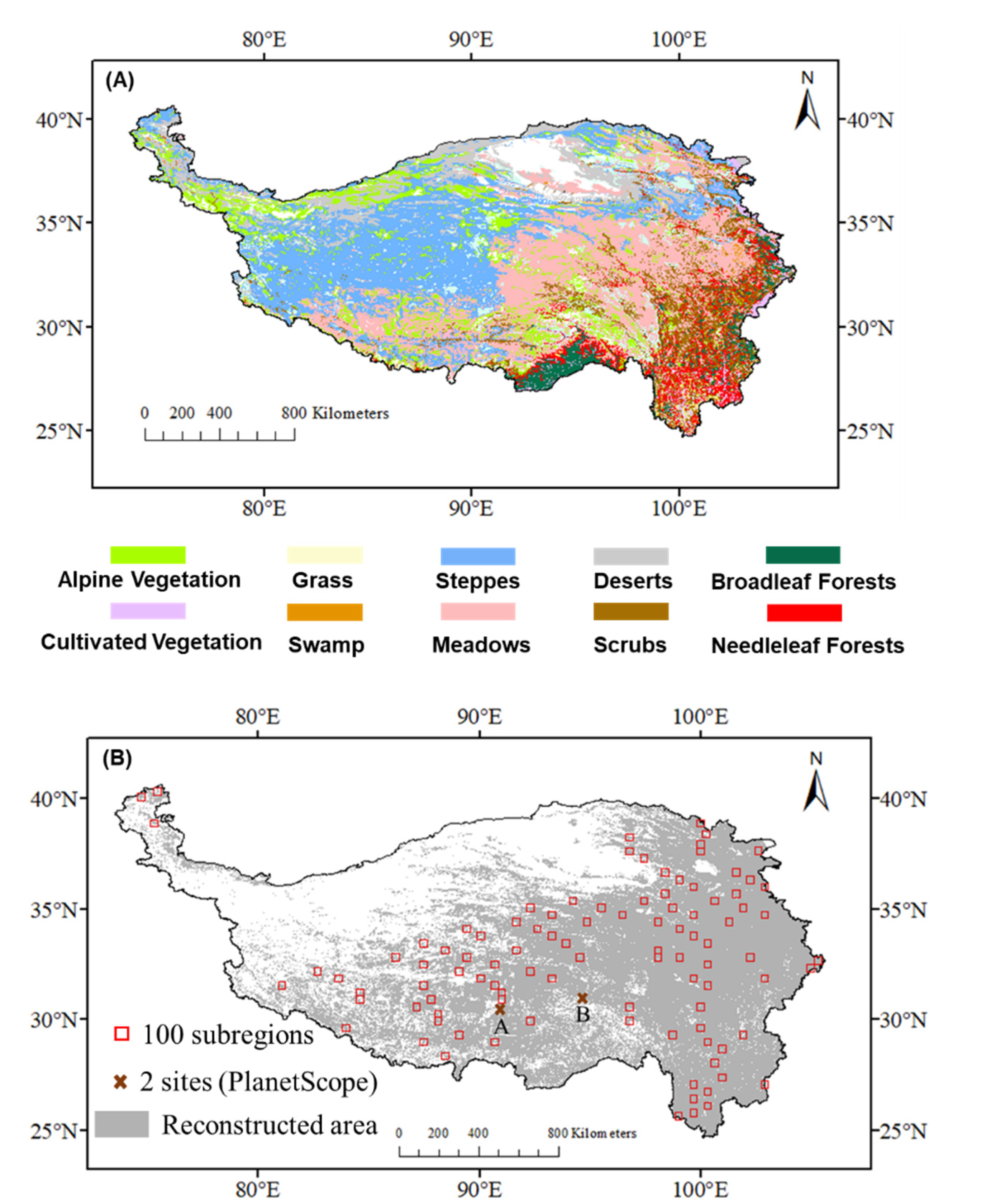
2.1. Study Area

The QTP is located in Southwest China, ranging from 25° to 40°N and from 74° to 104°E, with an area of approximately 2.5 million km2 and an average elevation above 4500 m. The main vegetation types in this alpine ecoregion include alpine steppes, meadows, scrubs, and broadleaf and needleleaf forests (see Figure 1A for the spatial distribution). We excluded nonvegetated areas from the reconstruction of Landsat NDVI time-series data. Here, nonvegetated areas on the QTP were defined as areas where the average cloud-free MODIS NDVI from July to September was lower than 0.15. The threshold of 0.15 was determined empirically. It is, indeed, true that some soil NDVI values may be larger than 0.15; however, this does not affect the practical application of the QTP-NDVI30 dataset. Users can further exclude nonvegetated areas from QTP-NDVI30 using a higher NDVI threshold. In QTP-NDVI30, the vegetated areas on the QTP are shown in Figure 1B (see the gray color).

2.2. Satellite Data

The high-spatiotemporal-resolution NDVI time-series for the QTP were reconstructed by blending the Landsat data with the MODIS data. We collected the MODIS surface-reflectance product (MOD09Q1) from the United States Geological Survey (USGS), which provides 250 m and 8-day resolution data for the red and near-infrared bands. In addition, the corresponding MODIS data-quality flags were obtained. We noticed that other MODIS NDVI products were available, such as the NDVI data estimated from the BRDF (bidirectional reflectance distribution function)-adjusted reflectance product (MCD43A4). In our previous analyses [30], we compared the fusion accuracy when using MOD09Q1 and MCD43A4 and found that better results were obtained when MOD09Q1 was performed. Notably, MOD09Q1 has a higher spatial resolution than MCD43A4 (250 m vs. 500 m), although the viewing angular differences between MODIS and Landsat data are corrected in MCD43A4. Therefore, we used MOD09Q1 in this study.
We collected all available Landsat surface-reflectance (SR) images (red and near-infrared bands) for the QTP from 2000 to 2020, except in 2012. In 2012, there were few Landsat data due to the failure of Landsat 5. Therefore, the collected Landsat data include those from the Landsat-5 TM (January 2000–December 2011), Landsat-7 ETM+ (January 2000-December 2020), and Landsat-8 OLI (February 2013–December 2020). Due to the faulty scan lines correct for Landsat-7 (referred to as SLC-off), there are missing stripes in the ETM+ images after May 2003. These SLC-off images were also included in the reconstruction process because maximizing the amount of cloud-free observation data used has been proven to be effective in enhancing the performance of MODIS–Landsat data fusion [25].

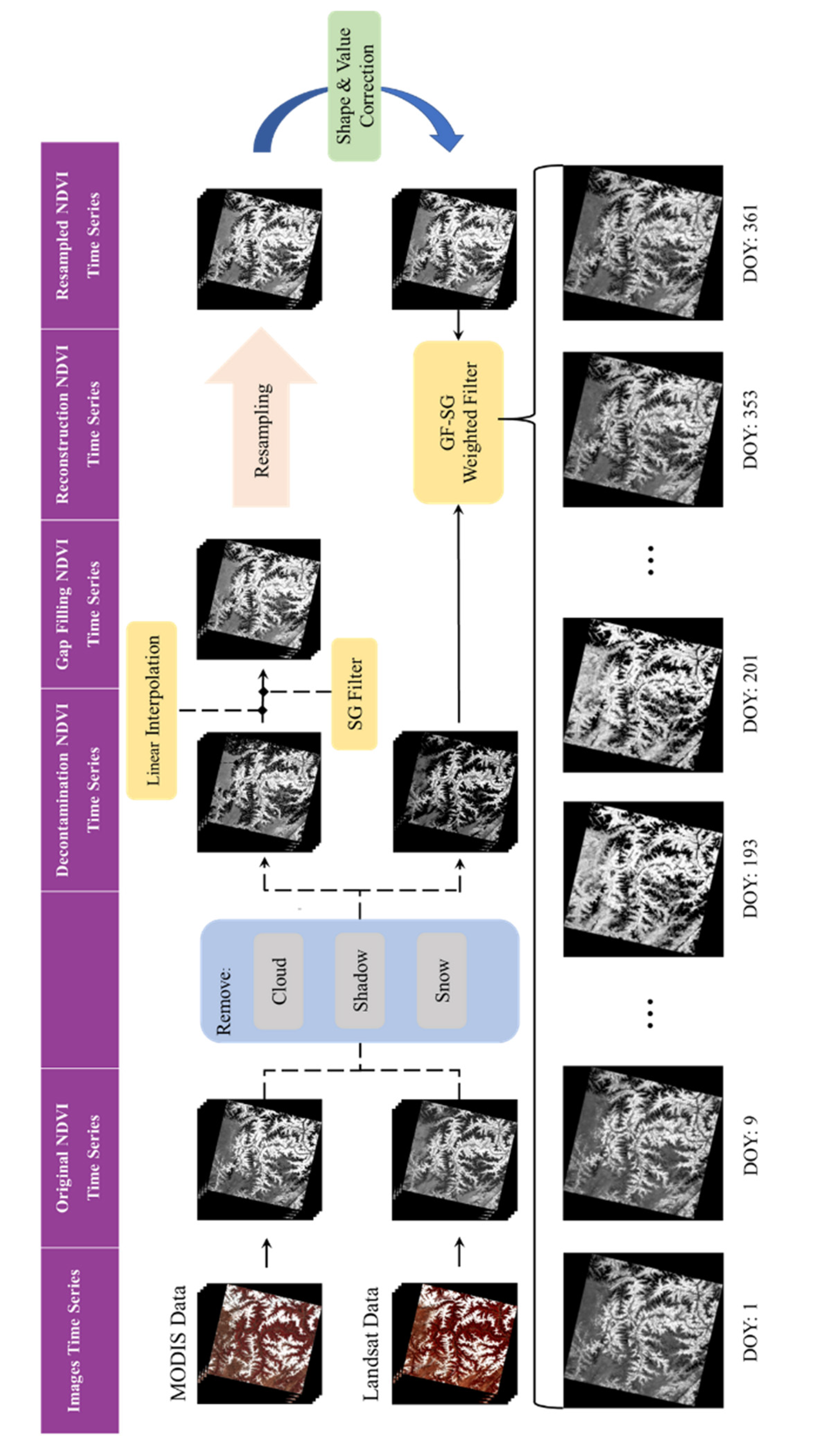
2.3. The Landsat NDVI Time-Series Data Reconstruction Method

The recently developed GF-SG method was used in the reconstruction of high-quality continuous Landsat NDVI time-series data in the QTP region (QTP-NDVI30). In general, the GF-SG method includes two main steps [30].
In the first step, GF-SG fills the missing values in the original Landsat NDVI time-series data. Because the original Landsat NDVI time-series may be relatively discontinuous and even contain few cloud-free observations within a year, it is impossible to directly fill missing values via linear interpolation or curve fitting. In the GF-SG method, MODIS NDVI images with high spatial autocorrelation are preferable, and these images can be spatially resampled to 30 m via the bicubic interpolation method (referred to as “M_interpol”). Then, GF-SG determines similar pixels of each target pixel within a local neighboring window (40 × 40 pixel, about 1.2 × 1.2 km) by calculating the correlation coefficients between M_interpol and the cloud-free Landsat observations of this target pixel. The neighboring pixels with correlation coefficients above 0.8 are assumed to be similar pixels to the target pixel ( M _ s i m i l a r _ s e r i e s ( x j , y j ) ) and can be used for generating synthesized NDVI time-series data for the target pixels; this is given by:
    M _ r e f e r e n c e ( x , y ) = j = 1 n w ( x j , y j ) × M _ s i m i l a r _ s e r i e s ( x j , y j )
where n indicates the number of similar pixels and w ( x j , y j ) represents the weight of the jth similar pixels. w ( x j , y j ) was determined according to the similarity between the time-series data of the jth similar pixels and that of the target pixel, which is quantified by the correlation coefficient between the time series of the two data. Considering the difference in the NDVI values between the Landsat and MODIS data (e.g., different spectral response function), GF-SG incorporates the concept of shape-model fitting [32,33] and uses the linear transfer function [34] to modify M _ r e f e r e n c e ( x , y ) , expressed as:
M _ a d j u s t e d ( x , y ) = M _ r e f e r e n c e ( x , y ) × a ( x , y ) + a 0 ( x , y )
where a ( x , y ) and a 0 ( x , y ) are solved by minimizing the difference between M _ a d j u s t e d ( x , y ) and the cloud-free Landsat observations of the target pixel.
In the second step of GF-SG, a weighted SG filter is used to smooth the synthesized NDVI time-series to reduce residual noise. The weighting mechanism in the GF-SG filter is based on two principles: (1) the original cloud-free Landsat observations are assumed to have the largest weights to optimally preserve these observations; and (2) in the synthesized NDVI time-series, the filled NDVI values on certain dates are assigned larger weights if the NDVI images on these dates exhibit small spatial variations, and vice versa. This principle is reasonable because spatial resampling is more reliable for homogeneous landscapes than for others. For more details regarding the GF-SG method, please refer to the study by Chen et al. [30].
Figure 2 shows the flowchart used to reconstruct continuous Landsat NDVI time-series data in the QTP region. To process the large numbers of Landsat images and data analyses required, the reconstruction was conducted in the Google Earth Engine (GEE) cloud-computing platform. Several issues in the reconstruction process should be clarified. First, to avoid excessive occupation of computing resources by individual users, the GEE platform allocates restricted computing power to individual users and does not allow the same task to be run from different user accounts. We, therefore, divided the entire QTP into four subregions to ensure that each subregion could be processed separately on the GEE. Because a local neighboring window is necessary for the generation of the synthesized NDVI time-series for each Landsat pixel, we created a 2 km buffer for each subarea to process the boundary pixels. Then, we composited the original Landsat NDVI time-series according to the MODIS imaging time (i.e., 1, 9, …, and 353, with 8-day time intervals). At each imaging time, we set the original NDVI value as the maximum value of all available Landsat 5/7/8 NDVI data within a 16-day time window (i.e., 8 days before and after each imaging time). Third, the MODIS and Landsat pixels identified as clouds, cloud shadows, and snow were removed. These missing values in the MODIS NDVI time-series were linearly interpolated. For snow contamination on the QTP, we used the first or the last snow- and cloud-free observation as a background reference to address the temporally continuous snow-contaminated values in early spring or late autumn; this step is not considered in the original GF-SG method.

2.4. Experiments and Accuracy Assessments

We evaluated QTP-NDVI30 in three experiments. In the first experiment, we selected Landsat images obtained from July to September with cloud coverages less than 50% in 100 randomly determined subregions (30 km × 30 km) distributed relatively uniformly over the QTP (see Figure 1B). One hundred random locations cover various vegetation types on the QTP, including alpine steppes, meadows, scrubs, and broadleaf and needleleaf forests (Figure 1B). Then, these selected images were removed from the reconstruction and were used as the reference data. Finally, we quantitively compared the reconstructed 30 m NDVI images with these reference Landsat images.
In the second experiment, 16 PlanetScope constellation multispectral images (3 m resolution) were collected at two test sites (Figure 1B) and were compared with QTP-NDVI30-based images. Notably, the 100 reference Landsat images were excluded from the reconstruction in the first simulation experiment, whereas all available Landsat images were included in the second experiment.
In the third experiment, we explored an application of QTP-NDVI30 to determine the vegetation green-up date (GUD) over the QTP. The GUD was estimated according to Zhang’s logistic method [35], and was determined to be the date showing an initial maximum value of the rate of change in the curvature of the fitted NDVI curve. We compared the QTP-NDVI30-derived GUD with the MODIS-derived GUD through visual assessments and expected richer spatial information in the QTP-NDVI30-derived GUD.
We used four statistical indices for quantitative assessments: the mean absolute error (MAE), relative MAE, correlation coefficient (R) and structural similarity index (SSIM). The SSIM has been widely used to assess the overall structural similarity between the reconstructed and reference images [36]. In this study, SSIM was calculated as:
SSIM = L ( r e c o n , r e f ) C ( r e c o n , r e f ) S ( r e c o n , r e f ) L ( r e c o n , r e f ) = 2 u r e c o n u r e f + c 1 u r e c o n 2 + u r e f 2 + c 1 C ( r e c o n , r e f ) = 2 σ r e c o n σ r e f + c 2 σ r e c o n 2 + σ r e f 2 + c 2 S ( r e c o n , r e f ) = σ r e c o n , r e f + c 3 σ r e c o n σ r e f + c 3
where the subscripts “recon” and “ref” represent the cloud-free pixels in the reconstructed and reference Landsat NDVI images, respectively; u r e c o n and u r e f represent the average NDVI value; σ r e c o n and σ r e f represent the NDVI standard deviation; and   σ r e c o n , r e f represents covariance.   c 1 ,   c 2 ,   c 3 are constants to avoid a zero denominator and are determined as:
C 1 = ( K 1 × L ) 2 C 2 = ( K 2 × L ) 2 C 3 = C 2 / 2
where K 1 and K 2 are equal to 0.01 and 0.03, respectively and L represents the dynamic range of pixel values for an image. The SSIM varies between 0 and 1, with larger SSIM values indicating more similar spatial patterns between the reconstructed and reference images, and vice versa.

3. Results

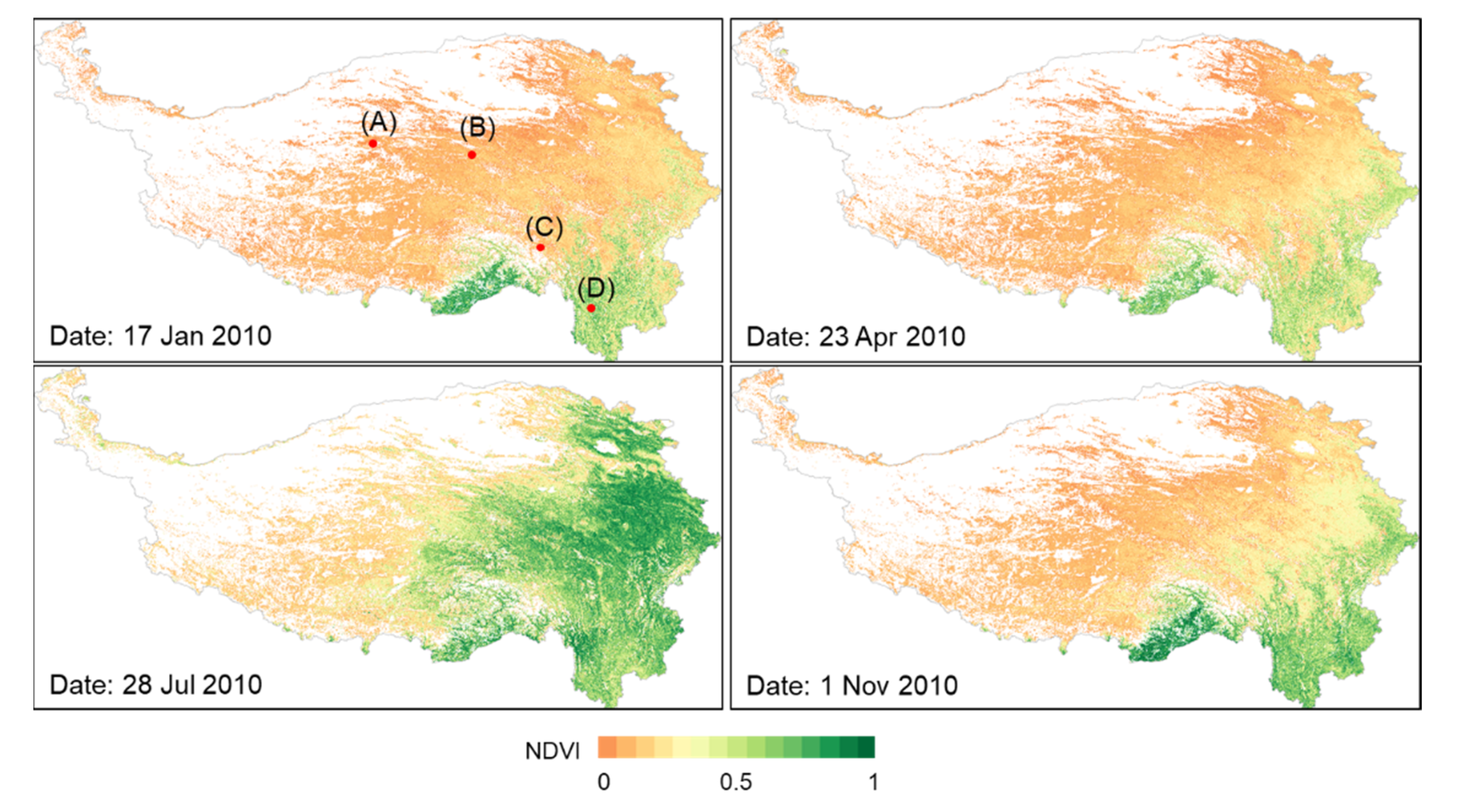
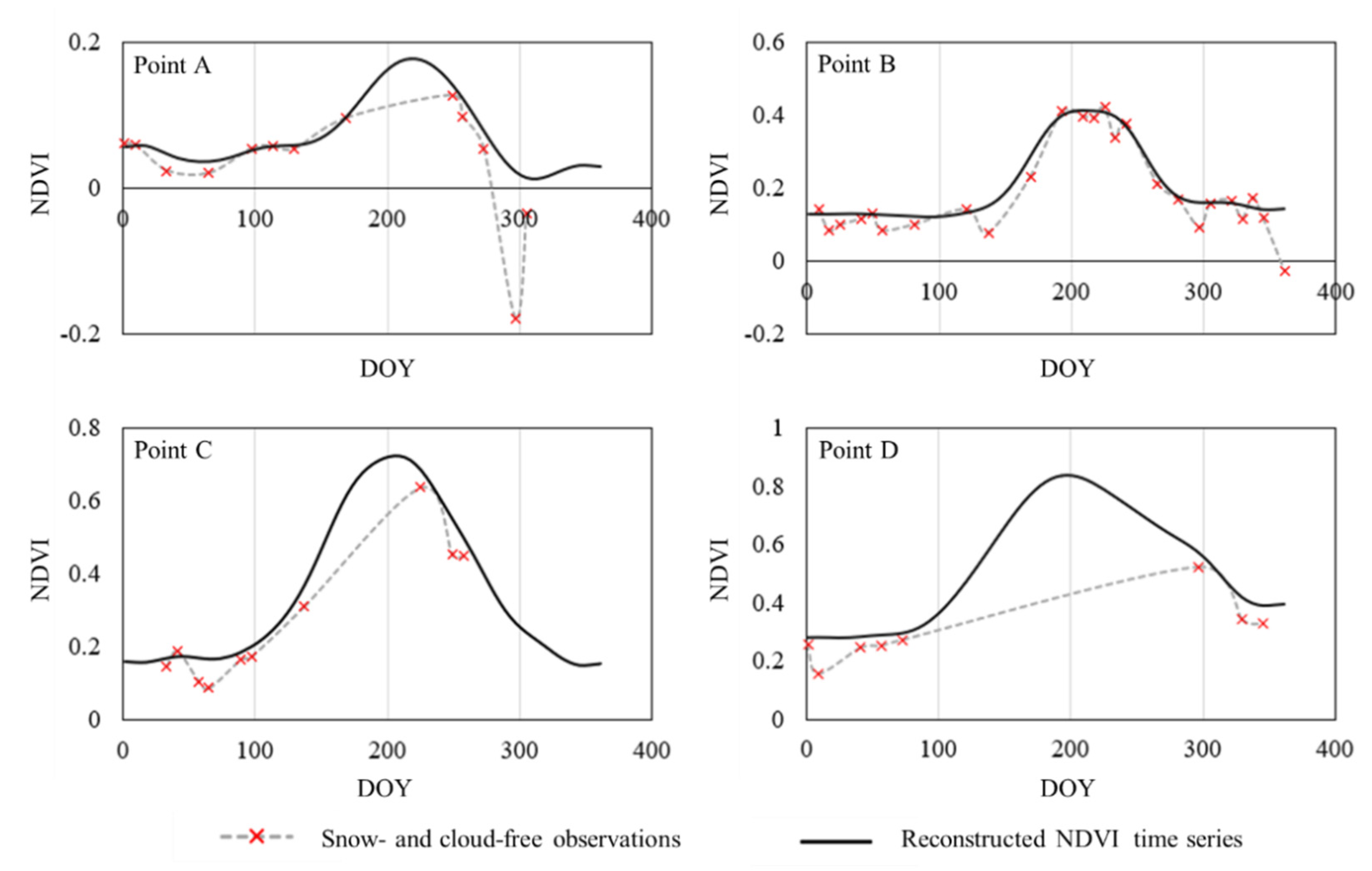
3.1. Spatiotemporal Patterns of QTP-NDVI30

Figure 3 shows the spatial distribution of the reconstructed Landsat NDVI data on four dates in 2010 (17 January, 23 April, 28 July, and 1 November). In general, the spatial variations in vegetation greenness across the QTP can be effectively captured by the reconstructed Landsat NDVI data. High NDVI values (>0.5) throughout the year are observed on the southwestern QTP, which is mainly covered by deciduous and evergreen mixed forests. In the central and northeastern QTP areas, the alpine steppe and meadow exhibit obvious seasonal greenness dynamics, with a low NDVI in winter and an increasing NDVI after grass growth in spring. Vegetation is very sparse on the northwestern QTP, with low NDVI values throughout the year. The reconstructed Landsat NDVI is spatially continuous, and the spatial pattern is consistent with our prior knowledge of the vegetation distribution in this cold and dry alpine ecoregion.
We further examined the reconstructed Landsat NDVI time-series data at four randomly selected locations (Figure 4). At location B, the cloud-free observations were relatively concentrated during the growing season (May–September). The reconstructed NDVI time-series reflect the temporal trends well, notably reaching the upper envelope of the original Landsat NDVI because of the incorporation of the iterative SG filter. The reconstructed NDVI data effectively corrected some abnormal decreases in the original NDVI time-series, such as near the start of the growing season (Point B in Figure 4). At the other three locations, the original cloud-free Landsat observations were temporally discontinuous, with some long-term gaps. Because continuous gaps may occur in the peak of the growing season, these discontinuous time-series cannot be reconstructed by using linear interpolations or temporal filters. By fusing the MODIS data, QTP-NDVI30 generates reasonable annual vegetation-growth curves. In the following experiments, we conducted quantitative assessments of QTP-NDVI30 in this challenging scenario whereby NDVI data gaps occur at the peak of the growing season.

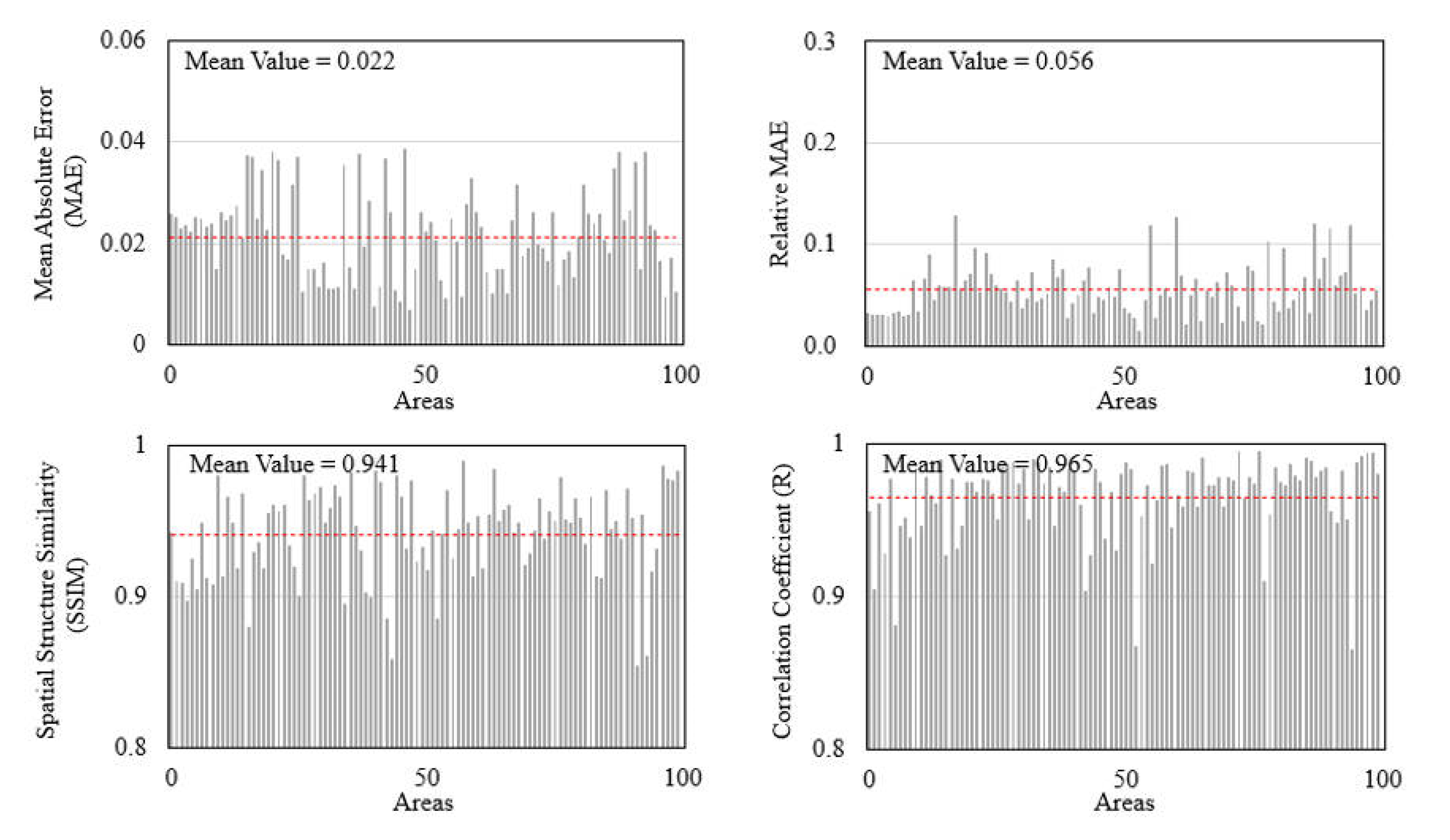
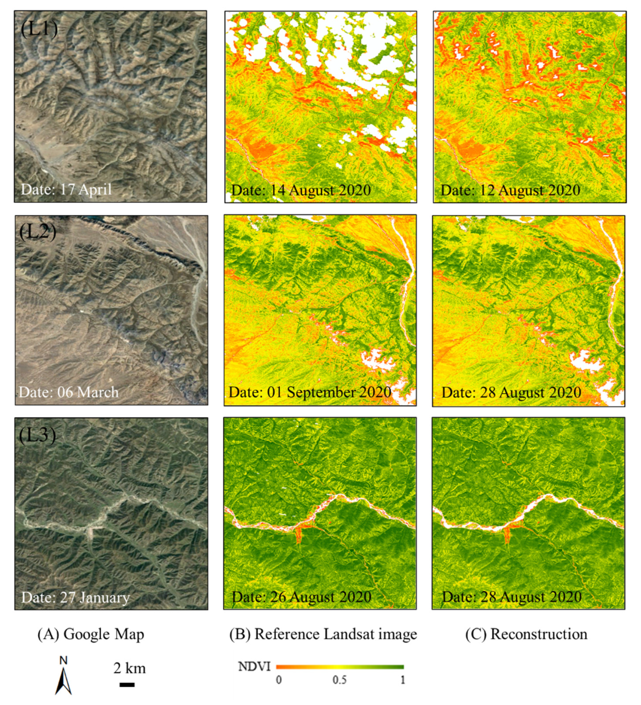
3.2. Quantitative Assessments with the Reference Landsat NDVI Images

One hundred reference Landsat images from 100 randomly selected subregions (i.e., one reference image per subregion) were excluded from the reconstruction process and used for quantitative assessments. The results show that the MAE averaged over the 100 subregions is approximately 0.02 and that the relative MAE is below 6% (Figure 5). The reconstructed Landsat NDVI images generally exhibit high spatial-structure similarity with the reference images, with average SSIM values above 0.94, indicating the satisfactory accuracy of the reconstructed Landsat NDVI time-series.
To more intuitively investigate the performance, the reconstructed Landsat NDVI images were compared with the reference images in three subregions, as shown in Figure 6. Here, it should be noted that the reference Landsat NDVI images, including those with cloud-free pixels, were not used in the reconstruction process in this experiment. The results show that the reconstructed Landsat NDVI images can effectively reflect the spatial variations in vegetation greenness in the mountain areas, and the spatial trend is consistent with that of the reference NDVI images (see Figure 6B,C). The visual comparisons suggest that the reconstructed 30 m NDVI time-series could potentially be used to estimate fine-scale vegetation parameters for land-surface process simulations.

3.3. Quantitative Assessments Using the PlanetScope NDVI Images

Recently, the PlanetScope satellite constellation was established by launching groups of individual cubes, which can provide revisit observations on a daily basis and at a very high spatial resolution. We collected 16 PlanetScope images (3 m resolution) at two test sites (Figure 1B) to compare with QTP-NDVI30-based images. There were seven and nine PlanetScope images covering sites A and B, respectively (Table 1). This experiment was conducted for two reasons. First, in the previous experiment (in Section 3.2), the 100 reference Landsat NDVI images were not used in the reconstruction process, which is somewhat limiting in terms of reflecting the actual situation. In this experiment, the reconstruction process includes all available Landsat data. Second, the PlanetScope constellation data are commercial satellite data that are too expensive and cannot meet the requirement of long-term monitoring on the QTP. However, the PlanetScope constellation data can provide higher-spatiotemporal-resolution images. In this experiment, we aim to further investigate the difference between the PlanetScope NDVI images and the reconstructed Landsat NDVI images.
The consistency between the two NDVI datasets was quantitatively evaluated using the correlation coefficient (R) and SSIM (Table 1). To calculate the R and SSIM values, the 3 m PlanetScope data were resampled to 30 m using an aggregation method. Given the difference between the PlanetScope and Landsat sensors (in terms of the spectral-response function and point-spread function), we did not calculate the MAE values between the two datasets. The results show that the R values are between 0.78 and 0.87, with an average value of 0.83, and the SSIM values range from 0.77 to 0.95, with an average SSIM of 0.87 (Table 1), reflecting acceptable accuracy considering the comparisons were made using data from two different sensors.
We further compared the spatial patterns among the PlanetScope NDVI (3 m), MODIS NDVI (250 m), original Landsat NDVI (30 m), and QTP-NDVI30 (30 m) in the A-5 and B-8 areas (Figure 7 and Figure 8). We found that the 250 m MODIS NDVI data do not reflect fine-scale greenness variations. For example, in the B-8 area (Figure 8), the alpine terrain highly influences the spatial pattern of NDVI (see the enlarged view of the PlanetScope data), and this effect cannot be simulated using the MODIS NDVI. The cloud-contaminated pixels in the original Landsat NDVI images are successfully reconstructed in the QTP-NDVI30 imagery. For example, green vegetation distributed in some very small local areas of A-5 can be captured by QTP-NDVI30 (Figure 7E). Improving the spatial resolution from 250 m to 30 m with QTP-NDVI30 obviously enhances the spatial details of the NDVI in heterogeneous topographic regions. Additionally, marginal improvements in the spatial details of the NDIV are achieved with the transformation from a resolution of 30 m to 3 m (Figure 7 and Figure 8).

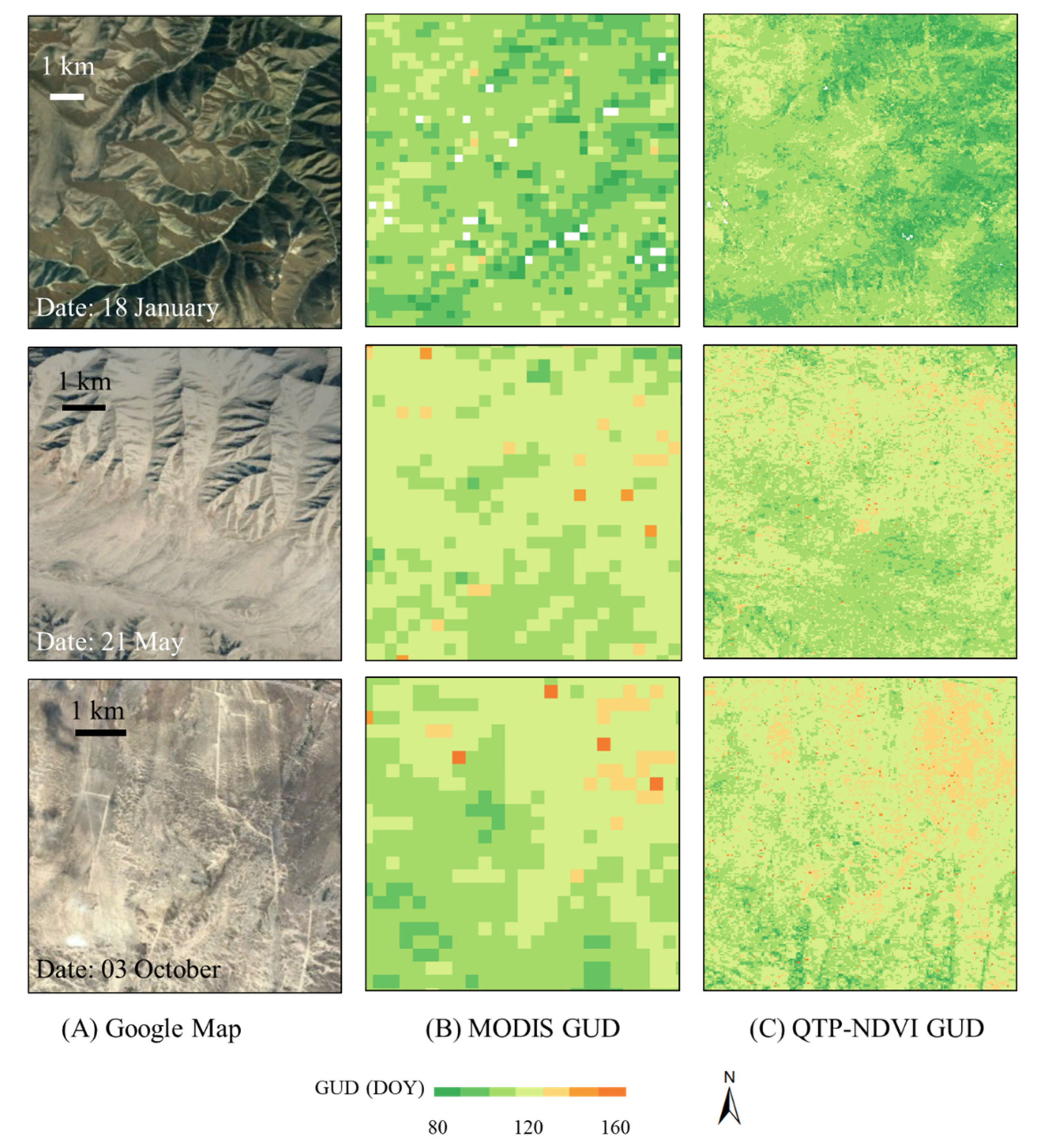
3.4. An Application of QTP-NDVI30 to Detect Vegetation Phenology

As a key phenological-stage indicator, the green-up date (GUD) characterizes the start of vegetation growth and can be estimated from NDVI time-series. Previous studies have normally used MODIS NDVI data to estimate the GUD on the QTP [5,37]. The generated QTP-NDVI30 product provides an opportunity to determine the GUD at a 30 m spatial scale. In this experiment, we estimated the GUD using the widely used logistic fitting method [35], and the GUD was defined as the date on which the rate of change in the curvature of the fitted NDVI curve reached an initial maximum. The pixels without obvious seasonal NDVI changes were excluded from the estimates [5]. We compared the GUD estimates derived from the MODIS and QTP-NDVI30 data in 2018. The results show that the QTP-NDVI30-derived GUD exhibits a spatial pattern similar to that of the MODIS-derived GUD over the entire QTP, with earlier GUDs in the northeastern QTP area and later GUDs in the southwestern part of the plateau (Figure 9). However, QTP-NDVI30-derived GUDs better describe detailed spatial variations in the actual GUD at the derived 30 m spatial resolution (Figure 10). For example, 250 m MODIS GUD data exhibit obvious block effects in enlarged local areas (Figure 10B). In contrast, QTP-NDVI30-derived GUD maps capture subpixel GUD variations with rich spatial details.

4. Discussion

4.1. The Value and Robustness of the QTP-NDVI30 Data

The QTP-NDVI30 data were reconstructed based mainly on our recently developed GF-SG method. The GF-SG method effectively incorporates three types of auxiliary information: spatial similarity, spatial autocorrelation, and temporal-change information. In previous tests at two heterogeneous cropland sites [30], the GF-SG method outperformed three other typical Landsat NDVI reconstruction methods (IFSDAF, Liu et al. [38]; STAIR, Luo et al. [39]; and Fill-and-Fit, Yan et al. [24]). Two improvements make the GF-SG method particularly suitable for the reconstruction of Landsat NDVI time-series on the QTP. First, on the QTP, continuous Landsat NDVI gaps are very common during the growing season due to frequent cloud contamination in summer (Figure 4). This challenging issue can be effectively resolved using the GF-SG method, which has been proven to be reliable in reconstructing continuous long-term NDVI gaps (see Figure 9 of Chen et al. [30]). Second, Landsat cloud-detection errors can be serious in the QTP region, which can further decrease the ease of cloud removal (see Figure 5 of Cao et al. [28]). The GF-SG method includes a weighted Savitzky–Golay filter that corrects residual noise in NDVI time-series; thus, the performance of this method is less affected by cloud-detection errors. These strengths of the GF-SG method ensure the robustness of the QTP-NDVI30 data, as confirmed by our experiments in terms of both quantitative assessments (the average SSIM value is greater than 0.94; Figure 5) and visual inspections (Figure 6 and Figure 8).
QTP-NDVI30 provides continuous NDVI data with a 30 m spatial resolution, thus improving our ability to monitor vegetation dynamics in variable topographic areas and providing a potential resource for the research community. Our experiments show the superiority of QTP-NDVI30 in simulating fine-scale vegetation phenology (Figure 10). The coupling influence between climate factors and terrain effects on vegetation phenology can, therefore, be investigated using QTP-NDVI30. In addition, fine-scale vegetation coverage parameters in each 15-day period are among the factors used as inputs in soil-erosion simulations in the QTP region using the Chinese Soil Loss Equation (CSLE) [22]. These high-spatiotemporal-resolution vegetation parameters can be estimated from QTP-NDVI30. Reconstructions of continuous Landsat NDVI time-series for the QTP can be enhanced through progress in reconstruction algorithms and cloud computing. However, it still takes nearly half a year to generate QTP-NDVI30 data with the GEE platform for two main reasons. First, all available Landsat images from 2000–2020 in the QTP area are employed, which requires large quantities of computations and many data analysis processes. Second, the GEE platform restricts the computing power of individual users. Google accounts may be forbidden if they are used to run the same task repeatedly on the GEE. Therefore, it is necessary to release QTP-NDVI30 after careful data assessments to fully support ecological research on the QTP, particularly in the context of climate warming.

4.2. Limitations of QTP-NDVI30

Several limitations remain for QTP-NDVI30. First, QTP-NDVI30 currently only spans 2000 to 2020 because the MODIS observations date back to 2000. Before the era of MODIS, AVHRR NDVI time-series (1982–1999) were the unique auxiliary data source for spatiotemporal NDVI fusion. However, there may be much higher uncertainty in AVHRR–Landsat data fusion due to the large difference in spatial resolution between the two datasets (4–8 km vs. 30 m) and low data quality of the AVHRR NDVI [5]. For these reasons, 30 m NDVI data before 2000 were not reconstructed. Second, the SLC-off Landsat 7 data after May 2003 were included in the generation of QTP-NDVI30. It is possible that pixels inside and outside the missing stripes were reconstructed using different numbers of images, resulting in less-spatially-smooth reconstructed NDVI images in some local areas. Notably, we performed QTP-NDVI30 reconstruction without using SLC-off Landsat 7 data, but observed obvious increases in the MAE (data not shown). Third, a small number of vegetation pixels in the QTP region (< 1%) failed to be reconstructed in QTP-NDVI30. The reason for this issue is poor quality (e.g., continuous missing values) in the MODIS time-series data of these pixels. As a result, the reference shape within the local window was not found for these pixels when using the GF-SG method. Two solutions may be considered to address this issue. One is to define a lower threshold (the original value is 0.8 in the GF-SG method) to search for the reference shape if a certain degree of accuracy variation is allowed. The other is to employ climate variables (e.g., temperature and precipitation) to simulate vegetation growth trajectories for these pixels [40,41]. In QTP-NDVI30, the two solutions were not used to further process the unreconstructed vegetation pixels by considering the small percentage of these pixels, which will not affect the practical application of QTP-NDVI30.

5. Conclusions

Currently, MODIS provides the highest-spatial-resolution (250 m) NDVI time-series data for ecological research on the QTP. However, vegetation monitoring in topographic regions requires NDVI time-series data with a higher spatial resolution. To fill this gap, in this study, we reconstructed an 8-day and 30 m resolution NDVI dataset for the QTP from 2000–2020. The obtained NDVI dataset (referred to as QTP-NDVI30) was produced by employing all available Landsat 5/7/8 images (>100,000 scenes) with the developed spatiotemporal GF-SG data-fusion algorithm. QTP-NDVI30 was carefully evaluated, and the subsequent results displayed satisfactory accuracy. Compared with the reference Landsat images in 100 randomly selected subregions across the QTP, the reconstructed NDVI data achieved an average MAE of 0.02 and average SSIM values greater than 0.94. QTP-NDVI30 displays similar spatial variations in vegetation greenness to the PlanetScope images, whereas the rich spatial details cannot be simulated by the 250 m MODIS NDVI product. QTP-NDVI30 has excellent potential for use in vegetation monitoring and land-surface process models related to fine-scale vegetation parameters. In the future, we will update QTP-NDVI30 by generating the data from after 2020. In the QTP-NDVI30 dataset, one image file corresponds to an NDVI image for the entire QTP on one date (~13 gigabytes). QTP-NDVI30 will be uploaded to the National Tibetan Plateau Data Center (TPDC) and is freely available for scientific research. To acquire the download link, please contact the corresponding author.

Author Contributions

Conceptualization, R.C.; methodology, R.C. and Z.X.; validation, Z.X.; writing—original draft preparation, R.C.; writing—review and editing, Y.C., J.C. and M.S.; funding acquisition, R.C. All authors have read and agreed to the published version of the manuscript.

Funding

This work was funded by the second Scientific Expedition to the Qinghai-Tibet Plateau (2019QZKK0307) and the Sichuan Science and Technology Program (2021YFG0028 and 2022YFH0106).

Data Availability Statement

All Landsat data used in this study can be obtained from the USGS EarthExplorer website (https://earthexplorer.usgs.gov/). QTP-NDVI30 will be uploaded to the National Tibetan Plateau Data Center (TPDC) and is freely available for scientific research. To acquire the download link, please contact the corresponding author.

Conflicts of Interest

The authors declare no conflict of interest.

References

  1. You, Q.; Min, J.; Kang, S. Rapid warming in the Tibetan Plateau from observations and CMIP5 models in recent decades. Int. J. Climatol. 2016, 36, 2660–2670. [Google Scholar] [CrossRef]
  2. Li, P.; Zhu, D.; Wang, Y.; Liu, D. Elevation dependence of drought legacy effects on vegetation greenness over the Tibetan Plateau. Agric. For. Meteorol. 2020, 295, 108190. [Google Scholar] [CrossRef]
  3. Zhang, L.; Guo, H.; Wang, C.; Ji, L.; Li, J.; Wang, K.; Dai, L. The long-term trends (1982–2006) in vegetation greenness of the alpine ecosystem in the Qinghai-Tibetan Plateau. Environ. Earth Sci. 2014, 72, 1827–1841. [Google Scholar] [CrossRef]
  4. Liang, S.; Lv, C.; Wang, G.; Feng, Y.; Wu, Q.; Wan, L.; Tong, Y. Vegetation phenology and its variations in the Tibetan Plateau, China. Int. J. Remote Sens. 2019, 40, 3323–3343. [Google Scholar] [CrossRef]
  5. Shen, M.; Zhang, G.; Cong, N.; Wang, S.; Kong, W.; Piao, S. Increasing altitudinal gradient of spring vegetation phenology during the last decade on the Qinghai–Tibetan Plateau. Agric. For. Meteorol. 2014, 189, 71–80. [Google Scholar] [CrossRef]
  6. Zhang, Q.; Kong, D.; Shi, P.; Singh, V.P.; Sun, P. Vegetation phenology on the Qinghai-Tibetan Plateau and its response to climate change (1982–2013). Agric. For. Meteorol. 2018, 248, 408–417. [Google Scholar] [CrossRef]
  7. Dong, S.; Shang, Z.; Gao, J.; Boone, R.B. Enhancing sustainability of grassland ecosystems through ecological restoration and grazing management in an era of climate change on Qinghai-Tibetan Plateau. Agric. Ecosyst. Environ. 2020, 287, 106684. [Google Scholar] [CrossRef]
  8. Körner, C.; Jetz, W.; Paulsen, J.; Payne, D.; Rudmann-Maurer, K.; Spehn, E.M. A global inventory of mountains for bio-geographical applications. Alp. Bot. 2017, 127, 1–15. [Google Scholar] [CrossRef] [Green Version]
  9. Tucker, C.J. Red and photographic infrared linear combinations for monitoring vegetation. Remote Sens. Environ. 1979, 8, 127–150. [Google Scholar] [CrossRef] [Green Version]
  10. Atzberger, C.; Eilers, P.H. A time series for monitoring vegetation activity and phenology at 10-daily time steps covering large parts of South America. Int. J. Digit. Earth 2011, 4, 365–386. [Google Scholar] [CrossRef]
  11. Cao, R.; Chen, Y.; Shen, M.; Chen, J.; Zhou, J.; Wang, C.; Yang, W. A simple method to improve the quality of NDVI time-series data by integrating spatiotemporal information with the Savitzky-Golay filter. Remote Sens. Environ. 2018, 217, 244–257. [Google Scholar] [CrossRef]
  12. Chen, J.; Jönsson, P.; Tamura, M.; Gu, Z.; Matsushita, B.; Eklundh, L. A simple method for reconstructing a high-quality NDVI time-series data set based on the Savitzky–Golay filter. Remote Sens. Environ. 2004, 91, 332–344. [Google Scholar] [CrossRef]
  13. Zhu, W.; Pan, Y.; He, H.; Wang, L.; Mou, M.; Liu, J. A changing-weight filter method for reconstructing a high-quality NDVI time series to preserve the integrity of vegetation phenology. IEEE Trans. Geosci. Remote Sens. 2011, 50, 1085–1094. [Google Scholar] [CrossRef]
  14. Cao, R.; Chen, Y.; Chen, J.; Zhu, X.; Shen, M. Thick cloud removal in Landsat images based on autoregression of Landsat time-series data. Remote Sens. Environ. 2020, 249, 112001. [Google Scholar] [CrossRef]
  15. Ju, J.; Roy, D.P. The availability of cloud-free Landsat ETM+ data over the conterminous United States and globally. Remote Sens. Environ. 2008, 112, 1196–1211. [Google Scholar] [CrossRef]
  16. Shen, H.; Li, X.; Cheng, Q.; Zeng, C.; Yang, G.; Li, H.; Zhang, L. Missing information reconstruction of remote sensing data: A technical review. IEEE Geosci. Remote Sens. Mag. 2015, 3, 61–85. [Google Scholar] [CrossRef]
  17. An, S.; Zhang, X.; Chen, X.; Yan, D.; Henebry, G.M. An exploration of terrain effects on land surface phenology across the Qinghai–Tibet plateau using Landsat ETM+ and OLI data. Remote Sens. 2018, 10, 1069. [Google Scholar] [CrossRef] [Green Version]
  18. Chen, F.; Liu, Z.; Zhong, H.; Wang, S. Exploring the Applicability and Scaling Effects of Satellite-Observed Spring and Autumn Phenology in Complex Terrain Regions Using Four Different Spatial Resolution Products. Remote Sens. 2021, 13, 4582. [Google Scholar] [CrossRef]
  19. An, S.; Zhu, X.; Shen, M.; Wang, Y.; Cao, R.; Chen, X.; Yang, W.; Chen, J.; Tang, Y. Mismatch in elevational shifts between satellite observed vegetation greenness and temperature isolines during 2000–2016 on the Tibetan Plateau. Glob. Chang. Biol. 2018, 24, 5411–5425. [Google Scholar] [CrossRef]
  20. Lu, L.; Shen, X.; Cao, R. Elevational Movement of Vegetation Greenness on the Tibetan Plateau: Evidence from the Landsat Satellite Observations during the Last Three Decades. Atmosphere 2021, 12, 161. [Google Scholar] [CrossRef]
  21. Pan, Y.; Wang, Y.; Zheng, S.; Huete, A.R.; Shen, M.; Zhang, X.; Huang, J.; He, G.; Yu, L.; Xu, X. Characteristics of Greening along Altitudinal Gradients on the Qinghai–Tibet Plateau Based on Time-Series Landsat Images. Remote Sens. 2022, 14, 2408. [Google Scholar] [CrossRef]
  22. Duan, X.; Bai, Z.; Rong, L.; Li, Y.; Ding, J.; Tao, Y.; Li, J.; Li, J.; Wang, W. Investigation method for regional soil erosion based on the Chinese Soil Loss Equation and high-resolution spatial data: Case study on the mountainous Yunnan Province, China. Catena 2020, 184, 104237. [Google Scholar] [CrossRef]
  23. Wilson, B.T.; Knight, J.F.; McRoberts, R.E. Harmonic regression of Landsat time series for modeling attributes from national forest inventory data. ISPRS J. Photogramm. Remote Sens. 2018, 137, 29–46. [Google Scholar] [CrossRef]
  24. Yan, L.; Roy, D.P. Spatially and temporally complete Landsat reflectance time series modelling: The fill-and-fit approach. Remote Sens. Environ. 2020, 241, 111718. [Google Scholar] [CrossRef]
  25. Chen, Y.; Cao, R.; Chen, J.; Zhu, X.; Zhou, J.; Wang, G.; Shen, M.; Chen, X.; Yang, W. A new cross-fusion method to automatically determine the optimal input image pairs for NDVI spatiotemporal data fusion. IEEE Trans. Geosci. Remote Sens. 2020, 58, 5179–5194. [Google Scholar] [CrossRef]
  26. Rao, Y.; Zhu, X.; Chen, J.; Wang, J. An improved method for producing high spatial-resolution NDVI time series datasets with multi-temporal MODIS NDVI data and Landsat TM/ETM+ images. Remote Sens. 2015, 7, 7865–7891. [Google Scholar] [CrossRef] [Green Version]
  27. Zhu, X.; Helmer, E.H.; Gao, F.; Liu, D.; Chen, J.; Lefsky, M.A. A flexible spatiotemporal method for fusing satellite images with different resolutions. Remote Sens. Environ. 2016, 172, 165–177. [Google Scholar] [CrossRef]
  28. Cao, R.; Feng, Y.; Chen, J.; Zhou, J. A Supplementary Module to Improve Accuracy of the Quality Assessment Band in Landsat Cloud Images. Remote Sens. 2021, 13, 4947. [Google Scholar] [CrossRef]
  29. Zhang, Q.; Yuan, Q.; Li, J.; Li, Z.; Shen, H.; Zhang, L. Thick cloud and cloud shadow removal in multitemporal imagery using progressively spatio-temporal patch group deep learning. ISPRS J. Photogramm. Remote Sens. 2020, 162, 148–160. [Google Scholar] [CrossRef]
  30. Chen, Y.; Cao, R.; Chen, J.; Liu, L.; Matsushita, B. A practical approach to reconstruct high-quality Landsat NDVI time-series data by gap filling and the Savitzky–Golay filter. ISPRS J. Photogramm. Remote Sens. 2021, 180, 174–190. [Google Scholar] [CrossRef]
  31. Zhang, X.; Sun, S.; Yong, S.; Zhou, Z.; Wang, R. Vegetation Map of the People’s Republic of China (1:1,000,000); Geology Publishing House: Beijing, China, 2007. [Google Scholar]
  32. Liu, L.; Cao, R.; Chen, J.; Shen, M.; Wang, S.; Zhou, J.; He, B. Detecting crop phenology from vegetation index time-series data by improved shape model fitting in each phenological stage. Remote Sens. Environ. 2022, 277, 113060. [Google Scholar] [CrossRef]
  33. Sakamoto, T.; Wardlow, B.D.; Gitelson, A.A.; Verma, S.B.; Suyker, A.E.; Arkebauer, T.J. A two-step filtering approach for detecting maize and soybean phenology with time-series MODIS data. Remote Sens. Environ. 2010, 114, 2146–2159. [Google Scholar] [CrossRef]
  34. Steven, M.D.; Malthus, T.J.; Baret, F.; Xu, H.; Chopping, M.J. Intercalibration of vegetation indices from different sensor systems. Remote Sens. Environ. 2003, 88, 412–422. [Google Scholar] [CrossRef]
  35. Zhang, X.; Friedl, M.A.; Schaaf, C.B.; Strahler, A.H.; Hodges, J.C.; Gao, F.; Reed, B.C.; Huete, A. Monitoring vegetation phenology using MODIS. Remote Sens. Environ. 2003, 84, 471–475. [Google Scholar] [CrossRef]
  36. Wang, Z.; Bovik, A.C.; Sheikh, H.R.; Simoncelli, E.P. Image quality assessment: From error visibility to structural similarity. IEEE Trans. Image Process. 2004, 13, 600–612. [Google Scholar] [CrossRef] [Green Version]
  37. Cao, R.; Shen, M.; Zhou, J.; Chen, J. Modeling vegetation green-up dates across the Tibetan Plateau by including both seasonal and daily temperature and precipitation. Agric. For. Meteorol. 2018, 249, 176–186. [Google Scholar] [CrossRef]
  38. Liu, M.; Yang, W.; Zhu, X.; Chen, J.; Chen, X.; Yang, L.; Helmer, E.H. An Improved Flexible Spatiotemporal DAta Fusion (IFSDAF) method for producing high spatiotemporal resolution normalized difference vegetation index time series. Remote Sens. Environ. 2019, 227, 74–89. [Google Scholar] [CrossRef]
  39. Luo, Y.; Guan, K.; Peng, J. STAIR: A generic and fully-automated method to fuse multiple sources of optical satellite data to generate a high-resolution, daily and cloud-/gap-free surface reflectance product. Remote Sens. Environ. 2018, 214, 87–99. [Google Scholar] [CrossRef]
  40. Qiu, T.; Song, C.; Clark, J.S.; Seyednasrollah, B.; Rathnayaka, N.; Li, J. Understanding the continuous phenological development at daily time step with a bayesian hierarchical space-time model: Impacts of climate change and extreme weather events. Remote Sens. Environ. 2020, 247, 111956. [Google Scholar] [CrossRef]
  41. Seyednasrollah, B.; Swenson, J.J.; Domec, J.-C.; Clark, J.S. Leaf phenology paradox: Why warming matters most where it is already warm. Remote Sens. Environ. 2018, 209, 446–455. [Google Scholar] [CrossRef]
Figure 1. (A) The spatial distribution of the main vegetation types on the QTP, provided by The Vegetation Map of the Editorial Board of China (CAS) [31]; (B) the vegetated areas in the QTP (gray color), where NDVI reconstruction was performed. The red squares represent the 100 randomly selected subregions for quantitative assessment with reference Landsat images. The two red crosses indicate the sites for which corresponding images were compared with PlanetScope images.
Remotesensing 14 03648 g001
Figure 2. Flowchart used to reconstruct continuous Landsat NDVI time-series data for the QTP region.
Remotesensing 14 03648 g002
Figure 3. The spatial distribution of the reconstructed Landsat NDVI data in the year 2010 on four dates in different seasons. In the first panel, the NDVI time-series data of the four points A–D are shown in Figure 4.
Remotesensing 14 03648 g003
Figure 4. The original snow- and cloud-free Landsat observations (red cross) and the reconstructed Landsat NDVI time-series data at four locations (the locations are shown in Figure 3A).
Remotesensing 14 03648 g004
Figure 5. The quantitative assessments in 100 randomly selected subregions. One original Landsat image from July to September in each subregion was excluded from the reconstruction process and used as a reference image. The red dashed lines in each panel represent the values averaged over the 100 subregions.
Remotesensing 14 03648 g005
Figure 6. Comparisons between the reference Landsat NDVI images (B) and the reconstructed Landsat NDVI images (C) in the three subregions. The landscapes of the three subregions from Google Maps are shown (A). Note: the reference Landsat NDVI images, including those with cloud-free pixels, were not used in the reconstruction process.
Remotesensing 14 03648 g006
Figure 7. Comparisons of the spatial patterns of the PlanetScope NDVI (3 m), MODIS NDVI (250 m), original Landsat NDVI (30 m), and QTP-NDVI30 (30 m) in the A-5 area.
Remotesensing 14 03648 g007
Figure 8. The same as Figure 7 but for the B-8 area.
Remotesensing 14 03648 g008
Figure 9. The green-up date (GUD) estimated from 250 m MODIS NDVI time-series (upper) and QTP-NDVI30 data (lower) in 2018 for the QTP. The three local areas (points a–c) are enlarged and shown in Figure 10. Note: pixels without obvious seasonal NDVI changes were excluded from GUD estimates.
Remotesensing 14 03648 g009
Figure 10. Comparisons between the MODIS-derived 250 m GUD and the QTP-NDVI30-derived GUD in three local areas (points a–c in Figure 9). The high-resolution Google Earth images (left) are included to show landscapes. Google Earth images could not be obtained for the growing season due to availability limitations.
Remotesensing 14 03648 g010
Table 1. Comparisons between the PlanetScope images (resampled to 30 m) and QTP-NDVI30-based images at two test sites. Seven and nine PlanetScope images were available for sites A and B (Figure 1B), respectively.
Area IDDateCorrelation Coefficient (R)SSIM
A-121 June 20190.85680.9037
A-221 June 20190.83840.9299
A-321 June 20190.86920.8994
A-421 June 20190.83220.9028
A-521 June 20190.83040.8422
A-621 June 20190.78960.9501
A-721 June 20190.86120.9245
B-15 August 20100.80210.9046
B-25 August 20100.78790.8347
B-35 August 20100.80990.9069
B-45 August 20100.81140.7879
B-55 August 20100.80430.7758
B-65 August 20100.79130.7958
B-75 August 20100.83220.8358
B-85 August 20100.83080.8564
B-95 August 20100.85760.9350
Average 0.82530.8741
Publisher’s Note: MDPI stays neutral with regard to jurisdictional claims in published maps and institutional affiliations.

