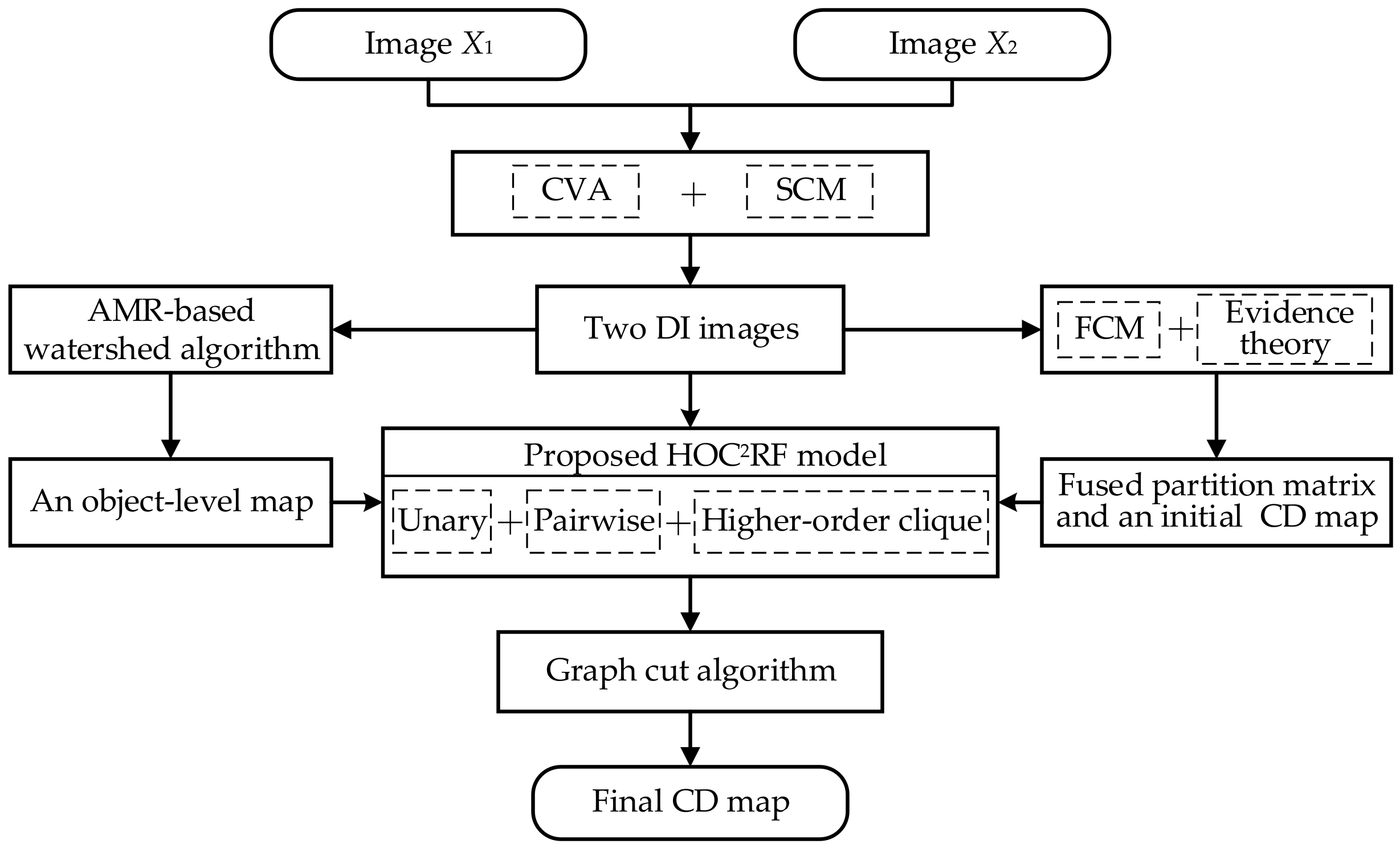
In HOC
2RF,
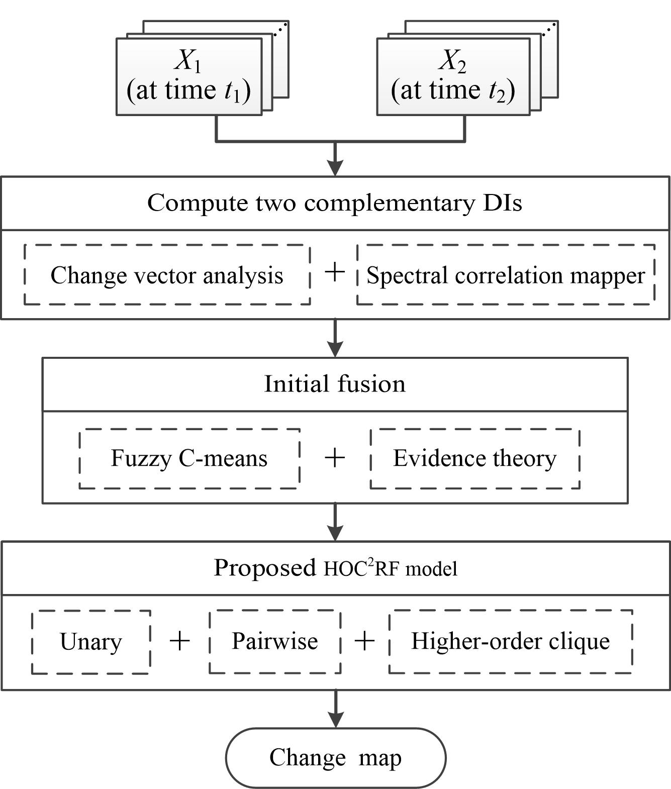
X is defined based on the two complementary DIs,
DICVA and
DISCM (obtained in
Section 3.2). In particular,
X =
DI = {
DICVA,
DISCM,
DImean},
DImean = (
DICVA +
DISCM)/2, and
xi = {
DICVA(
i),
DISCM(
i),
DImean(
i)}. The initial class label
yi for the labeling field is obtained by combining
DICVA and
DISCM (see
Section 3.3). Then, the energy function of the proposed HOC
2RF is defined as follows:
where
and
represent the unary, the pairwise, and the proposed higher-order clique potentials, respectively.
Ni denotes the neighborhood of pixel
I, and
j ∈
Ni denotes the neighboring pixel of pixel
i. In this study, the widely used second-order (i.e., the eight neighbors) neighborhood system is used to define
Ni.
S is the set composed of the image objects from the object-level map produced in
Section 3.4,
o represents an image object,
vo represents the higher-order clique of objects for
o (see Equation (15)), and the parameter
λ is the weight coefficient used to control the weight of the pairwise potential.
3.5.1. Unary and Pairwise Potentials
The unary potential function
is used to describe the relationship between the labeling and observation fields.
denotes the cost of pixel
i taking the class label
yi given the observed data and is usually defined as the negative logarithm of the probability of pixel
i belonging to class
yi:
where
P(
yi) represents the probability of pixel
i to class
yi,
yi ∈{
Cu,
Cc}, and log is the natural logarithm operator.
P(
yi) can be computed with different techniques, such as FCM. In this study,
P(
yi) is defined using the joint mass function that is obtained by combining the two complementary DIs
DICVA and
DISCM with FCM and evidence theory (see
Section 3.2 and
Section 3.3). This is
where
mi(
Cu) and
mi(
Cc) represent the combined mass values of pixel
i to the no-change and change classes, respectively (see
Section 3.3).
The pairwise potential function
is used to utilize the spatial correlation of an image in local neighborhood, and to model the interaction between pixel
i and its neighboring pixels
j in
Ni. It imposes a label constraint on the image by constraining the class labels to be consistent, by which the adjacent pixels with similar spectral values are encouraged to take the same class label. Following [
15], the pairwise potential term in (11) is written as follows:
where
d(
xi,
xj) is the Euclidean distance of
xi and
xj, respectively:
xi = {
DICVA(
i),
DISCM(
i),
DImean(
i)} and
xj = {
DICVA(
j),
DISCM(
j),
DImean(
j)}.
is the mean value of
d(
xi,
xj) over the neighborhood
Ni.
3.5.2. Proposed Higher-Order Clique Potential
The higher-order potential (object term) was introduced into the CD task in [
21] to enhance CD performance. However, the higher-order potential in [
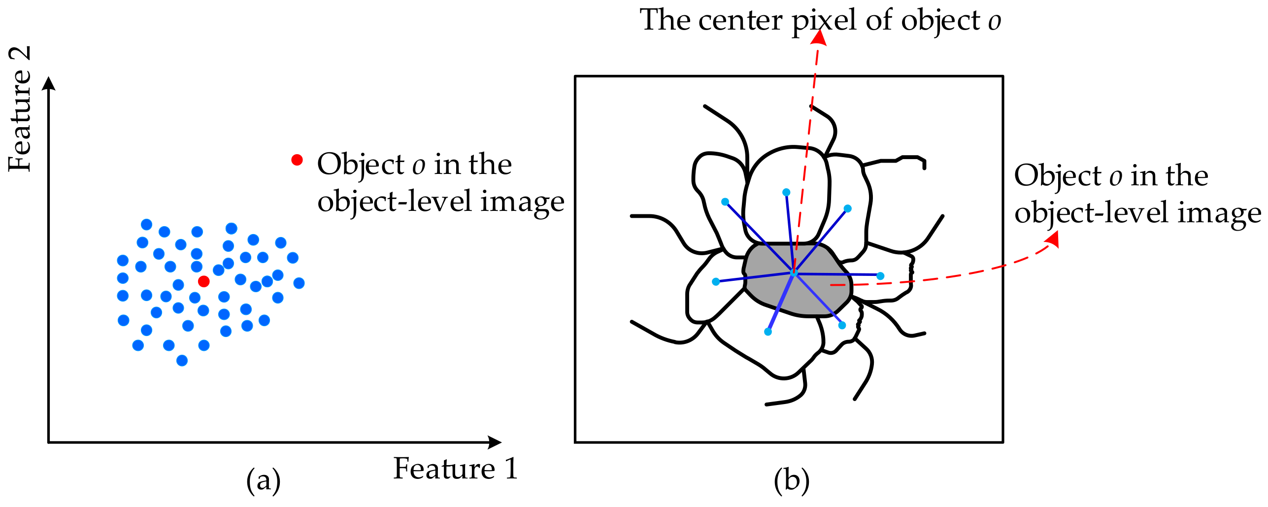
21] only considers a single object, ignoring the dependence between neighboring objects. To overcome this shortcoming, this study proposes a novel higher-order clique potential by constructing a higher-order clique of objects and by considering the dependence between neighboring objects in both feature and location spaces. For a given object
o, its higher-order clique
vo is defined as:
where
o denotes the object
o;
r1(
o) and
r2(
o) denote the two neighboring objects that are nearest to object
o in the feature space; and
g1(
o) and
g2(
o) denote the two neighboring objects nearest to object
o in the location space.
Figure 2a,b shows an example of the feature space (location space) for a simple object-level image.
In order to determine the objects r1(o), r2(o), g1(o), and g2(o), we need to define the distances between objects in the feature and location spaces. For two given objects o1 and o2, their distance in the feature space is defined as the Euclidean distance of x(o1) and x(o2), where x(o1) and x(o2) denote the mean values of the DI features of the pixels in objects o1 and o2, respectively. The distance between o1 and o2 in the location space is defined as the Euclidean distance of the location coordinates of the center pixels of objects o1 and o2.
The clique
vo is made up of three parts: the object
o, its two nearest neighboring objects in feature space, and its two nearest neighboring objects in location space. In general, there is correlation between the neighboring objects—in particular for the over- segmentation objects. The proposed higher-order clique potential function
is defined based on the object clique
vo and is used to utilize the correlation of the pixels within an object and its nearest neighboring objects in both feature and location spaces.
takes the following form:
where
is used to describe the cost of the label inconsistency in the clique
vo.
N(
vo) denotes the number of the pixels in the clique
vo, and consequently, a large clique will have a large weight.
is used to define the cost coefficient, which takes both the clique segmentation quality and the clique likelihood for change/no-change into account. In particular, the cost coefficient
is defined as:
where min represents the minimum operator,
q(
vo) represents the clique segmentation quality of clique
vo, and
zk(
vo) represents the clique likelihood of clique
vo to class
k,
k∈{
Cu,
Cc}.
In this study, the clique segmentation quality,
q(
vo), is defined as the weighted average sum of the segmentation quality of the objects in clique
vo:
where
q(
o),
q(
r1(
o)),
q(
r2(
o)),
q(
g1(
o)), and
q(
g2(
o)) stand for the segmentation quality of objects
o,
r1(
o),
r2(
o),
g1(
o), and
g2(
o), respectively.
Let ol denote a given object in clique vo. Then, the object segmentation quality of ol is estimated based on the object consistency assumption, which encourages all the pixels in an object to have the same class label. Specifically, we define q(ol) as follows: q(ol) = (N(ol) − Nk(ol))/Q(ol), where N(ol) denotes the number of the pixels in object ol, Nk(ol) denotes the number of the pixels assigned to class k in object ol, k∈{Cu, Cc}, and Q(ol) denotes a truncated parameter used to adjust the degree of rigidity of q(ol). This study sets Q(ol) = 0.1 × N(ol). That means, if more than 90% of the pixels in ol are assigned to Cc or Cu, the value of q(ol) is less than 1. Similarly, if 70% of the pixels in object ol are assigned to Cc or Cu, the value of q(ol) is set to 3.
According to the definition of q(ol), the more pixels of an object have the same class label, the better segmentation quality on this object and the smaller value of q(ol) will be. As a result, the better the segmentation quality of the objects in clique vo is, the smaller value of q(vo) will be (see Equation (18)).
The clique likelihood
zk(
vo) is defined based on the number of pixels in the objects from clique
vo and the objects’ joint mass values, taking the following form:
where
N(
o),
N(
r1(
o)),
N(
r2(
o)),
N(
g1(
o)), and
N(
g2(
o)) denote the number of the pixels in objects
o,
r1(
o),
r2(
o),
g1(
o), and
g2(
o), respectively.
mk(
o) denotes the joint mass value of the object
o to class
k and is computed via
mk(
o) =
, where
mi(
k) denotes the joint mass value of pixel
i to class
k,
k∈{
Cu,
Cc}.
mk(
r1(
o)),
mk(
r2(
o)),
mk(
g1(
o)), and
mk(
g2(
o)) have the similar definition of
mk(
o).
Generally, the center object in clique vo is more important than their neighboring objects. Accordingly, when computing q(vo) and zk(vo), the weight of object o is set to 1, whereas the weights of objects r1(o), r2(o), g1(o), and g2(o) are set to 0.5.
On the one hand, the proposed higher-order clique potential encourages all pixels in clique vo to have the same class label. On the other hand, it uses the label consistency in a clique as a soft constraint and, thus, enables some pixels in the clique to take different labels. Accordingly, the higher-order clique potential can make effective use of the interaction of the pixels within an object and its nearest neighboring objects in both feature and location spaces and, thus, can improve the CD performance.
Different optimization algorithms, such as graph cuts and iterated conditional modes, can be adopted to minimize (optimize) the CRF model. The graph cut algorithm [
33] is used to minimize the HOC
2RF model for producing the final CD map.


