Abstract
In this study, we investigate sea state estimation from spaceborne GNSS-R. Due to the complex scattering of electromagnetic waves on the rough sea surface, the neural network approach is adopted to develop an algorithm to derive significant wave height (SWH) from CYGNSS data. Eighty-nine million pieces of CYGNSS data from September to November 2020 and the co-located ECMWF data are employed to train a three-hidden-layer neural network. Ten variables are considered as the input parameters of the neural network. Without the auxiliary of the wind speed, the SWH retrieved using the trained neural network exhibits a bias and an RMSE of −0.13 and 0.59 m with respect to ECMWF data. When considering wind speed as the input, the bias and RMSE were reduced to −0.09 and 0.49 m, respectively. When the incidence angle ranges from to and the SNR is above 7 dB, the retrieval performance is better than that obtained using other values. The measurements derived from the “Block III” satellite offer worse results than those derived from other satellites. When the distance is considered as an input parameter, the retrieval performances for the areas near the coast are significantly improved. A soft data filter is used to synchronously improve the precision and ensure the desired sample number. The RMSEs of the retrieved SWH are reduced to 0.45 m and 0.41 m from 0.59 m and 0.49 m, and only 16.0% and 14.9% of the samples are removed. The retrieved SWH also shows a clear agreement with the co-located buoy and Jason-3 altimeter data.
1. Introduction
Significant wave height (SWH) is important for ocean applications, such as climate evaluation and ocean engineering. Precisely monitoring and forecasting it is critical. Buoys, which can provide the most comprehensive information, are a traditional tool used to measure SWH [1]; however, their spatial coverage is severely limited. Furthermore, they are too expensive to widely distribute. Spaceborne altimeters, as an important remote sensing technology, can globally measure SWH. The typical representatives are Topex-Poseidon [2], Jason [3], HaiYang2 (HY2) [4], and the Satellite for ARgos and ALtika (SARAL/Altika) [5]. Spaceborne altimeters provide accurate measurements along the “nadir” track, as well as kilometer-level spatial resolution; however, they have a low temporal resolution. Spaceborne synthetic aperture radars (SARs), such as Envisat [6], Sentinel-1 [7], and Gaofen-3 [8], are also useful for monitoring ocean waves. It was found that the root mean square (RMS) of the signal-to-noise ratio (SNR) from SAR images has a linear relationship with the SWH [9]. Unfortunately, wave measurements from SAR are low-density. Scatterometers are designed to measure sea wind vectors with a spatial resolution of about 25 km and a precision of 2 m/s. Scatterometers can monitor oceans with a high revisit frequency. The Advanced Scatterometer (ASCAT) on board the MetOp-A satellite covers the global ocean in 1.5 days, and the Quick Scatterometer (QuickSCAT) covers 90% of the global ocean each day. The primary objectives of scatterometers are to measure ocean wind vectors; however, they also have the ability to measure SWH. In [10,11], the data from the Earth Remote Sensing Satellite-1/2 (ERS-1/2) and Quick Scatterometer (QuickSCAT) were used to retrieve SWHs based on an artificial neural network. A multi-layer neural network was trained to derive SWHs from ASCAT data, and the results showed that under moderate sea conditions (1.0–5.0 m), the SWH from the multi-layer network and the WaveWatch III had a root mean square error (RMSE) of 0.5 m [12]. A deep neural network was developed to combine the data from the Surface Waves Investigation and Monitoring (SWIM) instrument and the China–France Oceanic SATellite (CFOSAT) to retrieve SWHs over an extended swath, and a RMSE of 0.26 m was obtained [13]. Some other wave radars were also used to retrieve SWH, such as high-frequency (HF) radars [14].
Global Navigation Satellite System-Reflectometry (GNSS-R) is a new remote sensing tool that synchronously receives the direct GNSS signal and the corresponding signal reflected off the Earth’s surface to retrieve the Earth’s physical parameters, such as wind fields [15,16], sea surface height [17,18], sea ice [19,20], soil moisture [21,22], etc. Some spaceborne GNSS-R missions, such as the UK TechDemoSat-1 [23], Cyclone GNSS (CYGNSS) [24], and Bufeng [25], have provided global observations of Earth’s parameters. For GNSS-R, the interferometric complex field (ICF) [26] and interference pattern technique (IPT) [27] were proposed to measure SWH in coastal scenarios. These two methods are both based on the coherence of the reflected signal being dependent upon the sea state. Unfortunately, for most spaceborne cases, the coherence of the signal reflected off the sea surface is extremely weak [28], so they fail to work in spaceborne cases. It was demonstrated that the whole delay-Doppler maps (DDMs) from the UK DMC satellite were potentially able to improve the observations of wind and waves [29]. The sensitivity of the reflected GNSS signal to wave was noticeable at wind speeds ≤10 m/s [30]. It was found that SWH had a strong effect on the defined Scaled SNR (SSNR) of the DDM [31]. In [32], the observable in [9] was extended to the CYGNSS data to measure SWH. These works indicated that GNSS-R can be used to improve the understanding of surface waves.
Artificial intelligence methods have been widely used to retrieve the Earth’s physical parameters and obtained better retrieval performances than the analytical functions [33]. They have also been used in spaceborne GNSS-R [34,35,36]. In this study, to demonstrate the potential of spaceborne GNSS-R for monitoring sea waves, a novel approach for measuring SWH from the CYGNSS data is developed. It is found that the SWH from the CYGNSS data is in agreement with the re-analyzed ECMWF, co-located buoys, and Jason-3 altimeter data. Section 2 describes the data from the CYGNSS, ECMWF, buoys, and Jason-3 altimeter. Section 3 discusses the wind–wave relationship. The architecture and training process of the neural network are described in Section 4. The SWHs from the CYGNSS data and the ECMWF are compared in Section 5. Section 6 gives an approach to improve the retrieval precision of the SWH. Section 7 presents the comparison of the retrieved SWH with the buoy and Jason-3 SWHs. The discussion and conclusion of this paper are addressed in Section 8 and Section 9.
2. Data
2.1. CYGNSS Data
The primary objective of the CYGNSS is to retrieve sea wind speed with a low mission cost. The CYGNSS constellation consists of eight micro-satellites with a weight of about 17.6 kg. The orbit inclination and altitude are and 500 km, respectively. Each satellite simultaneously samples the quasi-specular scattered signals from up to four available GPS transmitters. The spatial resolution and the mean revisit time are 25 km and 7 h, respectively [37]. A detailed mission description was provided in [38,39].
The basic observable of spaceborne GNSS-R is the DDM, which describes the distribution of the correlation power in the two-dimensional delay and Doppler domain. The DDM size for the level 1 (L1) data of the CYGNSS is 17 × 11. The delay and Doppler resolution are 0.25 chips and 500 Hz, respectively [40]. From the DDM, the features sensitive to Earth’s physical parameters, such as the normalized bi-static radar cross section (NBRCS) [40] and leading edge slope (LES) [41], are defined. The CYGNSS data used in this paper are L1 version 3.0 data, which were downloaded from http://doi.org/10.5067/CYGNS-L1X30, accessed on 23 July 2021. The data not only consist of the NBRCS and LES but also include a series of geometry and instrument parameters at the acquisition time. The data from September to November 2020 are used to retrieve SWH and evaluate the performance. The DDM with the SNR less than 2 dB is removed to ensure the used DDM are of good quality. The definition of the DDM SNR can be found in [32].
2.2. ECMWF
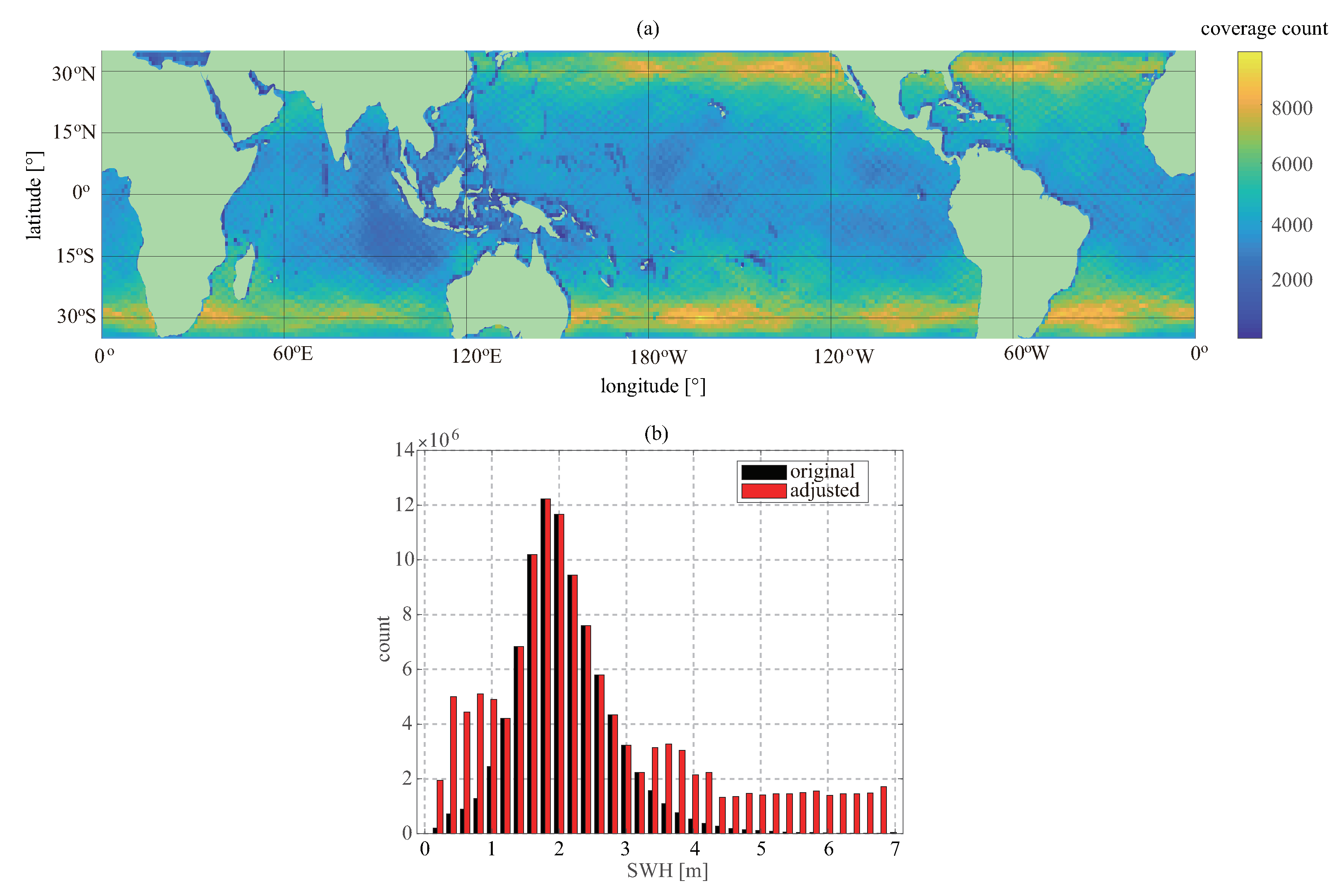
The SWH and wind speed from ECMWF ERA5, which were downloaded from https:cds.climate.copernicus.eu/cdsapp#!dataset/reanalysis-era5-single-levels?tab=from, accessed on 23 August 2021. are used to develop and evaluate the model of retrieving SWH. The ECMWF provides the global and hourly estimations of many atmospheric, land, and oceanic climate variables. The wind speed and SWH have a spatial resolution of 25 km and 50 km, respectively. The ECMWF data have to be collocated with the CYGNSS data. In time dimension, the maximum temporal offset is 0.5 h. In space, a two-dimensional linear interpolation is used to obtain the co-location wind speed and SWH. The match-up process yields a dataset more than 11 million data pairs. The specular points of the CYGNSS in the matched dataset are shown in Figure 1a, which cover a latitude from N to S. There are more measurements in the latitude of than other latitudes due to the orbit inclination of the GYGNSS satellite. The tracks of the CYGNSS sub-satellites have more measurements than other regions. Figure 1b shows the distribution of the SWH in the match-ups. Most SWHs range from 0 to 7 m, and only a few samples are at 0∼1 m and 4∼7 m. This distribution may cause low accuracy at the low and high SWH due to the under-fitting. This phenomenon, known as the sample imbalance problem, is common in machine learning (ML). To decrease the risk of the under-fitting caused by an imbalanced sample, sample balancing is carried out. A widely used method is the oversampling technique. Here, a simpler method, replicating the samples from the minority [42], is used. This procedure involves repeatedly copying the match-ups when the match-up number is located in a given interval as follows:
where is a unit row vector; ⊗ represents the tensor product operator; and is a row vector which is composed of the SWHs from and . In this paper, the SWHs in the match-ups are divided into 35 groups, and is . For the SWH group , can be computed as:
where is the maximum operator; is the size of ; and is a fractional value which is 1 for , 0.35 for and , 0.30 for and , 0.25 for and , and 0.15 for . The red histogram in Figure 1b shows the distribution of the adjusted SWH, in which the numbers of the samples at the low and high SWHs are effectively improved. This improvement reduces the risk of under-fitting at the low and high SWHs.

Figure 1.
(a) Trajectory of specular points of CYGNSS; (b) distribution of SWH in matched dataset.
All match-ups are randomly split into two groups: the training and test set. The training set, which has 1.30 million match-ups, is used to develop the neural network. The test set serves to evaluate the performance of the neural network.
2.3. Buoy
The hourly SWHs from the buoy network of the National Data Buoy Center (NDBC) are collected to evaluate the precision of the retrieved SWH. The chosen buoys are depicted in Figure 2. They are mainly moored off Hawaii, the Gulf of Mexico, and the east coast of North America. The thresholds for the temporal and spatial associations between the retrieved SWH and the buoy are 30 min and 25 km. In total, 4600 match-ups are collected. To ensure the independence of the comparison between the retrieved SWH and buoy data, the buoy match-ups are not used to develop the neural network.
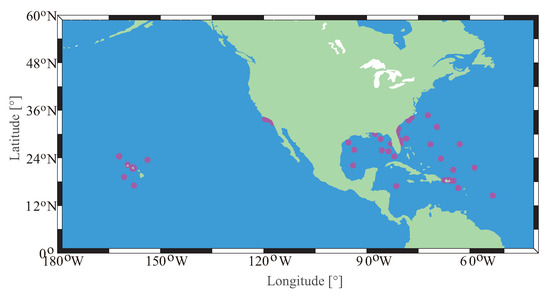
Figure 2.
Locations of the NDBC buoys used in this study.
2.4. Jason-3 Altimeter
Jason-3 is the fourth mission of a series of US–European satellite missions, which has a non-sun-synchronous orbit with an altitude of 1336 km, an inclination of , and a cycle of about 9.5 days [43]. The primary task is to measure global sea-level variation and SWH using a Ku-band and C-band altimeter. The measured SWH, which is downloaded from http://www.ncei.noaa.gov/data/oceans/jason3/gdr_f/gdr, accessed on 21 March 2022, is used to evaluate the retrieved SWH. The spatial and temporal gaps between the Jason-3 data and CYGNSS observation are 30 min and 25 km, respectively. About 193,000 match-ups in total are collected.
3. Wind–Wave Relationship
The SWH mainly consists of wind-driven and swell-driven SWH. For a fully developed sea, according to the Pierson–Moskowitz spectrum, wind-driven SWH is approximately expressed as [44]:
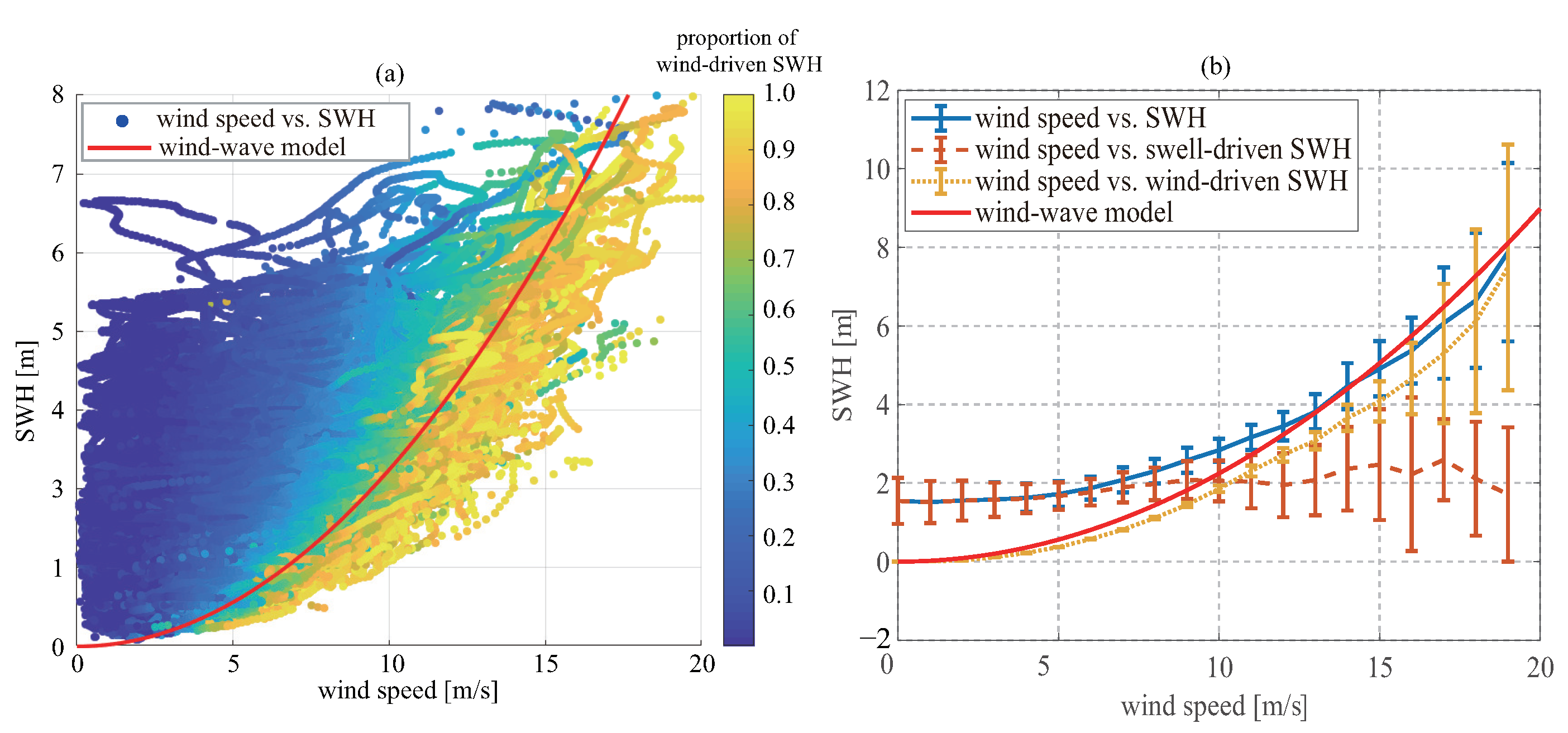
where is the 10 m wind speed, and g is the gravity acceleration. The ratio between wind-driven SWH and total SWH is defined to evaluate the impact of wind speed on SWH. As shown in Figure 3a, some SWHs exhibit the correlation relationship with wind speeds, the ratios of which are closer to 1; however, a large number of points deviate from the Equation (3), and the deviation becomes serious as wind speed decreases. The means and standard deviations of swell-driven, wind-driven, and total SWHs at different wind speeds are presented in Figure 3b. When wind speed is below 5 m/s, the statistics of total SWH agree with these of swell-driven SWH. As wind speed increases, the statistics of total SWH gradually break away from these of swell-driven SWH, but tend to the statistics of wind-driven SWH. This indicates that the dominant driving force of sea wave at low wind speed is swell, whereas at high wind speed, the driving force is wind speed. The response of the GNSS-R dominates the specular or quasi-specular scattering [45], which is mainly determined by the large-scale roughness. For a given surface height spectrum, the cut-off wavelength separating the large and small-scale roughness is [46]:
where is the GNSS signal wavelength and is the incidence angle of the GNSS signal. When the signal is normally incident, the cut-off wavelength is minimal. For the GPS L1, L2, and L5 signals, the minimum cut-off wavelengths are about 57, 73, and 77 cm, respectively; therefore, the wave longer than 60 cm is sensed by GNSS-R. The swell-driven spectrum lies at the ∼100 m scale. This indicates that wind speed and swell both contribute to the reflected GNSS signal. A significant dependence of GNSS-R observable in the swell was observed at wind speeds <6 m/s [30].

Figure 3.
(a) Scattering between SWH and wind speed from ECMWF and (b) statistical features of SWH versus wind speed.
4. Neural Network
GNSS-R measurement depends on wind and swell, but there is no explicit relationship among them. It is difficult to obtain an analytical expression due to a complex interaction mechanism between the GNSS signal and rough sea surface, and a dynamic geometry among GNSS satellite, low earth orbit (LEO) satellite, and specular point. Here, a neural network is used to develop the complex relationship of GNSS-R measurement with SWH and GNSS-R geometry parameters.
4.1. Architecture
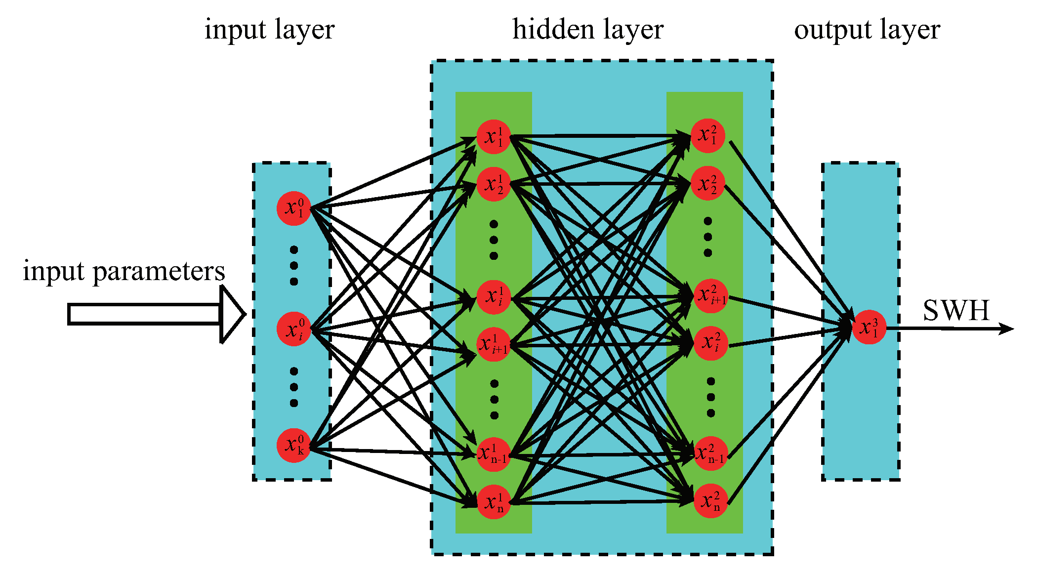
Many neural networks were proposed to explore the complex relationships. As shown in Figure 4, a multi-layer feed-forward neural network is used to develop the retrieval model of SWH, in which the input parameters are the GNSS-R measurements and geometry parameters, and the output is SWH. The hidden layer number and the neuron number in each hidden layer are properly chosen to obtain a good retrieval performance. The usual transfer functions in a neural network are the sigmoid, hyperbolic tangent, and rectified linear function (RELU):

Figure 4.
Architecture of the neural network used in this study.
4.2. Input Analysis
The basic GNSS-R measurements of the CYGNSS contain the NBRCS, LES, and SNR, which are widely used to retrieve wind speed [47]. Therefore, the NBRCS, LES, and SNR are considered as the input parameters for the first case. The incidence angle of the GNSS signal, the antenna gain at a specular point (sp_rx_gain), and GNSS PRN have important effects on retrieval performance [47,48]; therefore, the input parameters for the second case also contain the sp_rx_gain, incidence angle, azimuth angle, and PRN. Swell and wind wave zone shows a significant spatial pattern [49,50]. For a nearshore areas, coastal topography and coastline orientation also affect sea wave. It is useful to consider the geographical information in a spaceborne algorithm. The latitude and longitude of the specular point (spLat, spLon) were used to improve the GNSS-R retrieval precision [35,51]. The offshore wave is not only influenced by wind speed and swell, but also affected by the shoaling, refraction, and diffraction of seabed [52]. It is difficult to obtain the water depth at a specular point, so the distance from the specular point to the coastline (distance) is used to replace the water depth. The third case is generated by adding the above three geographical parameters into the second case. Wind speed is a driving force of wave, especially at high wind speed; hence, based on the third case, wind speed is considered as an input in the fourth case. The inputs of the neural networks are listed as follows:
- Case 1: NBRCS; LES; SNR;
- Case 2: NBRCS; LES; SNR; sp_rx_gain; incidence angle; azimuth angle; PRN;
- Case 3: NBRCS; LES; SNR; sp_rx_gain; incidence angle; azimuth angle; spLon; spLat; distance;
- Case 4: NBRCS; LES; SNR; sp_rx_gain; incidence angle; azimuth angle; spLon; spLat; distance; wind speed.
Here, a two-hidden layer neural network is used to evaluate the retrieval performance of the four cases. The transfer functions in the hidden and output layer, respectively, adopt the hyperbolic tangent and RELU. The neuron number in each hidden layer is 25. Table 1 shows the SWH retrieval performance for each case. The first case is considered as the baseline to compare with the other cases. When the antenna gain, incidence angle, azimuth angle at specular points, and PRN are considered as the input, the bias and RMSE are reduced by 40.54% and 13.68%, respectively. For the third case, because the geographical parameters are added into the input, the bias and RMSE are further reduced by 40.91% and 28.05%, respectively. This indicates that the geographic parameters provide extra information for the neural network. When wind speed is added to the neural network, compared to the third case, reductions of 30.77% and 16.95% in bias and RMSE are obtained, respectively. The first, second, and third cases represent the independent retrieval using only CYGNSS data. The fourth case combines the CYGNSS data and auxiliary data to retrieve SWH. In the following, the third and fourth cases are used to retrieve SWH and evaluate the retrieval performance.

Table 1.
The performance of each input parameter combination.
4.3. Architecture Optimization
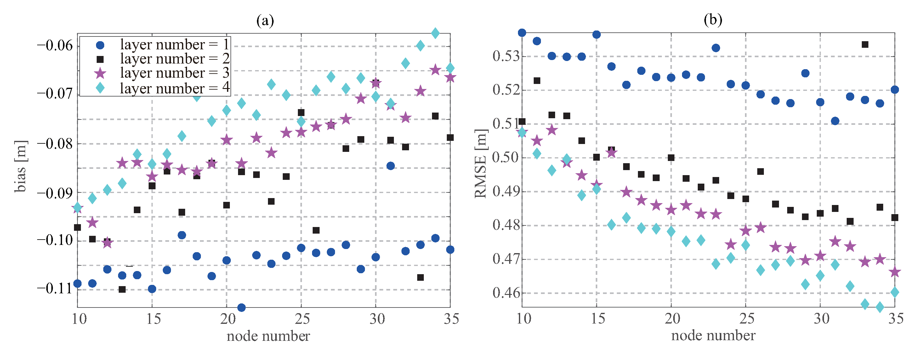
The ability to approximate a nonlinear function depends on the neuron number in the hidden layers and the transfer functions. The optimal neuron number in the hidden layers and the combination of the transfer functions in the hidden and output layers have the smallest bias and RMSE. When the PELU, which allows a wider output range than the other two functions, is used as the transfer function in the output layer, a better performance is obtained. For the transfer functions in the hidden layers, the test results of the hyperbolic tangent function are better than those of the sigmoid and PELU functions. Therefore, the hyperbolic tangent and PELU functions are adopted in the hidden and output layers, respectively. Figure 5 shows the bias and RMSE of the retrieved SWH for the different hidden layer number and the neuron number in each hidden layer. The bias and RMSE both decrease as the neuron number increases; however, once the neuron number is above 30, the bias and RMSE tend to be stable. Hence, in the hidden layers, 30 neurons are considered as the optimal configuration. The neural networks with three and four hidden layers exhibit a similar retrieval performance and have better retrieval performance than these with one and two hidden layers. Therefore, the neural networks in this paper contain three hidden layers.
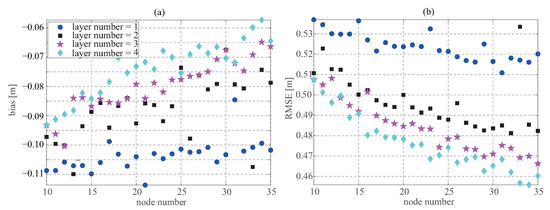
Figure 5.
(a) Bias and (b) RMSE values for different numbers of hidden layers and numbers of neurons in each hidden layer.
5. Evaluation of Retrieved SWH
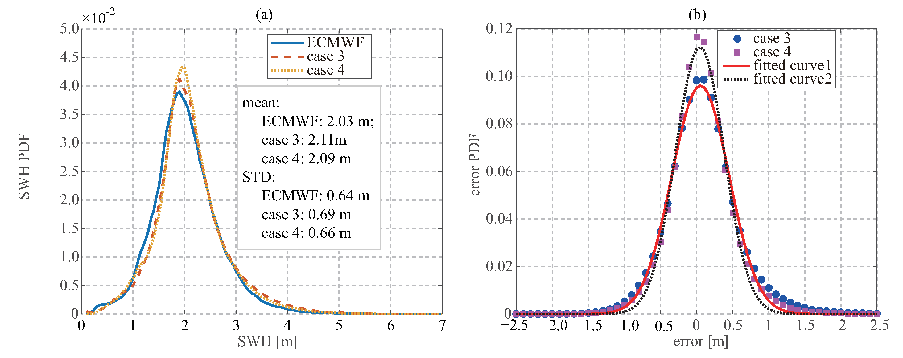
Figure 6 shows the comparison of the retrieved SWH against ECEMF data. Most data pairs are centered around the 1:1 line; however, the two-side distributions of the 1:1 line are unsymmetrical. This indicates that there are positive or negative biases at different SWHs. The fourth case shows an overall better performance than the third case. When wind speed is not the input, the bias and RMSE of −0.13 and 0.59 m are obtained, and when wind speed is considered as the input, the bias and RMSE are −0.09 and 0.49 m, respectively. As shown in Figure 7a the PDFs of the retrieved SWH and ECEMF data both range from 0 to 7 m, and the most are from 1 to 3 m. As presented in Figure 7b, the errors of the third and fourth case are centered around zero, and the probabilities of the absolute error above three standard deviations are 6.05% and 4.36%, respectively.
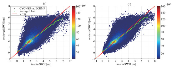
Figure 6.
Scatter between retrieved SWH and ECMWF data for (a) the third case and (b) the fourth case.
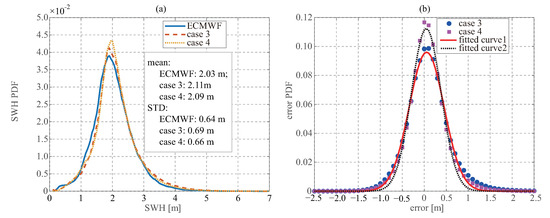
Figure 7.
Probability density functions of (a) the retrieved SWH and ECMWF data and (b) error between the retrieved SWH and ECMWF data.
5.1. Dependence on SWH
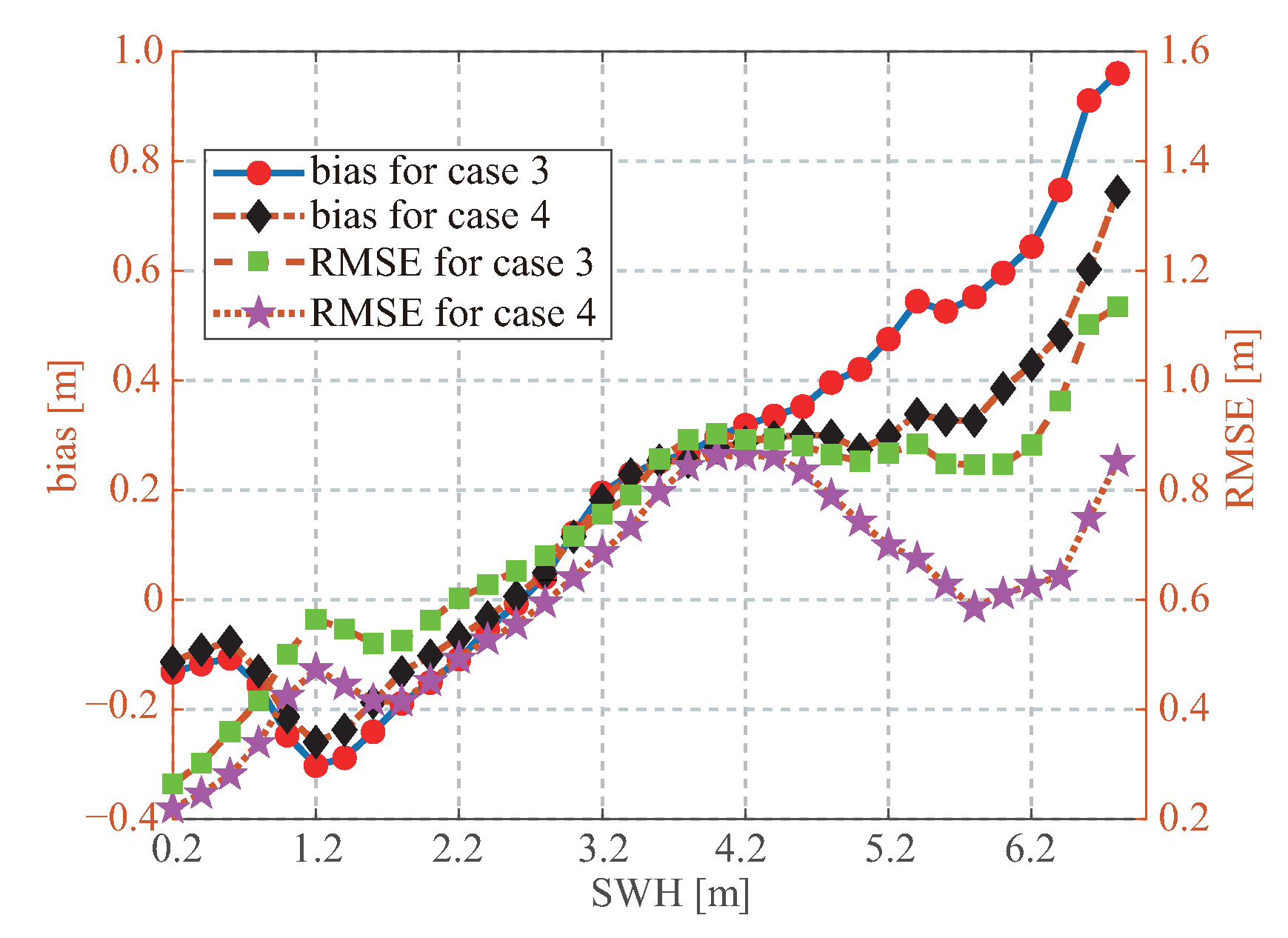
As shown in Figure 6, the asymmetries of the data pairs around the 1:1 line are obvious and different at different SWHs. Figure 8 shows the biases and RMSEs at different SWHs. When SWH is below 2.5 m, the retrieved SWH has a negative bias; however, for the SWH above 2.5 m, the bias becomes positive. The RMSE of the SWH from 2.5 to 5.0 m, where the impact of wind speed and swell on sea wave are equivalent, is larger than that of the SWH below 2.5 m, where the dominant wave comes from swell. The neural networks are underestimated for the SWHs below 0.5 m and above 6.5 m due to few match-ups, so the RMSEs rebound. The retrieval performances of the fourth case outperform those of the third case, especially at high SWH, where wind-induced SWH dominates sea wave. This indicates that when wind- or swell-induced SWHs dominate sea wave, the neural networks provide better retrieval performance.
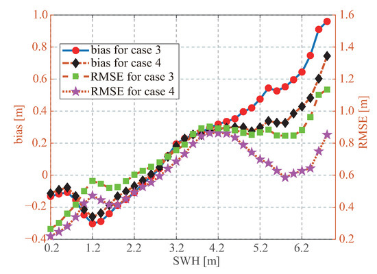
Figure 8.
Biases and RMSEs compared between the retrieved SWH and ECMWF data at different SWHs.
5.2. Dependence on Incidence Angle
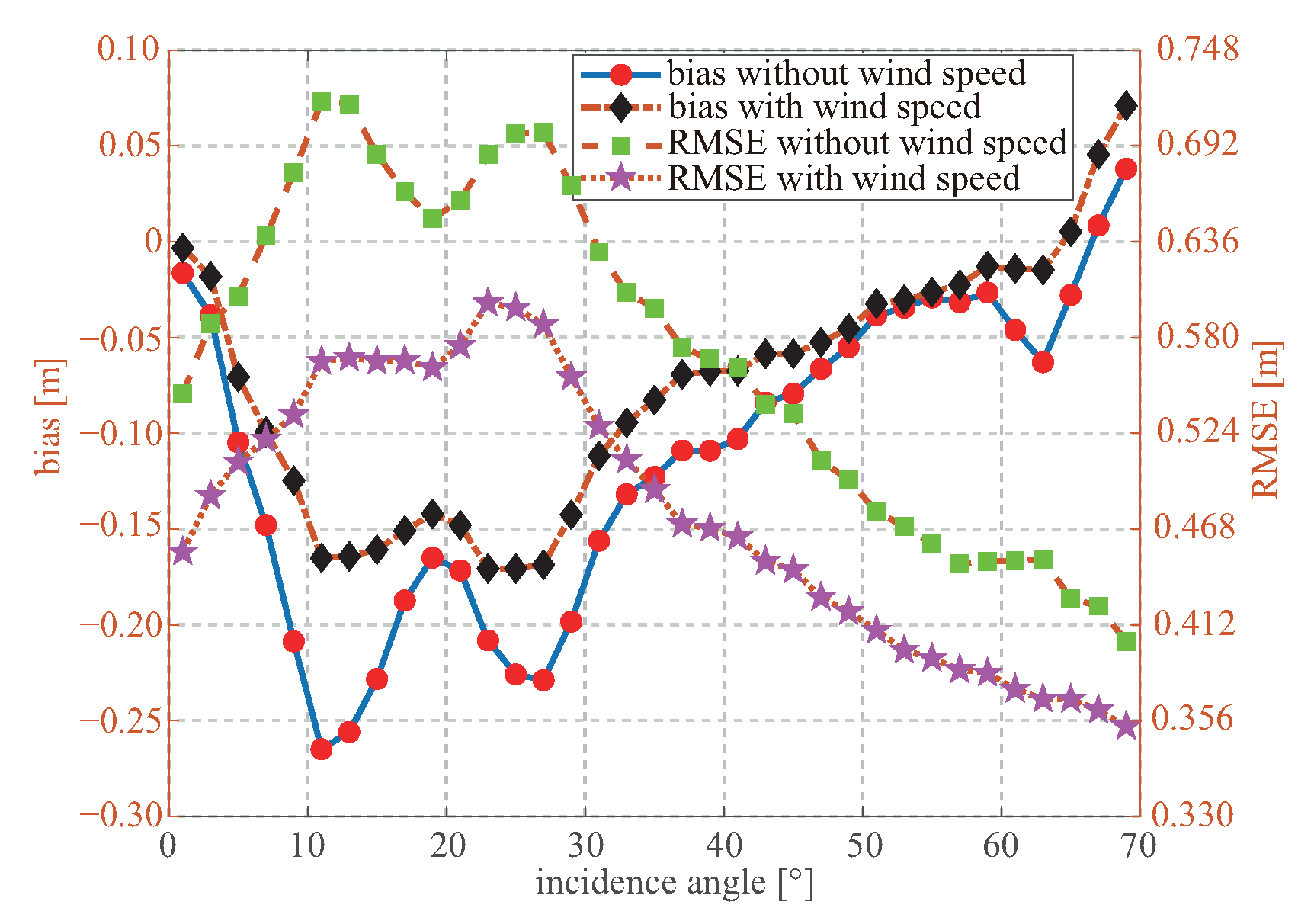
The dependence and importance of the incidence angle on the retrieval performance of wind speed were demonstrated in [30,47,48,49,51]. The incidence angle of the CYGNSS data mainly ranges from to , and 80.5% of the data have an incidence angle of 20∼60. Figure 9 shows the biases and RMSEs at different incidence angles. The results with the incidence angle from to are better than these of the other incident angles. At the incidence angle below and above , the retrieval performance is statistically insignificant and meaningless as the data in these bins are not sufficient.
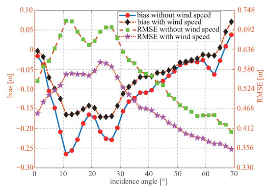
Figure 9.
Biases and RMSEs between the retrieved SWH and ECMWF data at different incidence angles.
5.3. Dependence on SNR
Intuitively, the higher the SNR, the better the data quality, and the better the retrieval performance. Figure 10 shows the bias and RMSE of the retrieved SWH versus the SNR. The bias changes from negative to positive, and the absolute bias at high SNR is better than that at low SNR. The RMSE presents a falling trend as the SNR increases and gradually tend to be stable once the SNR is above 7 dB. The main GNSS-R measurement is the NBRCS, which is estimated from the received power. The standard deviation of the received power explains the changing phenomenon of the RMSE. The standard deviation of the received signal is given as [53]:
where N is the incoherently averaged number and is the mean of the receiver signal power. After a certain value, increasing SNR will not significantly reduce the standard deviation of the received power, so cause a limited improvement in retrieval performance.
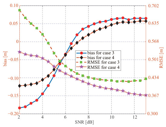
Figure 10.
Biases and RMSEs between the retrieved SWH and ECMWF data at different SNR.
5.4. PRN
The GPS constellation includes 8 Block IIR (“Replenishment”), 7 Block IIR-M (“Modernized”), 12 Block IIF (“Follow-on”), and 4 GPS III/IIIF. GPS satellites in distinct blocks have different signal levels and angular gain distributions [54]. In [55], it was found that PRN is the fifth-most dominant feature for the retrieval of wind speed. The dependence of wind speed retrieval performance on GPS block types was also validated in [56]. These results indicate that the GPS block type has an important influence on the retrieval performance. As shown in Figure 11, the SWHs from the PRN 24, 4, and 15 satellites with the block types of IIF, IIR-M, and IIR-M present worse performance. It should be noted that there are no match-ups from PRN 14, 18, and 23 satellites. As shown in Table 2, the poorest and best performance of the retrieved SWH are from Block IIR and III/IIIF satellites, respectively.
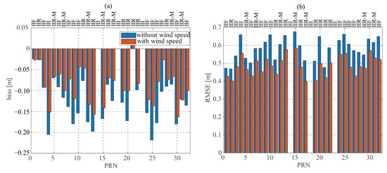
Figure 11.
(a) Biases and (b) RMSEs between the retrieved SWH and ECMWF data at different GPS PRN values.
Table 2.
Retrieval performance for different block-type satellites.
5.5. Spaceborne ID
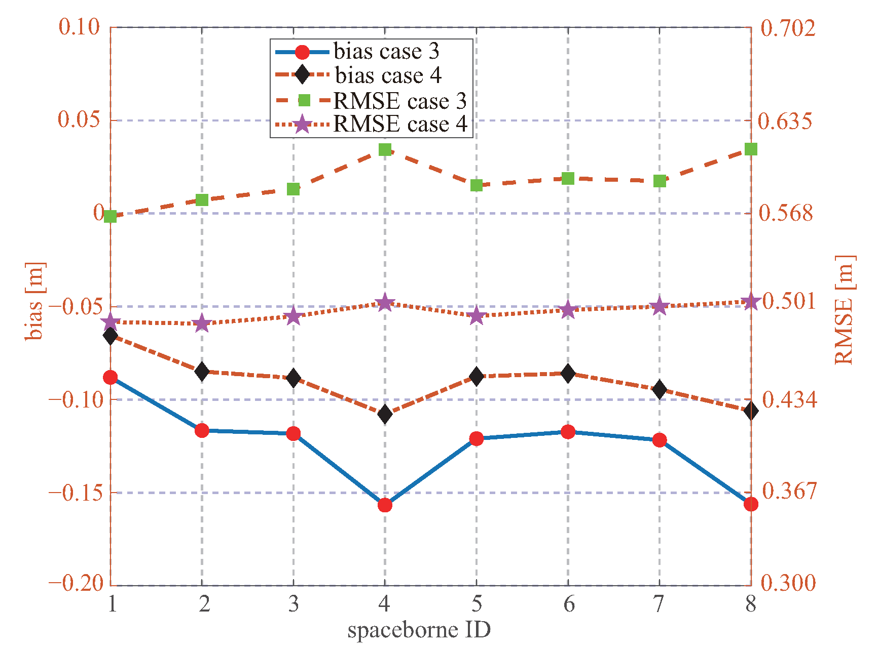
There was a non-negligible inter-satellite bias between the CYGNSS spacecrafts [57]. This indicates that the CYGNSS L1 observable depends on the individual CYGNSS spacecraft. This bias was found in the v2.0 CYGNSS data, and several calibrations were changed in the v3.0 version; however, the inter-satellite bias may still be present in the v3.0 version. As shown in Figure 12, regardless of the case 3 and case 4, the retrieved SWHs from the platform 4 and 8 are worse than those from the other platforms. This indicates that the inter-satellite difference result in the different performance in the SWHs retrieved from individual spacecraft.
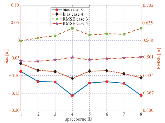
Figure 12.
Biases and RMSEs between the retrieved SWH and ECMWF data for different spcaeborne platforms.
5.6. Distance to Coast
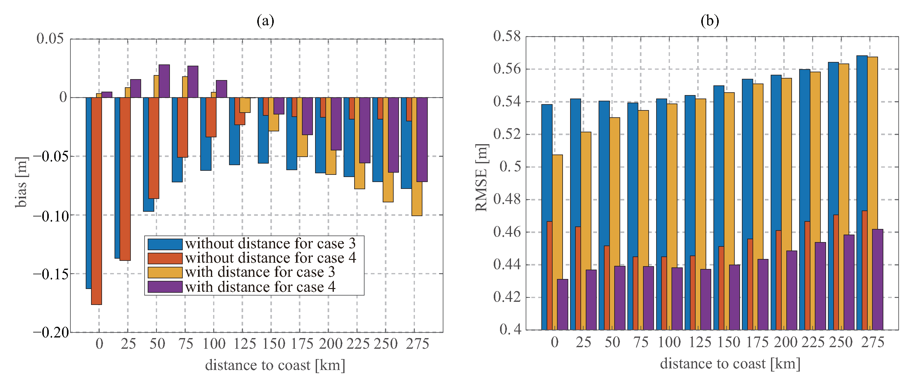
The distance from the specular point to the coastline is also considered as an input of the neural network. The GNSS-R observable near the coastline are strongly affected by the land and near-shore shallow water. Furthermore, the coastal topography and seabed also have important effects on sea wave. Figure 13 presents the bias and RMSE of the retrieved SWH versus the distance to the coastline. When the distance is not the input of the neural network, as the observation region is far away from the land, the performances of the retrieved SWH for the third case become better; however, once the distance exceeds 125 km, they gradually worsen. When the distance is the input, the retrieval performances near the coastal region significantly improved.
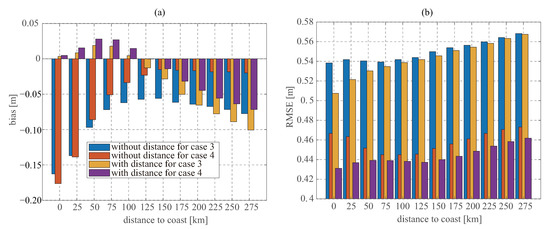
Figure 13.
(a) Biases and (b) RMSEs between the retrieved SWH and ECMWF data at different distances from the specular point to the coastline.
5.7. World Analysis
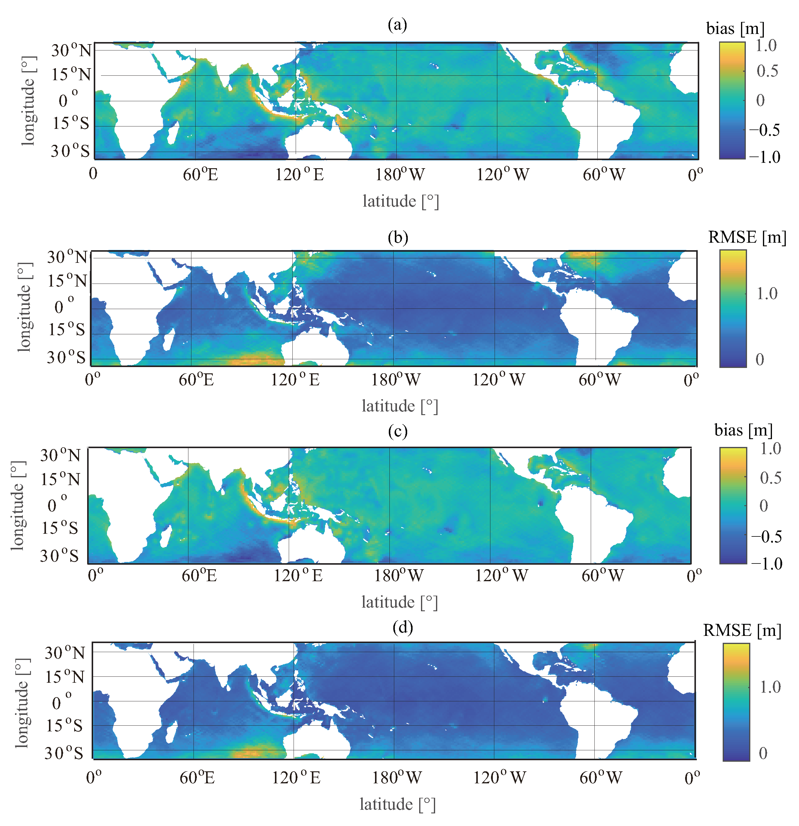
Figure 14 shows the global distribution of the biases and RMSEs of the retrieved SWHs, in which the grid size in latitude and longitude is . The global maps of the biases indicate that the neural networks perform well in most regions where the biases are around 0, whereas large positive biases occur along the coastline of the west Pacific and northeast Indian Oceans. The global maps of the RMSEs indicate that the retrieved SWHs show worse performance in high-latitude regions than in low-latitude regions.
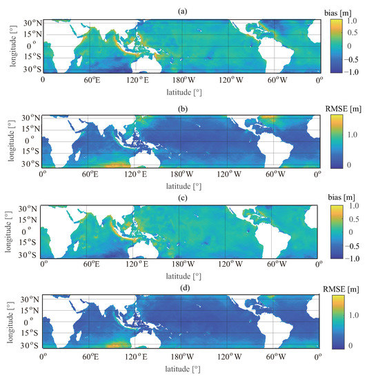
Figure 14.
Illustration of global monthly gridded retrieval performance maps. (a) Gridded biases and (b) RMSEs when wind speed was not considered as an input parameter; (c) gridded biases and (d) RMSEs when wind speed was considered as an input parameter.
6. Improving Precision
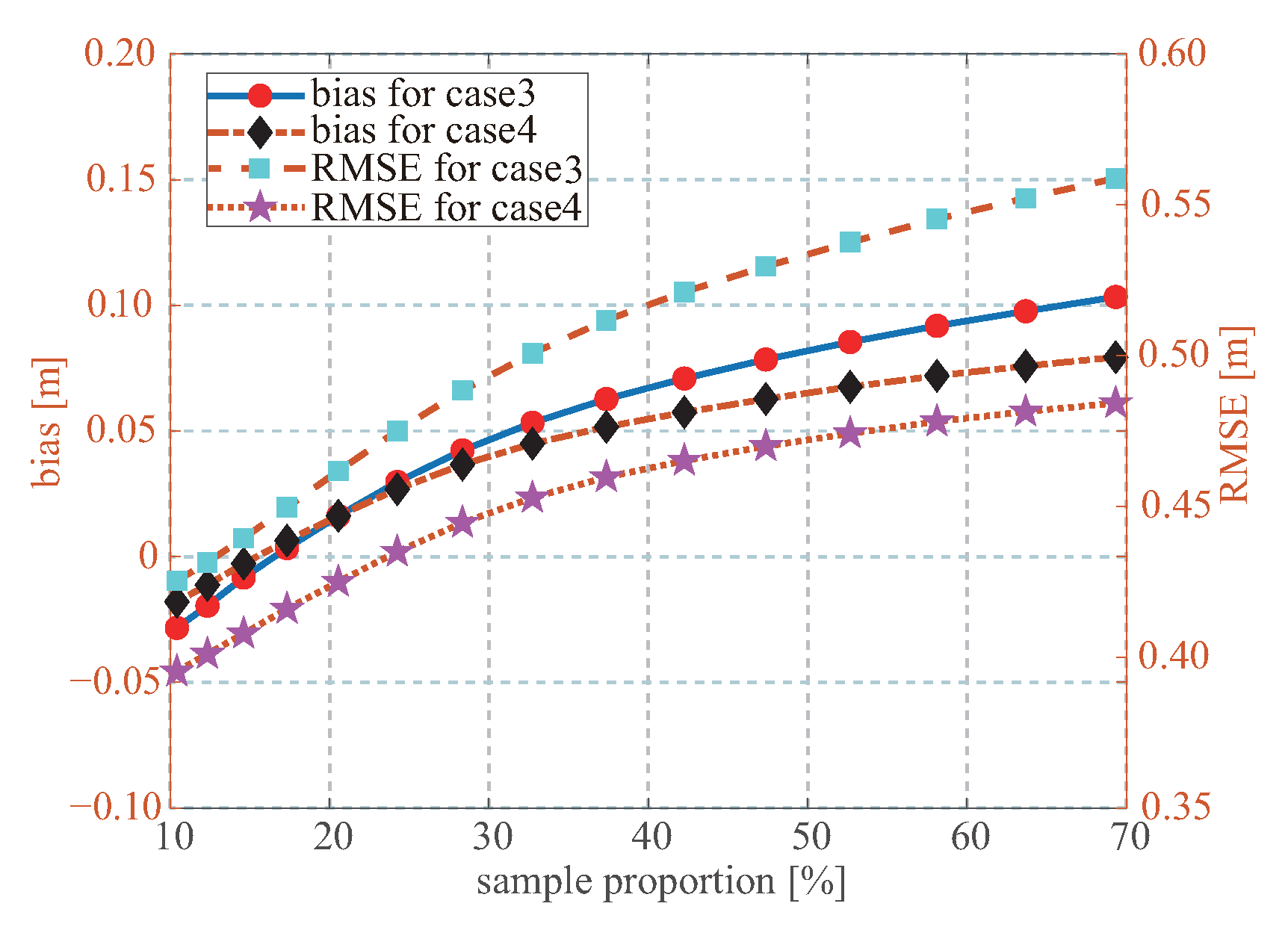
The retrieval performances with the incidence angle from to and the SNR above 7 dB are better than those with other values. The GNSS-R measurements from PRN 24, 4, and 15 satellites are worse than those from other GPS satellites. To further improve the retrieval performance, a feasible approach is quality control through limiting the incidence angle, SNR, and PRN within the optimal ranges. After the quality control, for the third and fourth case, the RMSEs are reduced by 32.20% and 26.53%, respectively. Although the retrieval performances are improved, about 96.3% of the data are removed. As shown in Figure 15, the retrieval performances and the match-up percentage present inversely proportional relationships. A low quality control is important for the application with a good spatial and temporal sampling, whereas a high quality control is important for the application with a low-uncertainty SWH.
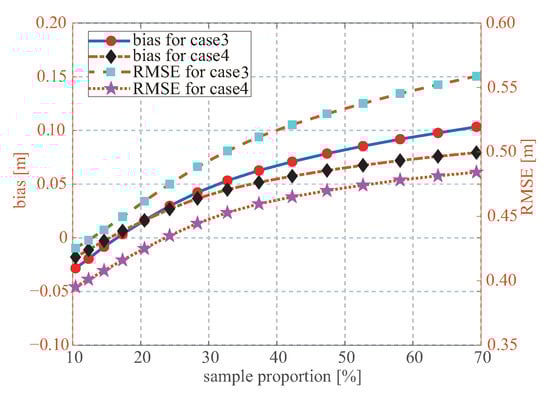
Figure 15.
Biases and RMSEs of ANN-based SWHs versus sample percentage.
The threshold method is a rigid quality control, which may filter out a large number of high-quality data. A soft quality control based on the neural network is developed to effectively identify the outlier, such as the method proposed in [55]. Data with the absolute error larger than 1 m is defined as the outlier. The adopted neural network is also shown in Figure 4. Because identifying the outlier is a classification problem, the transfer function in the output layer is replaced by the hyperbolic tangent function. The outlier and good data are represented as “0” and “1”, respectively. The confusion coefficients of the test are presented in Table 3. The true positive and true negative ratios of the third and fourth case are beyond 88% and 67%, respectively. Correspondingly, the correction rates for the third and fourth case are 86.9% and 87.2%, respectively.
Table 3.
Confusion coefficients for neural network classifier.
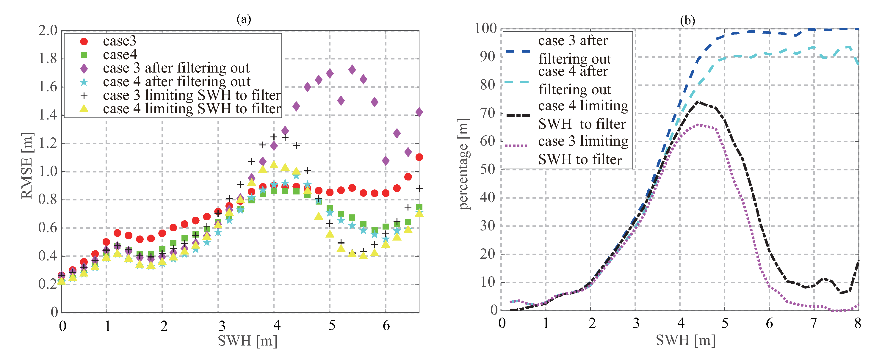
After removing these identified outliers, the RMSEs are reduced by 23.7% and 18.4% to 0.45 m and 0.40 m for the third and fourth case, respectively. Only 16.0% and 14.9% of the samples are filtered out, which are far less than 84.8% and 89.0% of the threshold method. This means that designing and developing a soft data filter is far more significant than the simple threshold method to improve the retrieval performance. As shown in Figure 16a, when the SWH is below 3.5 m, the retrieval performances for both the third and fourth case are significantly improved after the identified outliers are filtered out. Once the SWH is beyond 3.5 m, an increase in RMSE is observed for the third case. The main reason is that a large number of the retrieved SWHs which have good consistencies with ECMWF data are removed, and some SWHs around the regression line are identified as the good-quality samples and retained. As shown in Figure 16b, as the SWH increases, the more samples are identified as the outliers and removed. Specifically, for the SWH greater than 5 m, more than 90% of the samples are filtered out. For the fourth case, there is no prominent increase for the SWH greater than 5 m. The main reason is that wind-induced SWH dominates the total SWH over 5 m, and wind speed plays a dominant role in retrieving SWH and identifying outlier, so more genuinely good samples are retained. To solve the increased RMSE and few samples at high SWH, the data filter is conducted under an additional limitation. Only when the retrieved SWH is below a given threshold, the outlier filter is implemented. We take a threshold of 5 m as an example. As shown in Figure 16a, after the limited data filter, the RMSEs at high SWH decrease, and the most high-SWH samples are retained. As a result, 15.0% and 14.0% of the total samples are filtered out, and RMSEs of the limited filter are increased to 0.48 m and 0.42 m for the third and fourth case, respectively.
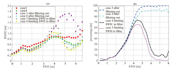
Figure 16.
(a) Ratios and (b) RMSEs of outliers by means of a neural network filter for different SWHs.
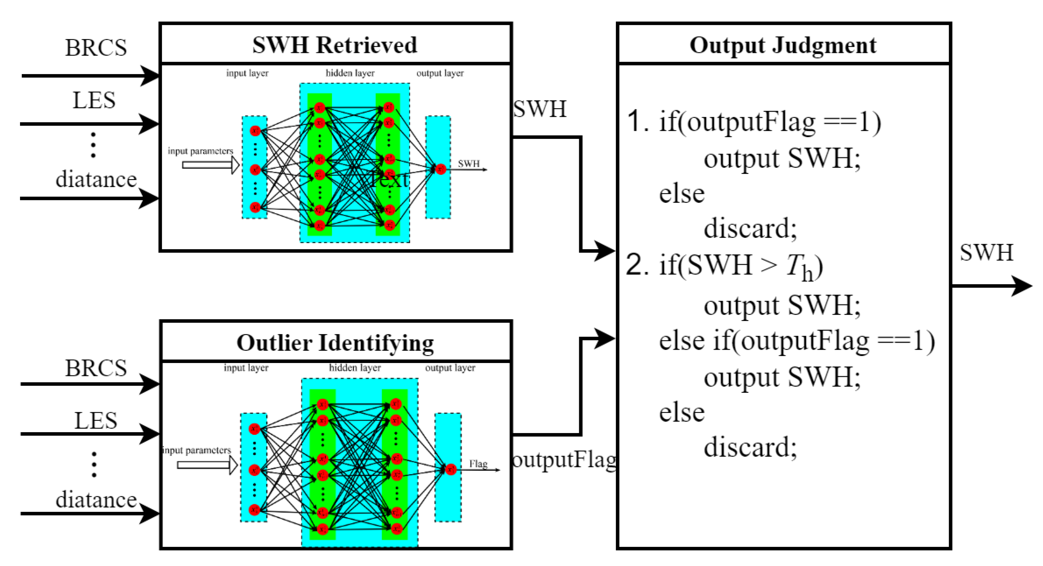
In Figure 17, a combined framework for the SWH retrieval and the outlier identification is depicted. Two neutral networks are used to retrieve SWH and to identify outliers. Once the SWH and the identity are generated, they are used to determine whether the retrieved SWH is credible. The one method is simply to identify whether the retrieved SWH is an outlier. The other method is when the retrieved SWH is below a given threshold, only the SWH identified as good samples is credible.
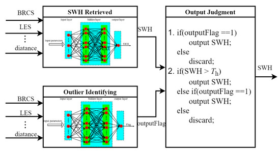
Figure 17.
Combined framework of SWH retrieval and outlier identification.
7. Comparison with Buoy and Jason-3 Data
It is necessary to assess the SWH retrieval performance with an independent SWH measurement. For this purpose, the SWHs from the NDBC buoys and Jason-3 altimters are also collected. A reasonable retrieved SWH performance with respect to the buoy data is found. For the third and fourth case, the RMSEs are 0.57 m and 0.45 m, respectively. Correspondingly, 33.25% and 22.42% of the data are identified as the outliers and filtered out. Compared to the ECMWF verification, the results show worse performance. The reasons are as follows:
- Compared to buoy SWH, the ECMWF data used to train the neural network has a bias and RMSE of 0.09 m and 0.29 m.
- The neural network is trained using the global samples; however, the comparison with buoy SWH is limited in the Gulf of Mexico and Hawaii. In the Gulf of Mexico, the bias and RMSE of the retrieved SWH are larger than those in other regions.
To improve the performance of the neural network retrieving SWH, one feasible remedy is the cross-calibration between the retrieved SWH and buoy SWH, such as adjusting and refining the trained neural network using the match-ups of the CYGNSS measurements and buoy data. This requires a large number of the match-ups. In this study, only 4600 match-ups between the CYGNSS and buoy data are obtained, so they are not sufficient to support this approach.
The retrieved SWH is also in agreement with the SWHs from the Jason-3 Ku-band and C-band altimeters. The RMSEs between the retrieved SWH and Ku-band data are 0.50 m and 0.45 m, respectively, for the third and fourth case. Compared to the C-band data, the third and fourth case have the RMSEs of 0.57 m and 0.53 m, respectively. The discarded outliers account for 11.59% and 10.74% of the total retrieved SWH for the third and fourth case. The C-band SWH has a larger RMS than the Ku-band SWH. i.e., the C-band SWH contains lager error than the Ku-band SWH. This causes a better consistency of the retrieved SWH with the Ku-band SWH than the C-band SWH.
8. Discussion
The SNR of 72.66% of the CYGNSS data were below 5.0 dB. In this SNR interval, the SNR has an important influence on the retrieval performance. For the future spaceborne mission, increasing the system gain of the receiver is desirable to improve the retrieval performance. The GPS PRN and spaceborne ID also impacted the retrieval performance. More advanced calibration approaches should be exploited to weaken the inter-satellite bias. Above 100 GNSS satellites are in orbit, and it is possible for the follow-on missions to synchronously receive and process the signals from several GNSS systems. It was demonstrated that the CYGNSS is capable of receiving the BeiDou B1C and Galileo E1 signal [58,59]. When the number of the visible satellites in the instantaneous field of view is above the processing channel number, a satellite selection have to be performed to choose more proper signals to obtain a better retrieval performance. When the incidence angle was above , the data with a higher incidence angle provided a more precise retrieval; therefore, the signal with a higher incidence angle can be preferentially selected. The GNSS-R measurement is also closely related to the receiver status and platform attitude, such as low noise amplifier (LNA) and analog-digital (A/D) converters in radio frequency (RF) components [60,61]. When these variables are considered as the inputs of the neural networks, the retrieval performances could be further improved.
The developed neural network can be applied to predict the global SWH from 0.25 to 8 m using the CYGNSS data. In total, 89 million data pairs were collected; however, 88.7% of the SWHs are from 1.0 m to 3.0 m, and only 0.01% are larger than 6 m. The performances of the neural networks for the SWH over 6 m were not able to be effectively addressed. The SWHs in marine disaster events, such as typhoons, are usually large. In the future, the investigation of the case studies for marine events will be undertaken.
Seasonal variations in swell and wind-driven waves were found in [50,62]. When the month is used as the input of the neural network, the RMSEs between the retrieved SWH and ECEMF data were respectively reduced to 0.53 m and 0.45 m from 0.59 m 0.49 m for the cases without and with wind speed. This demonstrates that seasonal information is helpful to improve the retrieval performance.
Due to the limitation of the CYGNSS satellite’s inclination, the CYGNSS observation mainly covered the latitude from S to N. The retrieval performances depended on the geographical parameters. The performances did not address the high-latitude region using the CYGNSS data. We hoped that this assessment will be performed for the other spaceborne GNSS-R missions, such as Spire [63], FSSCat [64], and FY-3E [65].
9. Conclusions
In this study, the potential of retrieving SWH using the CYGNSS data was explored. It is difficult to develop an analytical expression of retrieving SWH, therefore, the neural network was used. Two cases were investigated. The input parameters of the one case were the NBRCS, LES, SNR, antenna gain, incidence angle, azimuth angle, latitude, longitude, and the distance from the specular point to the coastline. This case represented the independent retrieval using only the GNSS-R data. The other case also considered wind speed as an input. This case represented the retrieval combining the GNSS-R data and the auxiliary data. The developed neural networks had one input layer, three hidden layers with the hyperbolic tangent as the transfer function and 30 neurons, one output layer with the PELU as the transfer function. For the case without wind speed, the bias and RMSE of −0.13 and 0.59 m were obtained. Once wind speed is considered as the input, the bias and RMSE are −0.09 and 0.49 m, respectively.
Data quality control is a significant approach to improve the retrieval performance. The rigid threshold method can improve the performance; however, it discarded most of the good samples so that the sample number rapidly decreases. To synchronously improve retrieval performance and ensure a high sample number, a soft data filter was designed and developed. The assessment results showed that the RMSEs of the retrieved SWH were reduced to 0.45 m and 0.40 m, and only 16.0% and 14.9% of the samples were removed for the cases without and with wind speed. Unfortunately, this approach introduced an increasing RMSE at high SWH, and filtered out the most of high-SWH samples. To solve this problem, a limited data filter, which only performed the data filter for the retrieved SWH below a given threshold, was proposed. The results showed that the limited data filter retained the most of samples and improved the high-SWH performance.
In the comparison of the retrieved SWH with the buoy data, the RMSEs of 0.57 m and 0.45 for the cases without and with wind speed, respectively, were obtained. Compared to remote sensing, the buoys can provide more precise SWHs. The buoy data can be used to cross-calibrate and refine the trained neural network; however, this task needs a large number of buoy data. The retrieved SWH is also in agreement with the SWHs from the Jason-3 Ku-band and C-band altimeters.
Author Contributions
Methodology, F.W., D.Y. and L.Y.; software, F.W.; validation, F.W.; data curation, F.W.; writing—original draft preparation, F.W.; writing—review and editing, D.Y. and L.Y.; visualization, F.W.; funding acquisition, F.W., D.Y. and L.Y. All authors have read and agreed to the published version of the manuscript.
Funding
This research was funded by the Postdoctoral Innovative Talent Support Program (BX20200039), the Postdoctoral Fund (2021M700319), the National Natural Science Foundation of China (42104031), and the Financial Support for BeiDou Technology Achievement Transformation and Industrialization of Beihang (BARI2003).
Institutional Review Board Statement
Not applicable.
Informed Consent Statement
Not applicable.
Data Availability Statement
Not applicable.
Acknowledgments
We would like to thank the National Aeronautics and Space Administration (NASA) and the European Center for Medium-range Weather Forecasts (ECMWF) for providing the CYGNSS measurement and reanalysis product used in this work.
Conflicts of Interest
The authors declare no conflict of interest.
References
- Steele, K.E.; Teng, V.C.; Wang, D.W.C. Wave direction measurements using pitch-roll buoys. Ocean. Eng. 1992, 19, 349–375. [Google Scholar] [CrossRef]
- Ebuchi, N.; Kawamura, H. Validation of wind speeds and significant wave heights observed by the TOPEX altimeter around Japan. J. Oceanogr. 1994, 50, 479–487. [Google Scholar] [CrossRef]
- Abdalla, S.; Janssen, P.A.E.M.; Biddlot, J.R. Jason-2 OGDR wind and wave products: Monitoring, validation and assimilation. Mar. Geod. 2010, 33, 239–255. [Google Scholar] [CrossRef]
- Jia, Y.; Yang, J.; Lin, M.; Zhang, Y.; Ma, C.; Fan, C. Global assessments of the HY-2B measurements and cross-calibrations with Jason-3. Remote Sens. 2020, 12, 2470. [Google Scholar] [CrossRef]
- Abdalla, S. SARAL/AltiKa wind and wave products: Monitoring, validation and assimilation. Mar. Geod. 2015, 38, 365–380. [Google Scholar] [CrossRef]
- Li, X.M.; Lehner, S.; Bruns, T. Ocean wave integral parameter measurements using Envisat ASAR wave mode data. IEEE Trans. Geosci. Remote Sens. 2011, 49, 155–174. [Google Scholar] [CrossRef] [Green Version]
- Quach, B.; Glaser, Y.; Stopa, J.E.; Mouche, A.A.; Sadowski, P. Deep Learning for Predicting Significant Wave Height From Synthetic Aperture Radar. IEEE Trans. Geosci. Remote Sens. 2021, 3, 1859–1867. [Google Scholar] [CrossRef]
- Wang, H.; Yang, J.; Lin, M.; Li, W.; Zhu, J.; Ren, L.; Cui, L. Quad-polarimetric SAR sea state retrieval algorithm from Chinese Gaofen-3 wave mode imagattes via deep learning. Remote Sens. Environ. 2022, 273, 112969. [Google Scholar] [CrossRef]
- Alpers, W.; Hasselmann, K. Spectral signal to clutter and thermal noise properties of ocean wave imaging synthetic aperture radars. Int. J. Remote Sens. 1982, 3, 423–446. [Google Scholar] [CrossRef]
- Guo, J.; He, Y.; Perrrie, W.; Shen, H.; Chu, X. A new model to estimate significant wave heights with ERS-1/2 scatterometer data. Chin. J. Oceanol. Limnol. 2009, 27, 112–116. [Google Scholar] [CrossRef]
- Guo, J.; He, Y.; Chu, X.; Cui, L.; Liu, G. Wave parameters retrieved from QuickSCAT data. Can. J. Remote Sens. 2009, 35, 345–351. [Google Scholar] [CrossRef]
- Wang, H.; Yang, Y.J.; Zhu, J.; Ren, L.; Liu, Y.; Li, W.; Chen, C. Estimation of significant wave heights from ASCAT scatterometer data via deep learning network. Remote Sens. 2021, 13, 195. [Google Scholar] [CrossRef]
- Wang, J.K.; Aouf, L.; Dalphinet, A.; Zhang, Y.G.; Xu, Y.; Hauser, D.; Liu, J.Q. The wide swath significant wave height: An innovative reconstruction of significant wave heights from CFOSAT’s SWIM and scatterometer using deep learning. Geopjysical Res. Lett. 2021, 48, e2020GL091276. [Google Scholar] [CrossRef]
- Heron, S.F.; Heron, M.L. A comparison of algorithm for extracting significant wave height from HF radar ocean backscatter spectra. J. Atmos. Ocean. Technol. 1998, 15, 1157–1163. [Google Scholar] [CrossRef]
- Foti, G. Spaceborne GNSS reflectometry for ocean winds: First results from the UK TechDemoSat-1 mission. Geophys. Res. Lett. 2006, 42, 5435–5441. [Google Scholar] [CrossRef] [Green Version]
- Pascual, D.; Clarizia, M.P.; Ruf, C.S. Spaceborne Demonstration of GNSS-R scattering cross section sensitivity to wind direction. IEEE Geosci. Remote Sens. Lett. 2021, 19, 1–5. [Google Scholar] [CrossRef]
- Li, W.; Rius, A.; Fabra, F.; Cardellach, E.; Ribo, S.; Martin-Neira, M. Revisiting the GNSS-R Waveform Statistics and Its Impact on Altimetric Retrievals. IEEE Trans. Geosci. Remote Sens. 2018, 56, 2854–2871. [Google Scholar] [CrossRef]
- Zhang, G.; Xu, Z.; Wang, F.; Yang, D.; Xing, J. Evaluation and Correction of Elevation Angle Influence for Coastal GNSS-R Ocean Altimetry. Remote Sens. 2021, 13, 2978. [Google Scholar] [CrossRef]
- Wei, L.; Cardellach, E.; Fabra, F.; Ruis, A.; Martin-Neira, M. First spaceborne phase altimetry over sea ice using TechDemoSat-1 GNSS-R signal. Geophys. Res. Lett. 2017, 44, 8369–8376. [Google Scholar]
- Zhu, Y.; Tao, T.; Zou, J.; Yu, K.; Wickert, J.; Semmling, M. Spaceborne GNSS reflectometry for retrieving sea ice concentration using TDS-1 data. IEEE Geosci. Remote Sens. Lett. 2021, 18, 612–616. [Google Scholar] [CrossRef]
- Lv, J.; Zhang, R.; Tu, J.; Liao, M.; Pang, J.; Yu, B.; Li, K.; Xiang, W.; Fu, Y.; Liu, G. A GNSS-IR Method for Retrieving Soil Moisture Content from Integrated Multi-Satellite Data That Accounts for the Impact of Vegetation Moisture Content. Remote Sens. 2021, 13, 2442. [Google Scholar] [CrossRef]
- Munoz-Martin, J.F.; Llaveria, D.; Herbert, C.; Pablos, M.; Park, H.; Camps, A. Soil Moisture Estimation Synergy Using GNSS-R and L-Band Microwave Radiometry Data from FSSCat/FMPL-2. Remote Sens. 2021, 13, 994. [Google Scholar] [CrossRef]
- Unwin, M.; Jales, P.; Tye, J.; Gommenginger, C.; Foti, G.; Rosello, J. Spaceborne GNSS-reflectometry on TechDeMoSat-1: Early mission operations and exploitation. IEEE J. Sel. Top. Appl. Earth Obs. Remote Sens. 2016, 9, 4525–4539. [Google Scholar] [CrossRef]
- Ruf, C.; Atlas, R.; Chang, P.; Clarizia, M. Zavorotny, V.U. New ocean winds satellite mission to probe hurricanes and tropical convection. Bull. Am. Meteorol. Soc. 2016, 97, 385–395. [Google Scholar] [CrossRef]
- Jing, C.; Niu, X.; Duan, C.; Lu, F.; Di, G.; Yang, X. Sea Surface Wind Speed Retrieval from the First Chinese GNSS-R Mission: Technique and Preliminary Results. Remote Sens. 2019, 11, 3013. [Google Scholar] [CrossRef] [Green Version]
- Soulat, F.; Caparrini, M.; Germain, O.; Lopez-Dekker, P.; Taani, M.; Ruffini, G. Sea state monitoring using coastal GNSS-R. Geophys. Res. Lett. 2004, 31, 133–147. [Google Scholar] [CrossRef] [Green Version]
- Alonso-Arroyo, A.; Camps, A.; Park, H.; Pascual, D.; Onrubia, R.; Martin, F. Retrieval of significant wave height and mean sea surface level using the GNSS-R interference pattern technique: Results from a three-month filed campaign. IEEE Trans. Geosci. Remote Sens. 2015, 53, 3198–3209. [Google Scholar] [CrossRef] [Green Version]
- Martin, F.; Camps, A.; Fabra, F.; Rius, A.; Martin-Neira, M.; D’Addio, S.; Alonso, A. Mitigation of Direct Signal Cross-Talk and Study of the Coherent Component in GNSS-R. IEEE Geosci. Remote. Sens. Lett. 2015, 12, 279–283. [Google Scholar] [CrossRef]
- Clarizia, M.P.; Gommenginger, C.P.; Gleason, S.T.; Srokosz, M.A.; Galdi, C.; Di Bisceglie, M. Analysisi of GNSS-R delay-Doppler maps from the UK-DMC satellite over the ocean. Geophys. Res. Lett. 2009, 36, L02608. [Google Scholar] [CrossRef] [Green Version]
- Soisuvarn, S.; Jelenak, Z.; Said, F.; Chang, P.S.; Egido, A. The GNSS reflectometry response to the ocean surface winds and waves. IEEE J. Sel. Top. Appl. Earth Obs. Remote Sens. 2016, 9, 4678–4699. [Google Scholar] [CrossRef]
- Chen-Zhang, D.D.; Ruf, C.; Ardhuin, F.; Park, J. GNSS-R nonlocal sea state dependencies: Model and empirical verification. J. Geophys. Res. Oceans. 2016, 121, 8379–8394. [Google Scholar] [CrossRef] [Green Version]
- Peng, Q.; Jin, S. Significant wave height estimation from spaceborne Cyclone-GNSS reflectometry. Remote Sens. 2019, 11, 584. [Google Scholar] [CrossRef] [Green Version]
- Haupt, S.E.; Pasini, A.; Marzban, C. Artificial Intelligence Methods in the Environmental Science; Springer: Berlin/Heidelberg, Germany, 2008. [Google Scholar]
- Liu, Y.; Collett, I.; Morton, Y.J. Application of neural network to GNSS-R wind speed retrieval. IEEE Tran. Geosci. Remote Sens. 2019, 57, 9756–9766. [Google Scholar] [CrossRef]
- Reynolds, J.; Clarizia, M.; Santi, E. Wind speed estimation from CYGNSS using artificial neural network. IEEE J. Sel. Top. Appl. Earth Obs. Remote Sens. 2020, 13, 708–716. [Google Scholar] [CrossRef]
- Yan, Q.; Huang, W. Sea ice sensing from GNSS-R data using convolutional neural network. IEEE Geosci. Remote Sens. Lett. 2018, 15, 1510–1514. [Google Scholar] [CrossRef]
- Ruf, C.S.; Chew, C.; Lang, T.; Morris, M.G.; Nave, K.; Ridley, A.; Balasubramaniam, R. A new paradigm in Earth environmental Monitoring with the CYGNSS small satellite constellation. Sci. Rep. 2018, 8, 8782. [Google Scholar] [CrossRef] [PubMed] [Green Version]
- Ruf, C.S.; Gleason, S.; Jelenak, Z.; Katzberg, S.; Ridley, A.; Rose, R.; Scherrer, J.; Zavorotny, V. The CYGNSS nanosatellite constellation hurricane mission. In Proceedings of the 2012 IEEE International Geoscience and Remote Sensing Symposium, Munich, Germany, 22–27 July 2012. [Google Scholar]
- CYGNSS (Cyclone Global Navigation Satellite System). Available online: https://earth.esa.int/web/eoportal/satellite-missions/c-missions/cygnss (accessed on 24 September 2021).
- Gleason, S.; Ruf, C.S.; Clarizia, M.P.; O’Brien, A.J. Calibration and unwrapping of the normalized scattering cross section for the cyclone global navigation satellite system. IEEE Trans. Geosci. Remote Sens. 2016, 54, 2495–2509. [Google Scholar] [CrossRef]
- Clarizia, M.P.; Ruf, C.S.; Jales, P.; Gommenginger, C. Spaceborne GNSS-R minimum variance wind speed estimator. IEEE Trans. Geosci. Remote Sens. 2014, 52, 6829–6843. [Google Scholar]
- Blagus, R.; Lusa, L. Class prediction for high-dimensional class-imbalanced data. BMC Bioinform. 2010, 11, 523. [Google Scholar] [CrossRef] [PubMed] [Green Version]
- Zhai, W.; Zhu, J.; Fan, X.; Yan, L.; Chen, C.; Tian, Z. Preliminary calibration results for Jason-3 and Sentinel-3 altimeters in the Wanshan Islands. J. Oceanol. Limnol. 2021, 39, 458–471. [Google Scholar] [CrossRef]
- Pierson, W.J.; Moskowitz, L.S. A proposed spectral form for sully developed wind seas based on the similarity theory of S.A Kitaigorodskii. J. Geophys. Res. 1964, 69, 386–395. [Google Scholar]
- Voronovich, A.G.; Zavorotny, V.U. Theoretical model for scattering of radar signals in Ku and C bands from a rough sea surface with breaking waves. Waves Rand. Media 2001, 11, 247–269. [Google Scholar] [CrossRef]
- Brown, G. Backscattering from a Gaussian distributed perfectly conducting rough surface. IEEE Trans. Antennas Propag. 1978, 26, 472–482. [Google Scholar] [CrossRef] [Green Version]
- Clarizia, M.P.; Ruf, C.S. Wind speed retrieval algorithm for the cyclone global navigation satellite system (CYGNSS) mission. IEEE Trans. Geosci. Remote Sens. 2016, 54, 4419–4432. [Google Scholar] [CrossRef]
- Asgarimehr, M.; Zhelavskaya, I.; Foti, G.; Reich, S.; Wichert, J. A GNSS-R geophysical model function: Machine learning for wind speed retrievals. IEEE Geosci. Remote Sens. Lett. 2020, 17, 1333–1337. [Google Scholar] [CrossRef]
- Chen, G.; Chapron, B.; Ezraty, R.; Vandemark, D. A global view of swell and wind sea climate in the ocean by satellite altimeter and scatteometer. J. Atmos. Ocean. Technol. 2002, 19, 1849–1859. [Google Scholar] [CrossRef]
- Hanley, K.E.; Belchen, S.E.; Sullivan, P.P. A global climatology of wind-wave interaction. J. Phys. Oceanogr. 2010, 40, 1263–1282. [Google Scholar] [CrossRef] [Green Version]
- Li, X.; Yang, D.; Yang, J.; Zheng, G.; Han, G.; Nan, Y.; Li, W. Analysis of coastal wind speed retrieval from CYGNSS mission using artificial neural network. Remote Sens. Environ. 2021, 260, 112454. [Google Scholar] [CrossRef]
- Kalra, R.; Dec, M.C. Derivation of coastal wind and wave parameters from offshore measurements of TOPEX satellite using ANN. Coast. Eng. 2007, 54, 187–196. [Google Scholar] [CrossRef]
- Ulaby, F.T.; Moore, R.K.; Fung, A.K. Microwave Remote Sensing: Active and Passive—Volume II: Radar Remote Sensing and Surface Scattering and Emission Theory, 3rd ed.; Artech House: Norwood, MA, USA, 1982. [Google Scholar]
- Steigenberger, P.; Thoelert, S.; Montenbruck, O. GNSS satellite transmit power and its impact on orbit determination. J. Geod. 2018, 92, 609–624. [Google Scholar] [CrossRef]
- Balasubramaniam, R.; Ruf, C. Neural Network Based Quality Control of CYGNSS Wind Retrieval. Remote Sens. 2020, 12, 2859. [Google Scholar] [CrossRef]
- Guo, W.; Du, H.; Cheong, J.W.; Southwell, B.; Dempster, A.G. GNSS-R wind speed retrieval of sea surface based on particle swarm optimization algorithm. IEEE Trans. Geosci. Remote Sens. 2022, 60, 1–14. [Google Scholar] [CrossRef]
- Said, F.; Jelenak, Z.; Chang, P.S.; Soisuvarn, S. An Assessment of CYGNSS Normalized Bistatic Radar Cross Section Calibration. IEEE J. Sel. Top. Appl. Earth Obs. Remote Sens. 2019, 12, 50–65. [Google Scholar] [CrossRef]
- Li, W.; Cardellach, E.; Ribo, S.; Rius, A.; Zhou, B. First spaceborne demonstrationof BeiDou-3 signals for GNSS reflectometry from CYGNSS constellation. Chin. J. Aeronaut. 2021, 34, 1–10. [Google Scholar] [CrossRef]
- Li, W.; Cardellach, E.; Ribo, S.; Oliveras, S.; Rius, A. Exploration of Multi-Mission Spaceborne GNSS-R Raw IF Data Sets: Processing, Data Products and Potential Applications. Remote Sens. 2022, 14, 1344. [Google Scholar] [CrossRef]
- Chu, X.; He, J.; Song, H.; Qi, Y.; Sun, Y.; Bai, W.; Li, W.; Wu, Q. Multimodal deep learning for heterogeneous GNSS-R data fusion and ocean wind speed retrieval. IEEE J. Sel. Top. Appl. Earth Observ. Remote Sens. 2020, 13, 5971–5981. [Google Scholar] [CrossRef]
- Hammond, M.L.; Fotiu, G.; Gommenginger, C.; Srokosz, M. Temporal variability of GNSS-Reflectometry ocean wind speed retrieval performance during the UK TechDemoSat-1 mission. Remote Sens. Environ. 2020, 242, 111744. [Google Scholar] [CrossRef]
- Young, I.R. Seasonal variability of the global ocean wind and wave climate. Int. J. Climatol. 1999, 19, 931–950. [Google Scholar] [CrossRef]
- Nguyen, V.A.; Nogues-Correig, O.; Yuasa, T.; Masters, D.; Irisov, V. Initial GNSS phase altimetry measurements from the spire satellite constellation. Geophys. Res. Lett. 2020, 47, e2020GL088308. [Google Scholar] [CrossRef]
- Herbert, C.; Munoz-Martin, J.F.; Llaveria, D.; Pablos, M.; Camps, A. Sea Ice Thickness Estimation Based on Regression Neural Networks Using L-Band Microwave Radiometry Data from the FSSCat Mission. Remote Sens. 2021, 13, 1366. [Google Scholar] [CrossRef]
- Sun, Y.; Liu, C.; Du, Q.; Wang, X.; Bai, W.; Kirchengast, G.; Xia, J.; Meng, X.; Wang, D.; Cail, Y.; et al. Global navigation satellite system occultation sounder II (GNOS II). In Proceedings of the 2017 IEEE International Geoscience and Remote Sensing Symposium (IGARSS), Fort Worth, TX, USA, 23–28 July 2017; pp. 1189–1192. [Google Scholar]


Publisher’s Note: MDPI stays neutral with regard to jurisdictional claims in published maps and institutional affiliations. |
© 2022 by the authors. Licensee MDPI, Basel, Switzerland. This article is an open access article distributed under the terms and conditions of the Creative Commons Attribution (CC BY) license (https://creativecommons.org/licenses/by/4.0/).