Article

Toward Atmospheric Correction Algorithms for Sentinel-3/OLCI Images of Productive Waters

1
Laboratory of Hydrology and Ecology of Inland Waters, Radiophysical Department, Lobachevsky State University of Nizhny Novgorod, 23 Gagarin Avenue, 603022 Nizhny Novgorod, Russia
2
Institute of Applied Physics of the Russian Academy of Sciences, 46 Ulyanov St., 603950 Nizhny Novgorod, Russia
3
Marine Hydrophysical Institute of the Russian Academy of Sciences, 2 Kapitanskaya St., 299011 Sevastopol, Russia
4
P.P. Shirshov Institute of Oceanology, 36 Nakhimovsky Prospekt, 117997 Moscow, Russia
*
Author to whom correspondence should be addressed.
Remote Sens. 2022, 14(15), 3663; https://doi.org/10.3390/rs14153663
Submission received: 31 May 2022 / Revised: 7 July 2022 / Accepted: 28 July 2022 / Published: 30 July 2022
(This article belongs to the Special Issue Remote Sensing of Land Water Bodies)

Abstract

:
Atmospheric correction of remote sensing imagery over optically complex waters is still a challenging task. Even algorithms showing a good accuracy for moderate and extremely turbid waters need to be tested when being used for eutrophic inland basins. Such a test was carried out in this study on the example of a Sentinel-3/OLCI image of the productive waters of the Gorky Reservoir during the period of intense blue-green algal bloom using data on the concentration of chlorophyll a and remote sensing reflectance measured from the motorboat at many points of the reservoir. The accuracy of four common atmospheric correction (AC) algorithms was examined. All of them showed unsatisfactory accuracy due to incorrect determination of atmospheric aerosol parameters and aerosol radiance. The calculated aerosol optical depth (AOD) spectra varied widely (AOD(865) = 0.005 − 0.692) even over a small area (up to 10 × 10 km) and correlated with the measured chlorophyll a. As a result, a part of the high water-leaving signal caused by phytoplankton bloom was taken as an atmosphere signal. A significant overestimation of atmospheric aerosol parameters, as a consequence, led to a strong underestimation of the remote sensing reflectance and low accuracy of the considered AC algorithms. To solve this problem, an algorithm with a fixed AOD was proposed. The fixed AOD spectrum was determined in the area with relatively “clean” water as 5 percentiles of AOD in all water pixels. The proposed algorithm made it possible to obtain the remote sensing reflectance with high accuracy. The slopes of linear regression are close to 1 and the intercepts tend to zero in almost all spectral bands. The determination coefficients are more than 0.9; the bias, mean absolute percentage error, and root-mean-square error are notably lower than for other AC algorithms.

1. Introduction

Many national programs, such as the Global Environment Monitoring System for Freshwater, USGS Water Resources Mission Area, Water Framework Directive, etc., are devoted to optical remote sensing of water quality in inland waters. In this regard, much attention is paid to the development of national and regional observation systems that provide reliable information on water quality, its variability, as well as the impact of human activity on it. The development of such systems, even for small freshwater basins, became possible with the launch of a constellation of Sentinel-3 A/B satellites equipped with OLCI (Ocean and Land Color Instrument) radiometers of medium (300 m) resolution, performing measurements in 21 spectral channels suitable for monitoring optically complex waters, with a frequency of 1 time per day [1].
According to OLCI operational products [2], OLCI water-leaving reflectance for open-water products mainly meets S3 mission requirements. It shows average relative percentage differences within the range of 5–10% in comparison with in situ measurements and other satellite missions. However, the approved accuracy assessment of complex-water products has not yet been published.
In this regard, research aimed at studying the accuracy of atmospheric correction (AC) of OLCI imagery for estimating the concentrations of Chl a, TSM, and CDOM in optically complex waters is of high value. Recently, many papers have been devoted to these issues [3,4,5,6,7,8,9,10,11,12,13].
The accuracy of different AC algorithms for processing Sentinel-3/OLCI images is evaluated in [14,15,16,17] to find the best one for specific basin conditions. Unfortunately, these results often turn out to be contradictory, and the best algorithm, in some cases, shows low accuracy for others. This once again underlines the difficulty of atmospheric correction in optically complex waters and the need to take into account the regional characteristics of reservoirs to obtain satisfactory estimates of the concentrations of the optical components of water.
Validation of five atmospheric correction algorithms for estimation of ocean color retrievals over optically complex coastal waters of France was performed in [15]. The authors of this study came to the conclusion about the high accuracy of the C2RCC [18,19] and POLYMER [20] algorithms, which outperformed the BAC/ACC (ESA’s standard AC algorithm for OLCI ocean processing) [21,22] and NASA [23,24] algorithms. The authors of [17], who evaluated the AC accuracy for turbid waters in the coastal zone of Belgium, came to the opposite conclusion: the BAC algorithm was one of the best; C2RCC and POLYMER algorithms showed the worst accuracy, especially in the bands of 665 and 709 nm, which are important for chlorophyll a and turbidity retrievals in Case II waters.
In [16], the accuracy of four AC algorithms was estimated, and Chl a-retrieval algorithms were evaluated for small highly productive freshwater basins in South Africa. The authors also noted the impossibility of using AC algorithms based on neural networks to recover the concentration of Chl a because the neural networks distort the shape of the remote sensing reflectance ( R r s ) spectrum in the red and NIR bands. In contrast to the coastal waters studied in [15,17], where the AC algorithms generally showed plausible results, the accuracy of AC algorithms for small highly productive water basins was not high enough [16]. Despite this, the authors emphasized that it is still possible to obtain reasonable estimates of the concentration of Chl a using models based on the fluorescent line height (FLH) and the maximum chlorophyll index (MCI) if the retrieved R r s spectra preserve their real shape. According to [16], highly productive freshwater basins differ significantly in their characteristics from pure ocean waters and coastal zones of the seas. In order to obtain reliable satellite products for them, several issues related to both atmospheric correction (including more complex atmospheric aerosol properties characteristic of rural areas and the impact of the adjacency effects) and radiometric measurement and water sampling methods (accounting for horizontal and vertical inhomogeneity due to bloom patchiness and vertical distribution of cyanobacteria) need to be solved.
New methods of atmospheric correction for Sentinel-3/OLCI images were proposed in [14,17]. The Dark Spectrum Fitting (DSF) atmospheric correction algorithm was described in [17]. The AC algorithm over extremely turbid waters, using the SWIR band potential at 1016 nm, was described in [14]. The presence of a high (non-physical) correlation between water and aerosol signals in the bands of 865 and 1016 nm for BAC and NASA algorithms, respectively, was also noted in [14]. Overestimation level-2 OLCI aerosol products have also been noted in [25], which can significantly affect the accuracy of the determination of aerosol type during atmospheric correction.
In this study, the AC accuracy of Sentinel-3/OLCI images for the Gorky Reservoir, under conditions of intense cyanobacteria bloom, is studied. We have limited ourselves to considering some of the common AC algorithms available in the l2gen processor (SeaDAS), as well as radiometric level-2 products (OL_2_WFR—OLCI level-2 water full resolution) provided by EUMETSAT. We also proposed an atmospheric correction with a fixed aerosol optical depth (AOD), which was determined in an image fragment with relatively clean water, where the water-leaving reflectance can be considered negligible (Section 2.3.2 and Section 3.2).
The in situ measurements were carried out from a gliding motorboat, which made it possible to obtain more than 2900 radiometric spectra in about 1.5 h. When comparing these measurements with the resolution of the OLCI image, 5 to 77 spectra fell into one image pixel (Section 3.1.1), depending on the motorboat direction and velocity. By averaging multiple in situ measurements within a single pixel, we hope to obtain more relevant data for the validation of satellite images under conditions of significant spatial inhomogeneity of the optical properties of water caused by cyanobacteria bloom patchiness. A large number of measurements on the motorboat route, similar by form to “8”, ensure the repeated passage of the same areas after a certain time interval and enable one to estimate the spatial and temporal variability of the water reflectance within one pixel of the satellite image (Section 3.1.1 and Section 3.1.2).
This paper continues the study of AC algorithm validation and the regional bio-optical algorithm development for the Gorky Reservoir: one of the important water basins of the Russian Federation, characterized by high spatiotemporal variability of the water’s optical properties. Previous results for Sentinel-2/MSI imagery were published in [26].

2. Materials and Methods
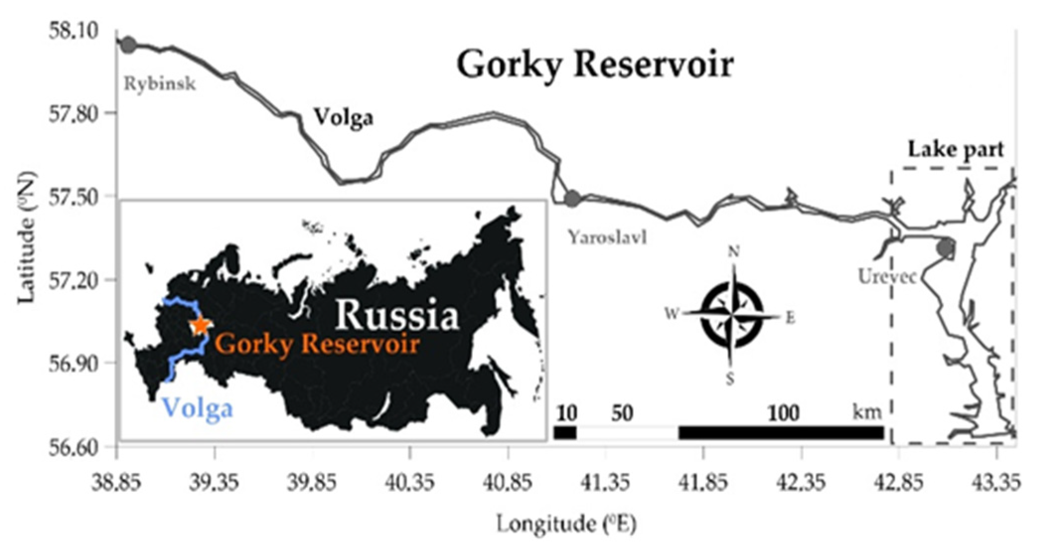
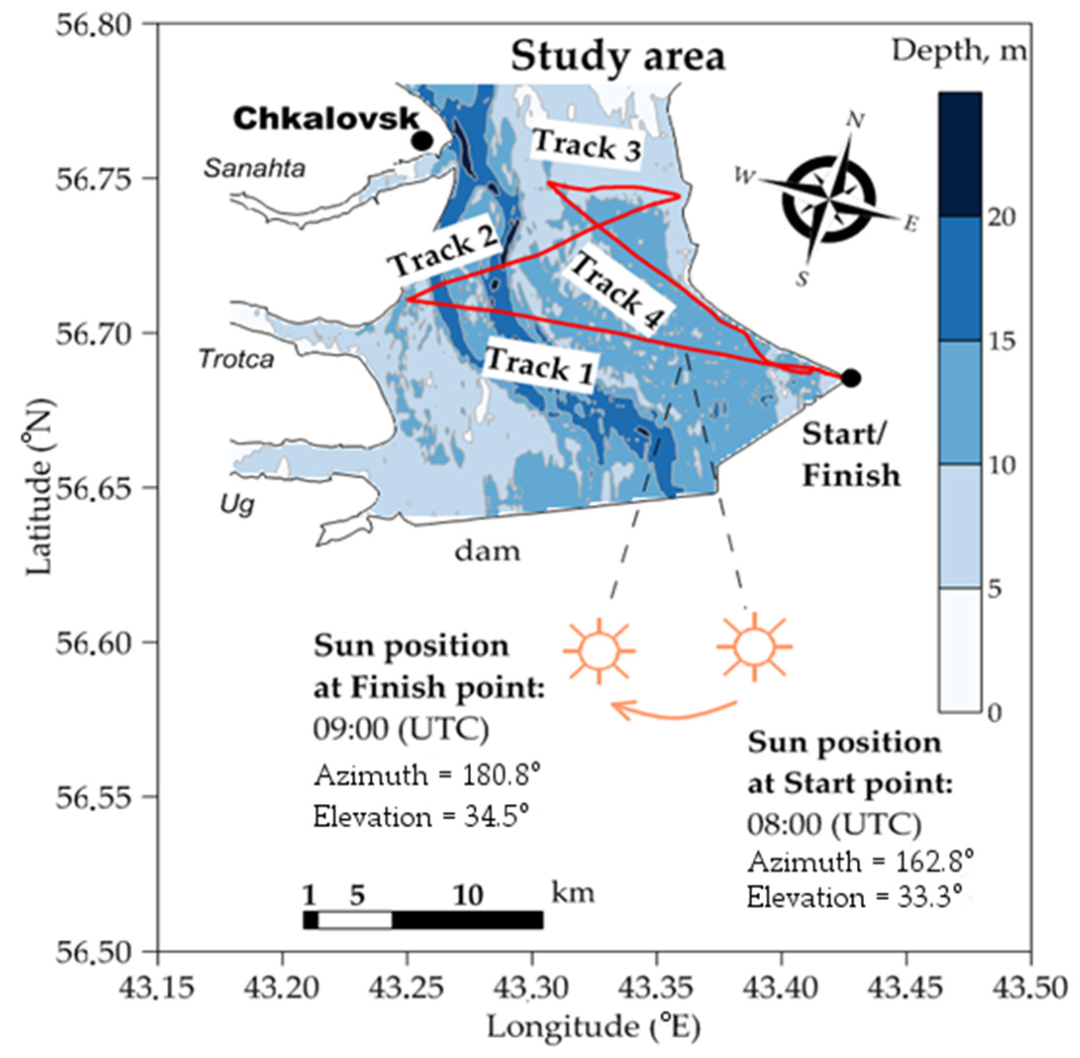
2.1. Study Area

The Gorky Reservoir (56.65°–58.08°N, 38.83°–43.37°E), located on the Volga River, has a length of 427 km and covers an area of 1590 km2 (Figure 1). The last 100 km form the lake part. The average and maximum depths of the lake part are 3.65 m and 26.6 m, respectively. The trophic status of the reservoir is eutrophic; however, it changes to hypertrophic at the end of summer due to intense blue-green algal bloom. According to our measurements conducted in 2015–2019, the concentrations of main water constituents in the reservoir were in the range of 0.5–460 mg/m3 for Chl a, 9–21 mg/L for total organic carbon (TOC), and 5–20 mg/L for TSM. The Secchi depth varied from 0.2 to 3.5 m, and the euphotic zone, from 1.0 to 4.1 m. The water surface temperature reached 32 degrees.
Water discharge through the dam has a significant effect on the current velocity in the reservoir [27]. The average current velocity along the Volga channel is about 3–6 cm/s at the usual discharge of 1000 m3/s, and it increases up to 10–15 cm/s in places where the reservoir narrows. At a discharge of 1300 m3/s, the current velocity reaches 25 cm/s in front of the dam. The mentioned water discharges are typical of summer, but they can increase several times after intense rains, which significantly changes the structure of the current in the reservoir. Non-stationary currents and non-uniform winds lead to the formation of complex patterns of phytoplankton and suspended matter over the reservoir, including a vortex structure and frontal zones with the highest water constituent concentration (Figure 2). Their dimensions vary from tens of meters to several kilometers.

2.2. Field Measurements

2.2.1. Radiometric Measurements

In situ measurements were carried out on 22 September 2018 under the Sentinel-3 overpass at 8:06 UTC. The sky was clear, the weather was sunny, and the water surface was calm. Blue-green algae concentrated near the surface and looked similar to inhomogeneous spatial structures of random shapes, often with sharp boundaries (similar to ones in Figure 2b–e) moving at different velocities, affected by the current.
To minimize the above-mentioned features, we used the technique of high-speed non-station-based measurements, which we have already tested earlier [26]. This method is based on simultaneous remote sensing reflectance and measurements of Chl a from a high-speed gliding motorboat with allowance for the NASA recommendations on the geometry of observation relative to the position of the Sun [28]. According to Figure 3, the latter varied in the range of 162.8°–180.8° and 33.3°–34.5° for azimuth angle and solar elevation, respectively, during 1 h of in situ measurements. Simultaneously, the motorboat had a route consisting of 4 straight tracks with a total length of about 30 km. Each track was about 6–8 km and took 10–15 min; meanwhile, the position of the Sun changed in azimuth and elevation by 4.5° and 0.3°, respectively. Thus, we considered that the lighting conditions had not changed (but we controlled it; see below). This statement was important, since in the absence of three spectrometers for above-water measuring of the directional upwelling radiance L u , the sky radiance L r reflected by the water surface, and the downwelling irradiance E d , we used only one spectrometer: an Ocean Optics USB2000+ with a field of view (FOV) of 20°, a spectral range of 400–750 nm, a spectral resolution of 1 nm, and a frequency of 1 Hz for sequential measurements of listed characteristics. In particular, the above-water directional upwelling radiance was registered continuously along each track at a cruise velocity of 8 m/s, providing the spatial resolution of the data equivalent to 8 m. Two other characteristics were measured before the beginning and at the end of each track, each for 1 min.
For continuous measurements, the spectrometer was fixed at a zenith angle of 30° on the bow railing as the most forward point of the motorboat and oriented in the direction of movement (Figure 4). For fine-tuned azimuth correction at each track, the spectrometer could be turned mechanically to the desired angle. We used this opportunity when changing the track to maintain a 90-degree angle between the spectrometer orientation and the direction of the Sun, as it is allowed by the NASA protocol [28]. In fact, the azimuthal position of the Sun, the observation geometry, and the reservoir elongation seriously limited the choice of possible motorboat directions. As a result, we chose the route already mentioned above and presented in Figure 3. The proposed route made it possible to cross the reservoir several times and cover a large water area, encountering bloom spots of different intensities.
The obtained time series of L u , L r , and E d were smoothed by the median filter. After that, L r and E d were averaged over 1 min. The irradiance values obtained every 10–15 min (at the beginning and at the end of each track) served as an indicator of lighting stability. As a result, the remote sensing reflectance R r s was calculated similarly to Mobley [29]:
R r s = L u L ¯ r E ¯ d
where L ¯ r and E ¯ d are the time-averaged values of L r and E d . In the presence of three synchronized spectrometers, the instantaneous values of R r s can be calculated using Equation (1) but using the instantaneous values of the three characteristics included in it.

2.2.2. LiDAR Measurements

Simultaneously with radiometric measurements, we used pre-calibrated ultraviolet fluorescence LiDAR UFL-9 for continuous measurement of the concentration of Chl a. Fluorescence LiDAR systems are widely used around the world for registering bio-optical parameters of the oceans, seas, and inland waters [30,31,32]. Various studies have been conducted on the comparison of LiDAR measurements and satellite data of MODIS, MERIS, and SeaWiFS radiometers in the open sea [33,34,35,36,37]. LiDAR systems are especially relevant for small inland basins, where the spatial characteristics of water quality parameters change very fast. The mentioned LiDAR UFL-9 has been involved in in situ measurements all over the world, e.g., in the Atlantic Ocean, in the Black, the Kara, the Aral, the Caspian, the Baltic, the South China, the Barents, the North, and the Mediterranean Seas, on Lakes Balaton and Issyk-Kul, and in the Ikshinsky and Gorky Reservoirs.
The high quality of LiDAR data is achieved due to LiDAR’s physical principles and technical characteristics. The UV fluorescent LiDAR UFL-9 analyzes returned signal from the dual-excitation Nd:YAG laser pulses (355 and 532 nm) emitted at a frequency of 2 Hz with an energy of 2 mJ. Detection is carried out sequentially in 11 bands (355, 385, 404, 424, 440, 460, 499, 532, 620, 651, and 685 nm) at stations with simultaneous water sampling for the instrument calibration, and across four bands (355, 404, 440, and 685 nm) simultaneously in transect mode while the motorboat is moving. The fluorescence intensities at 440 nm (CDOM) and 685 nm (Chl a) and backscattering signal at 355 nm (TSM) are normalized to the Raman scattering at 404 nm and then calibrated using a set of laboratory-measured concentrations of CDOM, Chl a, and TSM.
Being tested on a great number of water basins, LiDAR allows the measurement of bio-optical properties with high accuracy for non-contact and express methods. According to [38,39], the total relative measurement error of UFL-9 is 10% for TSM and CDOM and 16% for Chl a. LiDAR’s signal processing and calibration are exhaustively described in [40].
It is important to note that the LiDAR calibration is carried out for each water basin independently and ideally for each expedition. For this purpose, water samples are taken from a large water area to cover the widest possible range of variability in the optical properties of water and transferred to the laboratory to restore concentrations of the main water constituents. This can be done on the eve of the day of satellite acquisition or after the satellite overpass. In addition, it is not necessary to wait for calibration results, since LiDAR measures the fluorescence signal in relative units. Thus, these signals can be converted into absolute units at any time by comparing the fluorescence signals at the time of water sampling at the stations with the obtained concentrations of optically active components. In our case, a good correlation between fluorescence signal at 685 nm and Chl a concentration was established:
Chl   a = 0.019 x 685 3.109 ,   R 2 = 0.91 ,
where x 685 is the LiDAR signal at 685 nm (Chl a fluorescence) in Raman units and R 2 is the determination coefficient [26].
Returning to the measurement technique at the Gorky Reservoir, LiDAR UFL-9 with a FOV of 1° was also installed onto the bow railing, slightly behind the spectrometer (Figure 4). It was oriented at an angle of 30° and 45° to the zenith and motion direction, respectively. Such an arrangement of LiDAR and spectrometer was necessary for conducting passive optical observations and active laser sensing of the unperturbed water surface in front of the motorboat and minimizing splashes and sun glints on the FOV.
The temporal resolution of the used LiDAR was 2 Hz, which ensures data collection with a spatial resolution of 4 m at a cruise velocity of 8 m/s. As a result, we obtained around 7200 measurements of Chl a for 1.5 h over a water area of about 50 sq. km.

2.2.3. Water Sampling

To recalculate fluorescence LiDAR signals into the concentration of Chl a, surface water samples were collected from a depth of 0–30 cm using clear polyethylene bottles at 10 stations. The samples were delivered to the shore within 1–2 h in a refrigerator at a temperature of −4 °C. Filtration was carried out using 47 mm Whatman GF/F fiberglass filters with a pore size of 0.7 μm with a low vacuum (~0.2 bar). The filtered volume was 2 L. The filters were frozen at −16 °C and stored in dark conditions for 1 week. In the laboratory, the concentration of Chl a was determined using the spectrophotometric method [41] and calculated according to the equation for mixed phytoplankton [42]. Chl a was extracted into 10 mL of 90% aqua acetone solution twice an hour. The extracts were clarified twice by centrifugation for 10 min at a velocity of 8000 r/min. The concentration of Chl a was measured by an SF-14 spectrophotometer (Russia) and pre-calibrated using pure chlorophyll (Sigma) as a standard. Despite the fact that the spectrophotometric method does not satisfy the NASA protocols [43], it is often used to retrieve the concentration of Chl a, as it is the most accessible method providing reliable accuracy (e.g., [44,45,46]). Intercomparison of the spectrophotometric method with two other methods, valid according to NASA protocols, namely, fluorometric and high-performance liquid chromatography methods, was performed, e.g., in [47,48].

2.3. Sentinel-3/OLCI Imagery and Image Processing

2.3.1. Match-Ups for Satellite Validation and Spatial–Temporal Variability within a Pixel

The RGB image (the surface reflectance in the bands of 665, 560, and 490 nm) of the Gorky Reservoir on 22 September 2018 is presented in Figure 5a. The red line marks the motorboat route.
During the expedition, we obtained more than 2900 radiometric spectra in about 1 h. All of them were averaged within the Sentinel-3/OLCI pixel image. Depending on the direction and velocity of the motorboat, there are 5 to 77 R r s spectra per pixel of the image. In contrast to the common approach [49], OLCI-retrieved R r s were not derived from a 5 × 5 pixel block centered above the location of the in situ measurement for the validation procedure. Due to the significant spatial inhomogeneity of the optical properties of water, this approach considerably increases the difference between in situ and area-averaged satellite measurements, which, in turn, worsens the validation results [17]. Therefore, for validation, OLCI R r s was taken only from those pixels where the in situ radiometric measurements fell on. The concentration of Chl a according to LiDAR measurements was averaged in the same way. After averaging, 127 coinciding pairs of satellite and in situ measurements were obtained and used to validate the AC algorithm.
Multiple measurements within one satellite pixel enabled one to estimate the spatial variability of the optical properties of water under cyanobacteria bloom conditions. For this purpose, several pixels along the motorboat route with different color intensities proportional to the algal concentration (Figure 5c) were selected, and the variation coefficient of R r s was calculated over the entire spectral range (see Section 3.1.1).
Moreover, the motorboat route consisted of 4 intersecting tracks (Figure 5d). This made it possible to perform measurements in the same area after a certain time interval and, therefore, to estimate the temporal variability of the optical properties of water in the Gorky Reservoir. The motorboat tracks #2 and #4 intersected in pixel #1*. The beginning of track #1 and the end of track #4 intersected in pixels #2*–5*. Thus, 5 pixels were selected and pixel-averaged R r s spectra for the different times were analyzed in them.

2.3.2. Atmospheric Correction

We used a cloud-free Sentinel-3A/OLCI image of the Gorky Reservoir on 22 September 2018 (Figure 5a). The OLCI level-1 (L1B) imagery was processed by the SeaWIFS Data Analysis System software (SeaDAS) v7.5.3 (https://seadas.gsfc.nasa.gov (accessed on 29 June 2022)).
Atmospheric correction (AC) of remote sensing imagery over optically complex waters is still challenging. Even algorithms showing a good accuracy for moderate and extremely turbid waters [50,51,52] need to be tested when being used for eutrophic inland basins. The water-leaving reflectance in the NIR bands is not negligible there. In the case of exceptional algal bloom, one can observe a surface manifestation of various algae forms (floating algae, mats, scum, etc.) even in SWIR bands. This, in turn, makes it difficult to determine the parameters of atmospheric aerosol and aerosol radiance, which eventually affects the accuracy of retrieving the remote sensing reflectance. To determine the AC algorithm which is most suitable for the conditions of the Gorky Reservoir, we performed validation of some common algorithms included in SeaDAS (l2gen processor). Particular attention was paid to validation of the OLCI level-2 water full resolution (OL_2_WFR) obtained according to a processing baseline v.2.23 [2] and provided by EUMETSAT. We also studied the suitability of atmospheric correction with a fixed aerosol, the parameters of which can be determined using a fragment of the image with relatively clean water, where the water-leaving reflectance can be considered negligible, or using in situ measurements of the aerosol optical depth (AOD). The following algorithms were used:
  • The common NASA approach applied to MODIS imagery [23], in which aerosol reflectance is calculated from two NIR bands (779 nm and 865 nm), and then extrapolated to visible bands, together with an iterative procedure for calculating the water-leaving reflectance in the NIR bands [24] (termed ac(779, 865) hereafter). Standard flagging was used, namely, pixels with WATER flag, excluding ATM_FAIL, HIGLINT, HILT, HIPOL, HISATZEN, HISOLZEN, SEAICE, CLDICE, and STRAYTLIGHT;
  • The algorithm is similar to the previous one, but the NIR–SWIR bands of 865 nm and 1012 nm are used to calculate the aerosol reflectance (hereinafter referred to as ac(865, 1012)). Due to the strong water absorption in SWIR, these bands are successfully used in atmospheric correction over turbid waters [52,53]. We are exploring the possibility of using an OLCI SWIR band at 1016 nm to improve AC over eutrophic waters. Masking is the same as in 1;
  • The MUMM algorithm (hereinafter referred to as MUMM) is a well-known algorithm for estimating the water-leaving reflectance in turbid waters, based on the assumption of spatial homogeneity of NIR band relations for aerosol and water-leaving reflectance in the subscene [50]. In fact, MUMM is an algorithm with a fixed type of aerosol, the concentration of which can vary in an image. MUMM often shows a significant improvement in turbid coastal waters than the ac(779, 865) algorithm. Masking is the same as in 1;
  • OL_2_WFR radiometric products (hereinafter referred to as L2W) contain the water-leaving reflectance ρw, on 16 spectral bands, related to the remote sensing reflectance Rrs by the relation Rrs = ρw/π. They are obtained in accordance with the ESA’s standard atmospheric correction procedure combining two approaches: (i) a baseline AC, which is a combination of the black-water approach with the bright pixel atmospheric correction [21,22], and (ii) an alternative AC, in which atmospheric parameters and water-leaving reflectance are inverted using neural networks [54]. The following set of common quality flags was used: pixels including INLAND_WATER, excluding AC_FAIL and INVALID, CLOUD, CLOUD_AMBIGUOUS, CLOUD_MARGIN, SNOW_ICE, COSMETIC, SATURATED, SUSPECT, HISOLZEN, HIGHGLINT, ADJAC, and WHITECAP. RWNEG* flags were not used, since the presence and number of negative values of remote sensing reflectance were criteria for the suitability of AC algorithm for the Gorky Reservoir;
  • Atmospheric correction using a fixed aerosol, the properties of which are determined by the AOD spectrum (hereinafter referred to as fixed AOD). This method consists of two consecutive calculations using the ac(779, 865) algorithm. Based on the first calculation, the AOD spectra were determined for all water pixels of the area of interest. As our research has shown, the AOD spectra vary widely (AOD(865) = 0.005, …, 0.692) even over a small area (up to 10 × 10 km). Smaller AOD values are found in areas with cleaner water, and larger ones, in waters with a high phytoplankton concentration. Such a large AOD scatter is most likely due not to spatial changes in atmospheric aerosol, but to incorrect determination of aerosol parameters in areas with a high phytoplankton content. To determine the AOD spectra over clean water, which is less susceptible to atmospheric correction errors, we used the fifth percentile of AOD in all water pixels in the study area. Assuming that the properties of the atmospheric aerosol within the study area were constant or varied only slightly, these fixed AOD spectra were further used in the second calculation using l2gen (aer_opt = −8). Approaches in which the aerosol type is determined from the nearest non-turbid area were also implemented in [55,56]. In contrast to these approaches, we assume that both the aerosol type and its optical properties can be considered constant on small spatial scales.
Since SeaDAS (l2gen) is mainly configured for Case I waters; the threshold reflectance for distinguishing water from clouds is very low for eutrophic waters. As a result, waters with intense algal bloom are also masked as clouds and excluded from further calculations. Therefore, in our study, the default threshold reflectance ρ c l o u d ( 865 ) = 0.027 was changed to ρ c l o u d ( 1012 ) = 0.035 . This value was determined empirically according to the condition that reservoir waters where in situ measurements were performed were not masked as clouds. To avoid errors when interpreting objects with high radiance in the NIR bands, this approach is applicable only for cloudless images.
In addition to changing ρ c l o u d , the maximum number of iterations in the procedure for determining the water reflectance in the NIR bands was increased from 10 to 40. A further increase in the maximum number of iterations did not affect the R r s retrieval.
L1B and OL_2_WFR imagery were downloaded from the Copernicus Online Data Access system (CODA) (https://coda.eumetsat.int (accessed on 29 June 2022)).

2.3.3. Accuracy Metrics

The accuracy of the AC algorithm was estimated based on six statistical values, namely, the slope and intercept of linear regression between in situ radiometry and OLCI R r s estimates, the coefficient of determination R2 (which is equal to the square of Spearman’s correlation coefficient), bias, mean absolute percent error (MAPE), and the root-mean-square error (RMSE). The bias, MAPE, and RMSE were calculated as follows:
bias = 1 N i = 1 N ( y i e s t y i o b s ) ,
MAPE = 1 N i = 1 N | y i e s t y i o b s | y i o b s 100 ,
RMSE = 1 N i = 1 N ( y i e s t y i o b s ) 2 ,
where y i e s t and y i o b s are the OLCI-estimated and in situ-measured R r s , respectively, and N is the number of match-ups.

3. Results

3.1. In Situ Measurements

3.1.1. Variations of R r s Spectra within One Pixel

According to LiDAR measurements, the concentration of Chl a varied in the range from 4 to 460 mg/m3 per day of the expedition, and the average, median, and standard deviation of concentration were 57.5, 38.8, and 52.5 mg/m3, respectively. The bright green color in Figure 5a shows a high concentration of algae and water-leaving reflectance near the left bank of the reservoir. Such a wide range of variations was registered due to the repeated crossing of the reservoir from coast to coast.
Figure 5b presents the corresponding measured water-leaving reflectance spectra. All of them are typical of water with high phytoplankton biomass. The troughs at 620 nm and 675 nm related to the absorption of phycocyanin (cyanobacteria pigments) and chlorophyll, respectively, are clearly exhibited in the reflectance. A peak of about 709 nm caused by strong backscattering of algae and absorption by chlorophyll at 675 nm and the water is also distinguished.
Due to spatial inhomogeneity of the optical properties of water caused by the cyanobacteria bloom patchiness, a notable variation in R r s within one pixel of the satellite image takes place (Figure 6). The variability of the concentration of Chl a within a pixel and the pixel-averaged concentration of Chl a is given in Table 1.
It should be noted that spectra shapes within a single pixel are generally the same, but R r s differ greatly, especially in the B6(560), B11(709), and B12(754) bands (pixels #30–60, 110–120). R r s values in pixels of intense green color (pixels #10, 30, 40, 110, and 120) according to the average concentrations of Chl a of 40–130 mg/m3 are an order of magnitude higher than R r s values in dark blue pixels (pixels #20, 50, and 60–100) with concentrations of Chl a of 25–30 mg/m3. The spectra with extremely high R r s in B11(709) and B12(754) bands can be seen in pixels #30, 40, 110, and especially 120. Such spectra usually correspond to surface formations of algae such as mats and surface scum. In pixels #80, 90, and 100, which are distant from the algae accumulation area, the spectra shapes differ significantly. The concentration of Chl a is also high here (16–30 mg/m3), as evidenced by the small R r s in the blue bands and the small troughs at 675 nm. However, algae biomass here obviously is much lower, so the peak at 709 nm is not formed on the R r s spectrum. It should also be noted (Table 1) that the concentration of Chl a can vary by 2–3 times, and sometimes by 4 times within a single pixel (pixels #30 and 120).
The variation coefficients (CV) for R r s in the Sentinel-3 spectral bands are given in Table 2 and the arrangement of pixels is presented in Figure 5c. It is possible to detect some dependence of the variation coefficient on the concentration of Chl a. For example, the variation coefficients for R r s (709) are 5–10% for concentrations of Chl a in the range of 15–25 mg/m3 (pixels #80, 90, and 100). At concentrations of Chl a exceeding 50 mg/m3 (Figure 5c and Table 1), the variation coefficient increases up to 35% (pixels #30, 40, and 110). The highest variation coefficient for R r s (709) has been observed in pixel #120, with an average concentration of Chl a of 104 mg/m3, and is equal to 61%.
Validation of satellite products for Case I water is performed under the assumption of spatial homogeneity of the optical properties of water. The SeaBASS validation system excludes those satellite measurements in which the median CV of calculated R r s in the range of 405–570 nm exceeds 15% [49,57]. Optically complex waters (Case II water), on the contrary, are characterized by high spatial inhomogeneity. Under such conditions, on the one hand, within a block of 5 × 5 pixels (1.5 × 1.5 km for Sentinel-3/OLCI), optical properties can vary by 1–2 orders of magnitude. Therefore, the validation of satellite products in the pixel closest to in situ measurements turns out to be more reasonable.
On the other hand, satellite measurements are pixel-averaged. As can be seen from Figure 6 and Table 2, the CV of R r s within one pixel can vary from 3 to 115% in various spectral bands. At the same time, with an increase in the concentration of Chl a, CV also increases. Thus, comparing pixel-averaged satellite data with measurements conventionally carried out at one station can lead to unreliable results.
In this regard, multiple measurements within one satellite pixel performed on a moving motorboat, under conditions of spatial inhomogeneity of the optical properties of water, seem more preferable, reliable, and statistically justified.

3.1.2. Variations of R r s Spectra in Point with Time

Table 3 presents the averaged concentration of Chl a and the time delay between measurements in pixels (Figure 5c). Pixel-averaged R r s spectra are given in Figure 7, where the blue and red curves correspond to measurements carried out on the forward and reverse motorboat tracks. The number of in situ measurements within one pixel, which is used to obtain the averaged spectrum, is shown in Table 3, and varied from 30 to 77 depending on the position and orientation of the motorboat track relative to the pixel.
Measurements in pixel #1* were repeated after 25 min (Table 3). As a result, we registered an increase in the concentration of Chl a (by about 50%) and R r s (Figure 7). Measurements in the following four pixels (#2*–5*) were performed with a time delay of 74–80 min. In this case, we see an opposite situation with a decrease in the averaged concentration of Chl a by 18–41% and R r s (Figure 7), in general. However, there is one exception in pixel #4*. Here, a slight increase in the average concentration of Chl a was registered due to an increase to 91.3 mg/m3 in the maximum concentration at several measurement points within the pixel.
Comparing R r s spectra in Figure 7, we can state that their temporal variability is significant (20–30% on average) and differs significantly for various regions of the reservoir. Thus, variations are observed in the Volga channel with the highest current velocity after 25 min (pixel #1*) and in a low-flow floodplain (pixels #2*–5*) after 80 min. We consider the obtained results as indicative and aimed at ensuring that other researchers of inland waters do not neglect spatiotemporal variability of the bio-optical properties of water (or prove that there is no such variability for their water bodies). To date, there is a very small number of papers (see, e.g., [58]) in which the issue under consideration would be given sufficient attention.

3.2. Validation of the Remote Sensing Reflectance

The results of R r s validation from OL_2_WFR are shown in Figure 8 with a blue line. The slope of linear dependence (Figure 8a) is negative in all bands except B11(709) and B12(754). The determination coefficient in all bands does not exceed 0.2 (Figure 8b); other accuracy criteria are also low, especially in the blue bands.
Negative R r s spectra are mainly related to the overestimation of aerosol radiance. The distribution of AOD(865) from OL_2_WFR (blue line) and the measured concentration of Chl a (red line) along the motorboat route are shown in Figure 9a. It is obvious that AOD(865) largely repeats the main features of the distribution of the concentration of Chl a. Thus, we can assume that when determining the atmospheric parameters, a significant part of the water-leaving reflectance in the NIR bands was taken into account. As a result, the contribution of the atmosphere was overestimated and, therefore, the retrieved R r s spectra in B1-B10 bands are negative.
The distribution of the concentration of Chl a calculated using a neural network (blue line) (Chl_NN) and measured (red line) along the motorboat route is shown in Figure 9b. The spatial distribution of Chl_NN contradicts the distribution of pixel brightness (algae concentration) in Figure 5a. In the area with intense green color, the concentration of Chl_NN is less than in the area with black color. We can also observe this due to the distribution of Chl a along the motorboat route (Figure 9b). Chl_NN is approximately 0.5 mg/m3, where the measured concentration of Chl a exceeded 100 mg/m3. Conversely, Chl_NN increased to about 8 mg/m3, where measured concentrations are less than 50 mg/m3. Perhaps the reason for the implausible results is that the neural network has not been trained for cases of cyanobacteria bloom [59].
The distribution of the measured and retrieved R r s in B10(681) and B11(709) bands along the motorboat route is shown in Figure 10a,b. One can notice that, in pixels with a high concentration of Chl a (of about 50 mg/m3) (green line), retrieved R r s spectra (blue line) are almost a mirror image of measured R r s spectra (red line), i.e., the peaks of measured R r s spectra at high Chl a correspond to negative peaks of retrieved R r s spectra (pixels #15, 27, 30, and 75). In pixels where Chl a exceeds 100 mg/m3 (pixels #7–13, 117–125), the discontinuities in which R r s spectra are not calculated and equal to NaN are observed. This is also typical of the B1–B10 bands, in which the slope of linear regression is also negative (Figure 8a).
The retrieved R r s spectra repeat the features of R r s spectra measured along the motorboat route in B11(709) and B12(754) bands fairly well, where slopes are positive (Figure 10b). Although the number of negative R r s spectra is small, retrieved R r s differs from the measured R r s by about 2 times where Chl a exceeds 50 mg/m3. R r s is equal to NaN, where Chl a exceeds 100 mg/m3. A scatter plot of measured and retrieved R r s spectra in B10(681) and B11(709) bands is given in Figure 10c,d.
Figure 8, Figure 11 and Figure 12 present the validation results of the restored R r s using other AC algorithms. The accuracy parameters of the MUMM algorithm are plotted with an orange line, ac(779, 865) and ac(865, 1012), with purple and green lines, respectively. Unfortunately, none of the algorithms allowed us to obtain satisfactory results. As for the L2W data, the slopes of linear regression (Figure 8a) are negative in all bands except B11(709) and B12(754), but the determination coefficients are much higher. For ac(779, 865) and ac(865, 1012) algorithms, R2 is 0.45–0.55 in the B4(490), B5(510), and B7-B10 bands, but it is significantly less than for L2W in the B11 and B12 bands (approximately 0.15). The MUMM algorithm made it possible to slightly reduce the amplitude of negative R r s spectra, which reduced the bias and RMSE, but the determination coefficient is 30–50% lower than that for ac(779, 865) and ac(865, 1012), but greater than that for L2W in most bands.
For these three algorithms, AOD and aerosol radiance L a profiles repeat the Chl a distribution along the motorboat route (Figure 11), which reveals an incorrect assessment of water-leaving reflectance in the NIR bands. The R r s distributions retrieved by these AC algorithms are shown in Figure 12. In general, the results are similar to those obtained using the L2W algorithm (Figure 10). R r s is negative or cannot be calculated at all (line breaks) where Chl a exceeds 50 mg/m3. This is a reason for the negative slopes of the linear regression and low-accuracy criteria. R r s spectra obtained due to the ac(865, 1012) and MUMM algorithms have slightly higher values compared to ac(779, 865). However, this increment is not large enough to obtain positive R r s in areas with a high concentration of Chl a. On the contrary, this increment increases the discrepancy with the measurements in pixels with Chl a less than 50 mg/m3 (pixels #50–72 and 75–105).
AOD spectra over clean water, defined as the fifth percentile of AOD in all water pixels by ac(779, 865), were used as inputs for the fixed AOD algorithm. Figure 8 shows that among the algorithms considered, the fixed AOD algorithm (black dotted line) enabled one to retrieve R r s with the highest accuracy. The slopes are close to 1, and the intercepts tend to zero in nearly all bands. The determination coefficients exceed 0.9. Bias, MAPE, and RMSE are notably lower than for other AC algorithms. The B1(400), B2(412), B11(709), and B12(754) bands are an exception, where bias, MAPE, and RMSE increase sharply.
The distribution of retrieved R r s using the fixed AOD algorithm is shown in Figure 13. In contrast to results in Figure 10 and Figure 12, the retrieved R r s spectra repeat the distribution of measured R r s spectra and correspond to the variability of Chl a along the motorboat route. Generally, the retrieved R r s spectra are close to the measured ones, but in pixels with an extremely high concentration of Chl a, R r s spectra may differ by 20–50%.
Spectra of R r s and AOD in some pixels along the motorboat route are shown in Figure 14; pixel arrangement and numbering are presented in Figure 5c. Measured R r s spectra are plotted in red and R r s spectra retrieved using the MUMM algorithm are marked with orange lines; ac(779, 865) and ac(865, 1012) correspond to purple and green lines, respectively, and the fixed AOD is a dotted black line. The AOD spectra (purple line) were calculated on AOD(865) and the Angstrom exponent A(865) using the relation AOT ( λ ) = AOT ( 865 ) ( 865 / λ ) A . The AOD spectrum used in the fixed AOD algorithm was determined by the method described above and was constant in all pixels. The remaining AOD spectra were obtained during the corresponding atmospheric corrections.
The fixed AOD algorithm accurately retrieves R r s spectra in a wide Chl a range of 16–135 mg/m3 (black dotted line), with the exception of B1(400) and B12(412) bands, where retrieved R r s is larger than the measured one, probably due to the adjacency effect. AOD obtained in different AC algorithms for the same pixels (color lines) vary in a wide range. The closer the pixels are to the fixed AOD spectrum, the more accurate retrieved R r s spectra are. AOD spectra shapes obtained using the ac(779, 865) algorithm are similar to the spectra obtained by the L2W algorithm, and the ac(865, 1012) algorithm is similar to MUMM, which can indicate the applicability of these algorithms for different types of waters.

4. Discussion

The accuracy of atmospheric correction of remote sensing imaginary over highly productive waters is affected by the accuracy of the estimation of the water-leaving reflectance in the NIR bands. Unfortunately, none of the considered atmospheric correction algorithms could satisfactorily manage this. The water-leaving reflectance in the NIR bands was underestimated and its part was taken as the aerosol radiance. Calculated AOD and aerosol radiance (Figure 9 and Figure 11) repeated the distribution of the concentration of Chl a along the motorboat route. As a result, a large number of negative R r s spectra were received in pixels with a high concentration of Chl a (Figure 10 and Figure 12). The use of the SWIR band for atmospheric correction (ac(865, 1012) algorithm) and the MUMM algorithm, which operate well in turbid sediment-dominated waters and enable one to nearly get rid of negative R r s , did not solve this problem. These algorithms (especially MUMM) slightly reduced the magnitude of negative R r s spectra, which affected the reduction of negative bias (Figure 8). However, MUMM accuracy was generally worse (the determination coefficient is almost 2 times less in most bands) than the accuracy of the standard NASA ac(779, 865) algorithm. This happened due to the overestimation of R r s in pixels where the concentration of Chl a is less than 50 mg/m3.
It can be seen that all algorithms retrieved R r s well in a certain range of concentrations of Chl a, but beyond it, accuracy significantly deteriorates (Figure 14 and Table 1). The ac(779, 865) algorithm (purple line) operates well when the concentration of Chl a is less than 30 mg/m3 (see pixels #50, 60, 80, 90, and 100). While the concentration of Chl a increases up to 35 mg/m3 (pixels #20 and 70), the accuracy decreases. The ac(865, 1012) (green line) and MUMM (orange line) algorithms overestimate R r s for Chl a below 30 mg/m3 (see pixels #50, 60, and 80), but give slightly better estimates than ac(779, 865) for Chl a in the range of 30–65 mg/m3 (pixels #20, 40, and 70).
CHL_NN product from OL_2_WFR for hyper-eutrophic waters of the Gorky Reservoir does not correctly reproduce either spatial features of the algae distribution or quantitative estimates of their concentration. In comparison with in situ measurements, CHL_NN is inverse, i.e., CHL_NN is low in pixels with a high content of algae, and vice versa. Instead, TSM_NN from OL_2_WFR are high in these pixels, i.e., the algorithm considers that the waters have a high content of mineral suspended matter. Perhaps this is due to the fact that neural network training was not performed for cases of cyanobacteria bloom.
The use of the fixed AOD algorithm showed the highest accuracy of R r s retrieval. Despite the fact that the assumption of the constancy of the optical properties of the aerosol is quite rough, the possible sources of the associated uncertainties were small compared to the errors in determining the aerosol properties and the water-leaving reflectance in the NIR bands according to the standard image-based method. A positive experience of using the 6SV model of atmospheric correction for Sentinel-3/OLCI and Sentinel-2/MSI imagery was described in [16,60]. AOD determined by in situ measurement was considered constant over inland water in their studies. It is possible that for reservoirs with a high algae biomass, the pixel-by-pixel determination of aerosol parameters from satellite imagery is extremely difficult or impossible in principle. Thus, different approaches are required for such cases.
The method for determining the AOD spectrum from the adjacent area of less turbid water has shown a high potential for R r s retrieval. High accuracy was obtained in almost all VIS bands for various R r s spectra shapes (Figure 14), corresponding to a Chl a concentration range of 12–307 mg/m3, on a spatial scale of approximately 10 × 10 km. Further research can be aimed at comparing the image-defined fixed AOD spectrum with in situ measurements and at studying the accuracy variability of the fixed AOD algorithm on larger spatial scales. In addition, to assess the propriety of aerosol model selection for atmospheric correction, we intend to measure AOD using a portable solar photometer MICROTOPS.

5. Conclusions

The accuracy of atmospheric correction of satellite imaginary over highly productive waters is affected by the accuracy of estimating the water-leaving reflectance in near-infrared bands. Using the example of the highly productive Gorky Reservoir and an extensive data set of in situ measurements, our research has shown that the common atmospheric correction algorithms, demonstrating good accuracy for moderate and extremely turbid waters, significantly overestimate the atmosphere contribution to productive inland waters. In particular, none of the considered atmospheric correction algorithms (NASA, ESA, and MUMM) could satisfactorily manage this. The water-leaving reflectance in near-infrared bands was underestimated, and its significant part was mistaken for aerosol radiance, which led to an incorrect estimation of the aerosol optical depth. We have clearly demonstrated that the aerosol optical depth and aerosol radiance profiles repeat the chlorophyll a distribution over the reservoir, which reveals an incorrect estimation of water-leaving reflectance in the NIR bands. The proposed fixed aerosol optical depth algorithm, in which aerosol optical depth spectrum was determined from the adjacent area of less turbid water, made it possible to accurately to retrieve Rrs spectra with a determination coefficient close to 1 in almost all spectral bands in waters with chlorophyll variations in the range of 12–307 mg/m3. The obtained result complements the results for Sentinel-2 imagery published in our previous paper.
Validation of satellite measurements for highly productive inland reservoirs cannot be reduced only to the search for an optimal AC algorithm. Radiometric measurement and water sampling methods should be corrected with allowance for the horizontal and vertical inhomogeneity caused by cyanobacteria bloom. The coefficient of variation of R r s within one pixel varied from 3 to 115% in various spectral bands in the Gorky Reservoir. Thus, a comparison of pixel-averaged satellite data with measurements at a single station could lead to unreliable results. Temporal variability of R r s is also significant in the Gorky Reservoir and it was, on average, 20–30% in 20–80 min. To minimize the impact of time variability, the time window for validation points should be no more than one hour.

Author Contributions

A.M. implemented the methodology and in situ measurements and wrote the manuscript. S.F. performed data processing, analyses, validation, and wrote the manuscript. V.P. performed LiDAR measurements and data processing and wrote the manuscript. All authors have read and agreed to the published version of the manuscript.

Funding

This research was funded by the Federal Academic Leadership Program “Priority-2030” and by the Russian Foundation for Basic Research regarding the organization and conduct of LiDAR measurements (Project No. 20-55-75002) and regarding the LiDAR data processing (Project No. 19-55-80004).

Acknowledgments

We are grateful to Dmitriy Kostitsyn for using his unique high-speed motorboat in our in situ measurements, Boris Konovalov for laboratory analysis, and George Leshov for his assistance in equipment setup. The authors also thank the anonymous reviewers for their useful comments and suggestions.

Conflicts of Interest

The authors declare no conflict of interest.

References

  1. Donlon, C.; Berruti, B.; Buongiorno, A.; Ferreira, M.H.H.; Féménias, P.; Frerick, J.; Goryl, P.; Klein, U.; Laur, H.; Mavrocordatos, C.; et al. The Global Monitoring for Environment and Security (GMES) Sentinel-3 mission. Remote Sens. Environ. 2012, 120, 37–57. [Google Scholar] [CrossRef]
  2. Sentinel-3A Product Notice—OLCI Level-2 Ocean Colour. Operational Products and Full-Mission Reprocessed Time Series. EUM/OPS-SEN3/DOC/17/964713 S3A.PN.OLCI-L2M.02. Is. 11/01/2018. Ver.1.0. Available online: https://www-cdn.eumetsat.int/files/2020-04/pdf_s3a_pn_olci_l2_rep.pdf (accessed on 30 May 2022).
  3. Blix, K.; Li, J.; Massicotte, P.; Matsuoka, A. Developing a New Machine-Learning Algorithm for Estimating Chlorophyll-a Concentration in Optical Complex Waters: A Case Study for High Northern Latitude Waters by Using Sentinel 3 OLCI. Remote Sens. 2019, 11, 2076. [Google Scholar] [CrossRef] [Green Version]
  4. Riddick, C.A.; Hunter, P.D.; Domínguez Gómez, J.A.; Martinez-Vicente, V.; Présing, M.; Horváth, H.; Kovács, A.W.; Vörös, L.; Zsigmond, E.; Tyler, A.N. Optimal Cyanobacterial Pigment Retrieval from Ocean Colour Sensors in a Highly Turbid, Optical Complex Lake. Remote Sens. 2019, 11, 1613. [Google Scholar] [CrossRef] [Green Version]
  5. Xue, K.; Ma, R.; Wang, D.; Shen, M. Optical Classification of the Remote Sensing Reflectance and Its Application in Deriving the Specific Phytoplankton Absorption in Optical Complex Lakes. Remote Sens. 2019, 11, 184. [Google Scholar] [CrossRef] [Green Version]
  6. Watanabe, F.; Alcântara, E.; Imai, N.; Rodrigues, T.; Bernardo, N. Estimation of Chlorophyll-a Concentration from Optimizing a Semi-Analytical Algorithm in Productive Inland Waters. Remote Sens. 2018, 10, 227. [Google Scholar] [CrossRef] [Green Version]
  7. Toming, K.; Kutser, T.; Uiboupin, R.; Arikas, A.; Vahter, K.; Paavel, B. Mapping Water Quality Parameters with Sentinel-3 Ocean and Land Colour Instrument imagery in the Baltic Sea. Remote Sens. 2017, 9, 1070. [Google Scholar] [CrossRef] [Green Version]
  8. Lins, R.C.; Martinez, J.-M.; Motta Marques, D.D.; Cirilo, J.A.; Fragoso, C.R. Assessment of Chlorophyll-a Remote Sensing Algorithms in a Productive Tropical Estuarine-Lagoon System. Remote Sens. 2017, 9, 516. [Google Scholar] [CrossRef] [Green Version]
  9. Eleveld, M.A.; Ruescas, A.B.; Hommersom, A.; Moore, T.S.; Peters, S.W.M.; Brockmann, C. An Optical Classification Tool for Global Lake Waters. Remote Sens. 2017, 9, 420. [Google Scholar] [CrossRef] [Green Version]
  10. Wolanin, A.; Soppa, M.A.; Bracher, A. Investigation of Spectral Band Requirements for Improving Retrievals of Phytoplankton Functional Types. Remote Sens. 2016, 8, 871. [Google Scholar] [CrossRef] [Green Version]
  11. Lin, J.; Lyu, H.; Miao, S.; Pan, Y.; Wu, Z.; Li, Y.; Wang, Q. A two-step approach to mapping particulate organic carbon (POC) in inland water using OLCI images. Ecol. Indic. 2018, 90, 502–512. [Google Scholar] [CrossRef]
  12. Blix, K.; Pálffy, K.; Tóth, V.R.; Eltoft, T. Remote Sensing of Water Quality Parameters over Lake Balaton by Using Sentinel-3 OLCI. Water 2018, 10, 1428. [Google Scholar] [CrossRef] [Green Version]
  13. Pahlevan, N.; Smith, B.; Schalles, J.; Binding, C.; Cao, Z.; Ma, R.; Alikas, K.; Kangro, K.; Gurlin, D.; Nguyễn Hà, N.; et al. Seamless retrievals of chlorophyll- a from Sentinel-2 (MSI) and Sentinel-3 (OLCI) in inland and coastal waters: A machine-learning approach. Remote Sens. Environ. 2020, 240, 111604. [Google Scholar] [CrossRef]
  14. Gossn, J.I.; Ruddick, K.G.; Dogliotti, A.I. Atmospheric Correction of OLCI Imagery over Extremely Turbid Waters Based on the Red, NIR and 1016 nm Bands and a New Baseline Residual Technique. Remote Sens. 2019, 11, 220. [Google Scholar] [CrossRef] [Green Version]
  15. Mograne, M.A.; Jamet, C.; Loisel, H.; Vantrepotte, V.; Mériaux, X.; Cauvin, A. Evaluation of Five Atmospheric Correction Algorithms over French Optical-Complex Waters for the Sentinel-3A OLCI Ocean Color Sensor. Remote Sens. 2019, 11, 668. [Google Scholar] [CrossRef] [Green Version]
  16. Kravitz, J.; Matthews, M.; Bernard, S.; Griffith, D. Application of Sentinel 3 OLCI for chl-a retrieval over small inland water targets: Successes and challenges. Remote Sens. Environ. 2020, 237, 111562. [Google Scholar] [CrossRef]
  17. Vanhellemont, Q.; Ruddick, K. Atmospheric correction of Sentinel-3/OLCI data for mapping of suspended particulate matter and chlorophyll-a concentration in Belgian turbid coastal waters. Remote Sens. Environ. 2021, 256, 112284. [Google Scholar] [CrossRef]
  18. Doerffer, R.; Schiller, H. MERIS Regional Coastal and Lake Case 2 Water Project Atmospheric Correction ATBD, Rep. GKSS-KOF-MERIS-ATBD01; GKSS Research Center, Institute of Coastal Research: Geesthacht, Germany, 2008; Volume 1. [Google Scholar]
  19. Brockmann, C.; Doerffer, R.; Peters, M.; Stelzer, K.; Embacher, S.; Ruescas, A. Evolution of the C2RCC neural network for Sentinel 2 and 3 for the retrieval of ocean color products in normal and extreme optically complex waters. In Proceedings of the Living Planet Symposium 2016, Prague, Czech Republic, 9–13 May 2016; European Space Agency Special Publication: Prague, Czech Republic, 2016; Volume ESA SP-740, pp. 1–6. [Google Scholar]
  20. Steinmetz, F.; Deschamps, P.Y.; Ramon, D. Atmospheric correction in presence of sun glint: Application to MERIS. Opt. Express 2011, 19, 9783–9800. [Google Scholar] [CrossRef] [Green Version]
  21. Antoine, D.; Morel, A. A multiple scattering algorithm for atmospheric correction of remotely sensed ocean color (MERIS instrument): Principle and implementation for atmospheres carrying various aerosols including absorbing ones. Int. J. Remote Sens. 1999, 20, 1875–1916. [Google Scholar] [CrossRef]
  22. Moore, G.F.; Aiken, J.; Lavender, S.J. The atmospheric correction of water color and the quantitative retrieval of suspended particulate matter in Case II waters: Application to MERIS. Int. J. Remote Sens. 1999, 20, 1713–1733. [Google Scholar] [CrossRef]
  23. Gordon, H.R.; Wang, M. Retrieval of water-leaving radiance and aerosol optical thickness over the oceans with SeaWiFS: A preliminary algorithm. Appl. Opt. 1994, 33, 443–452. [Google Scholar] [CrossRef]
  24. Bailey, S.W.; Franz, B.A.; Werdell, P.J. Estimation of near-infrared water-leaving reflectance for satellite ocean color data processing. Opt. Express 2010, 18, 7521–7527. [Google Scholar] [CrossRef]
  25. Zibordi, G.; Mélin, F.; Berthon, J.-F. A Regional Assessment of OLCI Data Products. IEEE Geosci. Remote Sens. Lett. 2018, 15, 1490–1494. [Google Scholar] [CrossRef]
  26. Molkov, A.A.; Fedorov, S.V.; Pelevin, V.V.; Korchemkina, E.N. Regional Models for High-Resolution Retrieval of Chlorophyll a and TSM Concentrations in the Gorky Reservoir by Sentinel-2 Imagery. Remote Sens. 2019, 11, 1215. [Google Scholar] [CrossRef] [Green Version]
  27. Kapustin, I.A.; Molkov, A.A. Structure of Currents and Depth in the Lake Part of the Gorky Reservoir. Russ. Meteorol. Hydrol. 2019, 7, 110–117. [Google Scholar]
  28. Mueller, J.L.; Pietras, C.; Hooker, S.B.; Austin, R.W.; Miller, M.; Knobelspiesse, K.D.; Frouin, R.; Holben, B.; Voss, K. Ocean Optics Protocols for Satellite Ocean Color Sensor Validation, Revision 4, Volume II: Instrument Specifications, Characterization and Calibration (NASA/TM-2003-21621/Rev-Vol II); Goddard Space Flight Space Center: Greenbelt, MD, USA, 2003; pp. 1–56. [Google Scholar]
  29. Mobley, C.D. Estimation of the remote sensing reflectance from above–water methods. Appl. Optics 1999, 38, 7442–7455. [Google Scholar] [CrossRef]
  30. Hyper-Spectral Laser Induced Fluorescent Lidar Sensors Systems OceanVisual. Available online: www.oceanvisuals.no (accessed on 29 May 2022).
  31. Raymetrics Fluorescent Lidar. Available online: https://raymetrics.com/fluorescence-lidar/ (accessed on 29 May 2022).
  32. LDI Fluorescent Lidars. Available online: www.ldi-innovation.com/index.php/hyperspectral-lif-lidar (accessed on 29 May 2022).
  33. Fiorani, L.; Okladnikov, I.G.; Palucci, A. Remote Sensing of the Southern Ocean by MERIS, MODIS, Seawifs and ENEA Lidar. J. Optoelectron. Adv. Mater. 2008, 10, 1482–1488. [Google Scholar]
  34. Hoge, F.E.; Lyon, P.E.; Swift, R.N.; Yungel, J.K.; Abbott, M.R.; Letelier, R.M.; Esaias, W.E. Validation of Terra-MODIS Phytoplankton Chlorophyll Fluorescence Line Height. I. Initial Airborne Lidar Results. Appl. Opt. 2003, 42, 2767–2771. [Google Scholar] [CrossRef] [PubMed]
  35. Ma, S.; Liu, Z.S.; Zhang, K.L.; Li, Z.G.; He, S.Y. Field Experiment of an Airborne Oceanographic Lidar and Comparison with a Moderate Resolution Imaging Spectroradiometer. Lasers Eng. 2006, 16, 413–421. [Google Scholar]
  36. Moreno-Madrinan, M.J.; Al-Hamdan, M.Z.; Rickman, D.L.; Muller-Karger, F.E. Using the Surface Reflectance MODIS Terra Product to Estimate Turbidity in Tampa Bay, Florida. Remote Sens. 2010, 2, 2713–2728. [Google Scholar] [CrossRef]
  37. Palmer, S.C.J.; Kutser, T.; Hunter, P.D. Remote Sensing of Inland Waters: Challenges, Progress and Future Directions. Remote Sens. Environ. 2015, 157, 1–8. [Google Scholar] [CrossRef] [Green Version]
  38. Palmer, S.C.; Pelevin, V.V.; Goncharenko, I.V.; Kovács, A.; Zlinszky, A.; Présing, M.; Horváth, H.; Nicolás-Perea, V.; Balzter, H.; Tóth, V. Ultraviolet Fluorescence Lidar (UFL) as a Measurement Tool for Water Quality Parameters in Turbid Lake Conditions. Remote Sens. 2013, 5, 4405–4422. [Google Scholar] [CrossRef]
  39. Pelevin, V.; Zlinszky, A.; Khimchenko, E.; Toth, V. Ground truth data on Chlorophyll-a, chromophoric dissolved organic constituents and suspended sediment concentrations in the upper water layer as obtained by LIF Lidar at high spatial resolution. Int. J. Remote Sens. 2017, 38, 1967–1982. [Google Scholar] [CrossRef] [Green Version]
  40. Pelevin, V.; Zavialov, P.; Konovalov, B.; Zlinszky, A.; Palmer, S.; Toth, V.; Goncharenko, I.; Khymchenko, L.; Osokina, V. Measurements with high spatial resolution of Chlorophyll-a, CDOM and total suspended constituents in coastal zones and inland water basins by the portable UFL Lidar. In Proceedings of the 35th EARSeL Symposium—European Remote Sensing: Progress, Challenges and Opportunities, Stockholm, Sweden, 15–18 June 2015. [Google Scholar]
  41. SCOR-UNESCO. Report of SCOR-UNESCO Working Group 17 on Determination of Photosynthetic Pigments in SEA WATER. In Monograph of Oceanography Methodology; UNESCO: Paris, France, 1966; Volume 1, pp. 9–18. [Google Scholar]
  42. Jeffrey, S.W.; Humphrey, G.F. New spectrophotometric equations for determining chlorophylls a, b, c1 and c2 in higher plants, algae and natural phytoplankton. Biochem. Physiol. Pflanz. 1975, 167, 191–194. [Google Scholar] [CrossRef]
  43. Mueller, J.L.; Bidigare, R.R.; Trees, C.; Balch, W.M.; Dore, J.; Drapeau, D.T.; Karl, D.; Van Heukelem, L.; Perl, J. Ocean Optics Protocols for Satellite Ocean Color Sensor Validation, Revision 5, Volume 5: Biogeochemical and Bio-Optical Measurements and Data Analysis Protocols; Goddard Space Flight Space Center: Greenbelt, MD, USA, 2003; pp. 5–24. [Google Scholar]
  44. Bao, Y.; Tian, Q.; Chen, M.A. Weighted Algorithm Based on Normalized Mutual Information for Estimating the Chlorophyll-a Concentration in Inland Waters Using Geostationary Ocean Color Imager (GOCI) Data. Remote Sens. 2015, 7, 11731–11752. [Google Scholar] [CrossRef] [Green Version]
  45. Alikas, K.; Kangro, K.; Reinart, A. Detecting cyanobacterial blooms in large North European lakes using the Maximum Chlorophyll Index. Oceanologia 2010, 52, 237–257. [Google Scholar] [CrossRef] [Green Version]
  46. Moses, W.J.; Gitelson, A.A.; Berdnikov, S.; Povazhnyy, V. Satellite estimation of Chlorophyll-a concentration using the red and NIR bands of MERIS-2014; The Azov sea case study. IEEE Geosci. Remote Sens. Lett. 2009, 6, 845–849. [Google Scholar] [CrossRef]
  47. Peng, F.; Liu, S.; Xu, H.; Li, Z. A Comparative Study on the Analysis Methods for Chlorophyll-a. Adv. Mater. Res. 2013, 726–731, 1411–1415. [Google Scholar] [CrossRef]
  48. Santos, A.C.A.; Calijuri, M.C.; Moraes, E.M.; Adorno, M.A.T.; Falco, P.B.; Carvalho, D.P.; Deberdt, G.L.B.; Benassi, S.F. Comparison of three methods for Chlorophyll determination: Spectrophotometry and Fluorimetry in samples containing pigment mixtures and spectrophotometry in samples with separate pigments through High Performance Liquid Chromatography. Acta Limnol. Bras. 2003, 15, 7–18. [Google Scholar]
  49. Bailey, S.W.; Werdell, P.J. A multi-sensor approach for the on-orbit validation of ocean color satellite data products. Remote Sens. Environ. 2006, 102, 12–23. [Google Scholar] [CrossRef]
  50. Ruddick, K.G.; Ovidio, F.; Rijkeboer, M. Atmospheric correction of SeaWiFS imagery for turbid coastal and inland waters. Appl. Opt. 2000, 39, 897–912. [Google Scholar] [CrossRef] [Green Version]
  51. Aiken, J.; Moore, G. ATBD Case 2 Bright Pixel Atmospheric Correction, Rep. PO-TN-MEL-GS-0005; Plymouth Marine Laboratory, Center Coastal Marine Sciences: Plymouth, UK, 2000; Volume 4. [Google Scholar]
  52. Shi, W.; Wang, M. An assessment of the black ocean pixel assumption for MODIS SWIR bands. Remote Sens. Environ. 2009, 113, 1587–1597. [Google Scholar] [CrossRef]
  53. Vanhellemont, Q.; Ruddick, K. Advantages of high quality SWIR bands for ocean color processing: Examples from Landsat-8. Remote Sens. Environ. 2015, 161, 89–106. [Google Scholar] [CrossRef] [Green Version]
  54. The European Space Agency. Available online: https://sentinel.esa.int/web/sentinel/technical-guides/sentinel-3-olci/level-2/ocean-processing (accessed on 29 May 2022).
  55. Dash, P.; Walker, N.; Mishra, D.; D’Sa, E.; Ladner, S. Atmospheric Correction and Vicarious Calibration of Oceansat-1 Ocean Color Monitor (OCM) Data in Coastal Case 2 Waters. Remote Sens. 2012, 4, 1716–1740. [Google Scholar] [CrossRef] [Green Version]
  56. Hu, C.; Carder, K.L.; Muller-Karger, F.E. Atmospheric correction of SeaWiFS imagery of turbid coastal waters: A practical method. Remote Sens. Environ. 2000, 74, 195–206. [Google Scholar] [CrossRef]
  57. NASA. SeaBASS. Available online: https://seabass.gsfc.nasa.gov/wiki/validation_description (accessed on 30 May 2022).
  58. Hansen, C.H.; Burian, S.J.; Dennison, P.E.; Williams, G.P. Spatiotemporal Variability of Lake Water Quality in the Context of Remote Sensing Models. Remote Sens. 2017, 9, 409. [Google Scholar] [CrossRef] [Green Version]
  59. OLCI L2 ATBD. Ocean Colour Turbid Water. S3-L2-SD-03-C11-GKSS-ATBD. Is. 2.1. 15/07/2010. Ver. 2.1. Available online: https://sentinel.esa.int/documents/247904/349589/OLCI_L2_ATBD_Ocean_Colour_Turbid_Water.pdf (accessed on 30 May 2022).
  60. Martins, V.S.; Barbosa, C.C.F.; de Carvalho, L.A.S.; Jorge, D.S.F.; Lobo, F.d.L.; Novo, E.M.L. Assessment of atmospheric correction methods for sentinel-2 MSI images applied to Amazon floodplain lakes. Remote Sens. 2017, 9, 322. [Google Scholar] [CrossRef] [Green Version]
Figure 1. The Gorky Reservoir map.
Remotesensing 14 03663 g001
Figure 2. Examples of the spatiotemporal distribution of algal bloom and mineral suspended matter in the Gorky Reservoir: (a) Landsat 7 (5 May 2009), (b) Landsat 8 (21 October 2015), (c) Sentinel-2A (25 July 2016), (d) Landsat 8 (1 September 2017), and (e) Sentinel-2A (15 July 2016).
Remotesensing 14 03663 g002
Figure 3. Motorboat route on 22 September 2018.
Remotesensing 14 03663 g003
Figure 4. The spectrometer and LiDAR positions onboard a high-speed gliding motorboat.
Remotesensing 14 03663 g004
Figure 5. (a) RGB image (the surface reflectance in the bands of 665, 560, and 490 nm) of the Gorky Reservoir on 22 September 2018, (b) examples of measured water-leaving reflectance spectra (color lines), (c) map of some match-up pixels where OLCI R r s estimates were validated, and (d) arrangement of the pixels (star marks) and its designation (a number with * symbol) used to estimate the temporal variability of remote sensing reflectance. Red lines are the motorboat tracks. The yellow rectangles represent the zoomed areas on the right.
Remotesensing 14 03663 g005
Figure 6. Spectral variations of in situ R r s measured along the motorboat route in pixels marked in Figure 5c. The bold red and thin colored lines correspond to pixel-averaged R r s spectra and R r s spectra measured within OLCI image pixel, respectively.
Remotesensing 14 03663 g006
Figure 7. Time variation of averaged R r s spectra at the same point of the reservoir after time delay stated in Table 2. The blue lines correspond to earlier measurements and the red lines to later ones. Pixel numbers are given in left upper corner and correspond to Figure 5d.
Remotesensing 14 03663 g007
Figure 8. Spectral distribution of the slope (a), the intercept (b), determination coefficient R2 (c), bias (d), MAPE (e), and RMSE (f) according to different atmospheric correction algorithms. The number of match-ups is 127.
Remotesensing 14 03663 g008
Figure 9. Distribution of the aerosol parameters and the concentration of Chl a along the motorboat route: AOT(865) from OL_2_WFR products (blue line) and the measured concentration of Chl a (red line) (a); the measured concentration of Chl a (red line) and Chl_NN from OL_2_WF (blue line) (b).
Remotesensing 14 03663 g009
Figure 10. Validation results of L2W-retrieved R r s (blue line) with measured R r s (red line): in B10(681) band (a); and in B11(709) band (b). The green line is the measured concentration of Chl a along the motorboat route. A scatter plot of OLCI-retrieved R r s and measured R r s : in B10(681) band (c); and in B11(709) (d). Line 1:1 (dotted line), linear regression (pink line). The number of match-ups is 127.
Remotesensing 14 03663 g010
Figure 11. Distribution of AOD and concentration of Chl a (a), the aerosol radiance L a and concentration of Chl a (b), retrieved by the different atmospheric correction algorithms: ac(779, 865) (magenta line), ac(865, 1012) (green line), and MUMM (orange line). The red line is the measured concentration of Chl a along the motorboat route.
Remotesensing 14 03663 g011
Figure 12. Validation results of R r s retrieved using various AC algorithms: in the B10(681) band (a); in the B11(709) band (b). MUMM (orange line), ac(779, 865) (purple line), ac(865, 1012) (green line), measurements (red line). The scatter plot of the R r s retrieved using ac(779, 865) and measured R r s in the B10(681) band (c), and in the B11(709) band (d). Line 1:1 (dotted line), linear regression (pink line). The number of match-ups is 127.
Remotesensing 14 03663 g012
Figure 13. Validation results of R r s retrieved using fixed AOD algorithm (blue line): in B10(681) band (a); in B11(709) band (b), the red line is measured R r s , the green line is the concentration of Chl a measured along the motorboat roue; the scattering diagrams of the retrieved OLCI R r s and measured one in B10(681) band (c), and B11(709) band (d). Line 1:1 (dotted line), linear regression (pink line). The number of match-ups is 127.
Remotesensing 14 03663 g013
Figure 14. Spectral variations of R r s (on the left) and AOT (on the right) in selected pixels along the motorboat route. The colored lines show the spectra retrieved by different atmospheric correction algorithms: L2W (blue line), ac(779, 865) (magenta line), ac(865, 1012) (green line), MUMM (orange line), and fixed AOD (black dashed line). The red lines are in situ R r s . The number of match-ups is 127.
Remotesensing 14 03663 g014aRemotesensing 14 03663 g014bRemotesensing 14 03663 g014c
Table 1. Concentrations of Chl a along the motorboat route.
Pixel Number102030405060
Chl a range, mg/m346.3–74.627.6–44.063.9–232.034.4–97.614.3–32.214.1–30.8
Chl a averaged in pixel58.433.9133.662.626.225.3
Pixel Number708090100110120
Chl a range, mg/m330.1–47.410.4–20.113.7–38.923.0–35.255.0–118.265.9–264.1
Chl a averaged in pixel35.216.123.829.674.7104.4
Table 2. Variation coefficient for remote sensing reflectance in Sentinel-3 bands for some matchup points along the motorboat route.
Pixel NumberB1
(400)
B2
(412)
B3
(442)
B4
(490)
B5
(510)
B6
(560)
B7
(620)
B8
(665)
B9
(674)
B10
(681)
B11
(709)
B12
(754)
Variation coefficient, %
1026.223.214.711.910.78.84.85.24.44.110.525.3
2020.316.07.35.86.07.23.64.23.13.69.816.3
3037.635.423.419.518.819.58.810.79.29.734.355.3
4033.132.624.521.020.219.09.911.39.59.724.337.7
5041.629.517.616.517.420.48.210.17.17.731.474.2
6019.017.411.714.216.320.010.011.89.99.329.068.8
7033.825.812.911.812.814.68.19.37.58.019.541.4
8024.722.411.510.07.76.45.77.18.57.210.528.9
9016.415.112.48.57.14.13.43.43.43.45.016.0
1005.94.23.12.31.93.51.01.91.31.05.910.7
11037.332.219.017.416.814.97.88.76.97.022.144.6
12088.682.461.549.545.020.936.130.429.130.360.7115.2
Table 3. Temporal variability of the concentration of Chl a in the Gorky Reservoir in pixels on Figure 5d.
Pixel NumberTrack NumberTime Delay, MinChl a, mg/m3Quantity of Measurements in Pixel
MinAverageMax
1*22514.220.225.235
422.330.546.538
2*17433.475.7204.733
430.344.471.839
3*17630.152.865.341
425.033.141.463
4*17835.545.870.577
428.849.591.366
5*18032.939.944.736
424.932.840.234
Publisher’s Note: MDPI stays neutral with regard to jurisdictional claims in published maps and institutional affiliations.

