
Generalized Asymmetric Correntropy for Robust Adaptive Filtering: A Theoretical and Simulation Study

 , ,
, ,
Abstract
:
1. Introduction
2. Methodology
2.1. Generalized Asymmetric Correntropy
2.2. Robust Adaptive Filtering Based on GMACC
2.3. Steady-State Performance Analysis
2.3.1. Stability Analysis
2.3.2. Steady-State Performance
3. Experiments and Results
3.1. Experimental Verification of Theoretical Analysis of Steady-State Performance
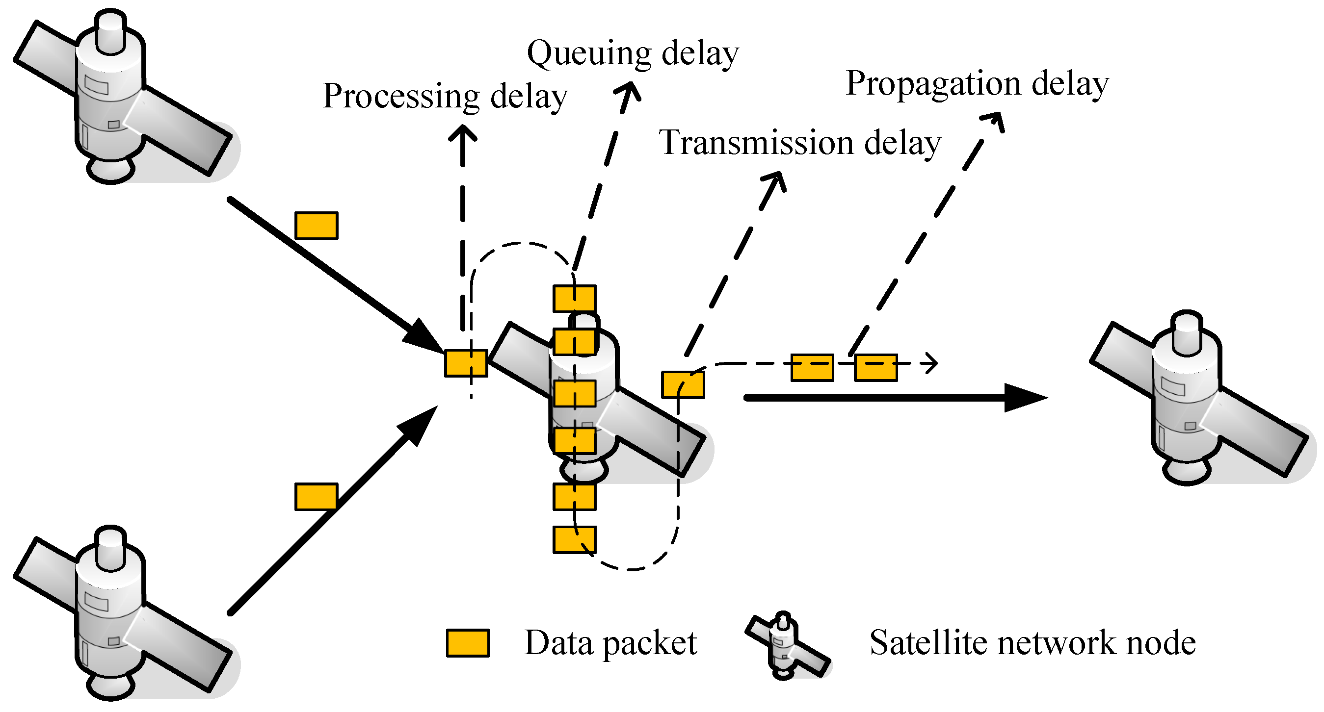
3.2. Satellite Network Delay Prediction Based on GMACC
4. Discussion
5. Conclusions
Author Contributions
Funding
Data Availability Statement
Conflicts of Interest
References
- Widrow, B.; Stearns, S.D. Adaptive Signal Processing; Prentice Hall: Hoboken, NJ, USA, 2008. [Google Scholar]
- Haykin, S. Adaptive Filter Theory; Prentice Hall: Upper Saddle River, NJ, USA, 2002; Volume 4. [Google Scholar]
- Rousseeuw, P.J.; Leroy, A.M. Robust Regression and Outlier Detection; John Wiley & Sons: Hoboken, NJ, USA, 2005; Volume 589. [Google Scholar]
- Zou, Y.; Chan, S.C.; Ng, T.S. Least mean M-estimate algorithms for robust adaptive filtering in impulse noise. IEEE Trans. Circuits Syst. II Analog. Digit. Signal Process. 2000, 47, 1564–1569. [Google Scholar]
- Chan, S.C.; Zou, Y.X. A recursive least M-estimate algorithm for robust adaptive filtering in impulsive noise: Fast algorithm and convergence performance analysis. IEEE Trans. Signal Process. 2004, 52, 975–991. [Google Scholar] [CrossRef]
- Tahir Akhtar, M. Fractional lower order moment based adaptive algorithms for active noise control of impulsive noise sources. J. Acoust. Soc. Am. 2012, 132, EL456–EL462. [Google Scholar] [CrossRef] [Green Version]
- Navia-Vazquez, A.; Arenas-Garcia, J. Combination of recursive least p-norm algorithms for robust adaptive filtering in alpha-stable noise. IEEE Trans. Signal Process. 2011, 60, 1478–1482. [Google Scholar] [CrossRef]
- Principe, J.C. Information Theoretic Learning: Renyi’s Entropy and Kernel Perspectives; Springer Science & Business Media: Berlin, Germany, 2010. [Google Scholar]
- Singh, A.; Principe, J.C. A closed form recursive solution for maximum correntropy training. In Proceedings of the 2010 IEEE International Conference on Acoustics, Speech and Signal Processing, Dallas, TX, USA, 14–19 March 2010; pp. 2070–2073. [Google Scholar]
- Zhao, S.; Chen, B.; Principe, J.C. Kernel adaptive filtering with maximum correntropy criterion. In Proceedings of the 2011 International Joint Conference on Neural Networks, San Jose, CA, USA, 31 July–5 August 2011; pp. 2012–2017. [Google Scholar]
- He, Y.; Wang, F.; Yang, J.; Rong, H.; Chen, B. Kernel adaptive filtering under generalized maximum correntropy criterion. In Proceedings of the 2016 International Joint Conference on Neural Networks (IJCNN), Vancouver, BC, Canada, 24–29 July 2016; pp. 1738–1745. [Google Scholar]
- Hakimi, S.; Abed Hodtani, G. Generalized maximum correntropy detector for non-Gaussian environments. Int. J. Adapt. Control Signal Process. 2018, 32, 83–97. [Google Scholar] [CrossRef]
- Zhao, J.; Zhang, H. Kernel recursive generalized maximum correntropy. IEEE Signal Process. Lett. 2017, 24, 1832–1836. [Google Scholar] [CrossRef]
- Seth, S.; Principe, J.C. Compressed signal reconstruction using the correntropy induced metric. In Proceedings of the 2008 IEEE International Conference on Acoustics, Speech and Signal Processing, Las Vegas, ND, USA, 31 March–4 April 2008; pp. 3845–3848. [Google Scholar] [CrossRef]
- Liu, W.; Pokharel, P.P.; Principe, J.C. Correntropy: Properties and Applications in Non–Gaussian Signal Processing. IEEE Trans. Signal Process. 2007, 55, 5286–5298. [Google Scholar] [CrossRef]
- Yue, P.; Qu, H.; Zhao, J.; Wang, M. An Adaptive Channel Estimation Based on Fixed-Point Generalized Maximum Correntropy Criterion. IEEE Access 2020, 8, 66281–66290. [Google Scholar] [CrossRef]
- Ma, W.; Qu, H.; Gui, G.; Xu, L.; Zhao, J.; Chen, B. Maximum correntropy criterion based sparse adaptive filtering algorithms for robust channel estimation under non-Gaussian environments. J. Frankl. Inst. 2015, 352, 2708–2727. [Google Scholar] [CrossRef] [Green Version]
- Ma, W.; Chen, B.; Qu, H.; Zhao, J. Sparse least mean p-power algorithms for channel estimation in the presence of impulsive noise. Signal Image Video Process. 2015, 10, 503–510. [Google Scholar] [CrossRef]
- Yue, P.; Qu, H.; Zhao, J.; Wang, M.; Liu, X. A robust blind adaptive multiuser detection based on maximum correntropy criterion in satellite CDMA systems. Trans. Emerg. Telecommun. Technol. 2019, 30, e3605. [Google Scholar] [CrossRef]
- Liu, X.; Qu, H.; Zhao, J.; Yue, P. Maximum correntropy square-root cubature Kalman filter with application to SINS/GPS integrated systems. ISA Trans. 2018, 80, 195–202. [Google Scholar] [CrossRef] [PubMed]
- Liu, X.; Qu, H.; Zhao, J.; Yue, P.; Wang, M. Maximum Correntropy Unscented Kalman Filter for Spacecraft Relative State Estimation. Sensors 2016, 16, 1530. [Google Scholar] [CrossRef] [PubMed]
- Yue, P.; Qu, H.; Zhao, J.; Wang, M. Newtonian-Type Adaptive Filtering Based on the Maximum Correntropy Criterion. Entropy 2020, 22, 922. [Google Scholar] [CrossRef] [PubMed]
- Takeuchi, I.; Bengio, Y.; Kanamori, T. Robust Regression with Asymmetric Heavy-Tail Noise Distributions. Neural Comput. 2002, 14, 2469–2496. [Google Scholar] [CrossRef] [PubMed]
- You, W.; Guo, Y.; Zhu, H.; Tang, Y. Oil price shocks, economic policy uncertainty and industry stock returns in China: Asymmetric effects with quantile regression. Energy Econ. 2017, 68, 1–18. [Google Scholar] [CrossRef]
- Amudha, R.; Muthukamu, M. Modeling symmetric and asymmetric volatility in the Indian stock market. Indian J. Financ. 2018, 12, 23–36. [Google Scholar] [CrossRef]
- Sun, H.; Yang, X.; Gao, H. A spatially constrained shifted asymmetric Laplace mixture model for the grayscale image segmentation. Neurocomputing 2019, 331, 50–57. [Google Scholar] [CrossRef]
- Chen, B.; Li, Z.; Li, Y.; Ren, P. Asymmetric correntropy for robust adaptive filtering. arXiv 2019, arXiv:1911.11855. [Google Scholar] [CrossRef]
- Elguebaly, T.; Bouguila, N. Finite asymmetric generalized Gaussian mixture models learning for infrared object detection. Comput. Vis. Image Underst. 2013, 117, 1659–1671. [Google Scholar] [CrossRef]
- Nacereddine, N.; Tabbone, S.; Ziou, D.; Hamami, L. Asymmetric Generalized Gaussian Mixture Models and EM Algorithm for Image Segmentation. In Proceedings of the 2010 20th International Conference on Pattern Recognition, Istanbul, Turkey, 23–26 August 2010; pp. 4557–4560. [Google Scholar] [CrossRef]
- Nandi, A.K.; Mämpel, D. An extension of the generalized Gaussian distribution to include asymmetry. J. Frankl. Inst. 1995, 332, 67–75. [Google Scholar] [CrossRef]
- Lasmar, N.E.; Stitou, Y.; Berthoumieu, Y. Multiscale skewed heavy tailed model for texture analysis. In Proceedings of the 2009 16th IEEE International Conference on Image Processing (ICIP), Cairo, Egypt, 7–10 November 2009; pp. 2281–2284. [Google Scholar] [CrossRef] [Green Version]
- Berner, J.B.; Bryant, S.H.; Kinman, P.W. Range Measurement as Practiced in the Deep Space Network. Proc. IEEE 2007, 95, 2202–2214. [Google Scholar] [CrossRef]
- Yue, P.C.; Qu, H.; Zhao, J.H.; Wang, M.; Wang, K.; Liu, X. An inter satellite link handover management scheme based on link remaining time. In Proceedings of the 2016 2nd IEEE International Conference on Computer and Communications (ICCC), Chengdu, China, 14–17 October 2016; pp. 1799–1803. [Google Scholar]
- Chen, B.; Xing, L.; Liang, J.; Zheng, N.; Principe, J.C. Steady-state mean-square error analysis for adaptive filtering under the maximum correntropy criterion. IEEE Signal Process. Lett. 2014, 21, 880–884. [Google Scholar]
- Wang, W.; Zhao, J.; Qu, H.; Chen, B.; Principe, J.C. Convergence performance analysis of an adaptive kernel width MCC algorithm. AEU-Int. J. Electron. Commun. 2017, 76, 71–76. [Google Scholar] [CrossRef]
- Qu, H.; Shi, Y.; Zhao, J. A Smoothed Algorithm with Convergence Analysis under Generalized Maximum Correntropy Criteria in Impulsive Interference. Entropy 2019, 21, 1099. [Google Scholar] [CrossRef] [Green Version]
- Nichols, K.; Jacobson, V. Controlling Queue Delay. Commun. ACM 2012, 55, 42–50. [Google Scholar] [CrossRef]
- Chang, C.S. Stability, queue length, and delay of deterministic and stochastic queueing networks. IEEE Trans. Autom. Control 1994, 39, 913–931. [Google Scholar] [CrossRef] [Green Version]
- Trindade, A.A.; Zhu, Y.; Andrews, B. Time series models with asymmetric Laplace innovations. J. Stat. Comput. Simul. 2010, 80, 1317–1333. [Google Scholar] [CrossRef]
- Arnold, M.; Milner, X.; Witte, H.; Bauer, R.; Braun, C. Adaptive AR modeling of nonstationary time series by means of Kalman filtering. IEEE Trans. Biomed. Eng. 1998, 45, 553–562. [Google Scholar] [CrossRef]
- Etter, D.M.; Kuncicky, D.C.; Hull, D.W. Introduction to MATLAB; Prentice Hall: Hoboken, NJ, USA, 2002. [Google Scholar]
- Janicki, A.; Weron, A. Simulation and Chaotic Behavior of Alpha-Stable Stochastic Processes; CRC Press: Boca Raton, FL, USA, 2019. [Google Scholar]
- Chen, B.; Xing, L.; Zhao, H.; Zheng, N.; Principe, J.C. Generalized correntropy for robust adaptive filtering. IEEE Trans. Signal Process. 2016, 64, 3376–3387. [Google Scholar] [CrossRef] [Green Version]
- Liu, C.; Jiang, M. Robust adaptive filter with lncosh cost. Signal Process. 2020, 168, 107348. [Google Scholar] [CrossRef]
- Huber, P.J. Robust Statistics; John Wiley & Sons: Hoboken, NJ, USA, 2004; Volume 523. [Google Scholar]


| Algorithm | Number of Additions and Subtractions | Number of Multiplications and Divisions | Number of Exponentiations |
|---|---|---|---|
| LMS | n + 1 | n + 1 | 0 |
| GMACC | n + 2 | n + 5 | 3 |
| Parameters | Simulation 1 | Simulation 2 | Simulation 3, 4, and 5 |
|---|---|---|---|
| Variance | 1 | 1 | 0.25 |
| Shape parameter | 1.98 | 2 | 1.98 |
| Skewness parameter | 0 | 0.4 | 0.3 |
| Scale parameter | 0.2 | 0.2 | 0.2 |
| Location parameter | 0 | 0 | 0 |
| Algorithms | Step Size | Kernel Width | Shape Parameter | MSD (dB) | MSD (dB) | ||
|---|---|---|---|---|---|---|---|
| LMS | 0.09 | - | - | - | - | 30.3309 | −24.4518 |
| MCC | 0.085 | 1 | - | - | - | −24.6445 | −24.7447 |
| MACC | 0.1 | - | 1 | 1 | - | −23.9127 | −24.4624 |
| GMACC | 0.12 | - | 1 | 1 | 1 | −22.8181 | −24.0996 |
| GMACC | 0.11 | - | 1 | 1 | 1.5 | −23.5233 | −24.2051 |
| GMACC | 0.098 | - | 1 | 1 | 2.5 | −23.9438 | −24.4324 |
| GMACC | 0.095 | - | 1 | 1 | 3 | −23.9906 | −24.4935 |
| Algorithms | Step Size | Kernel Width | Steady-State MSD (dB) | ||
|---|---|---|---|---|---|
| LMS | 0.67 | - | - | - | - |
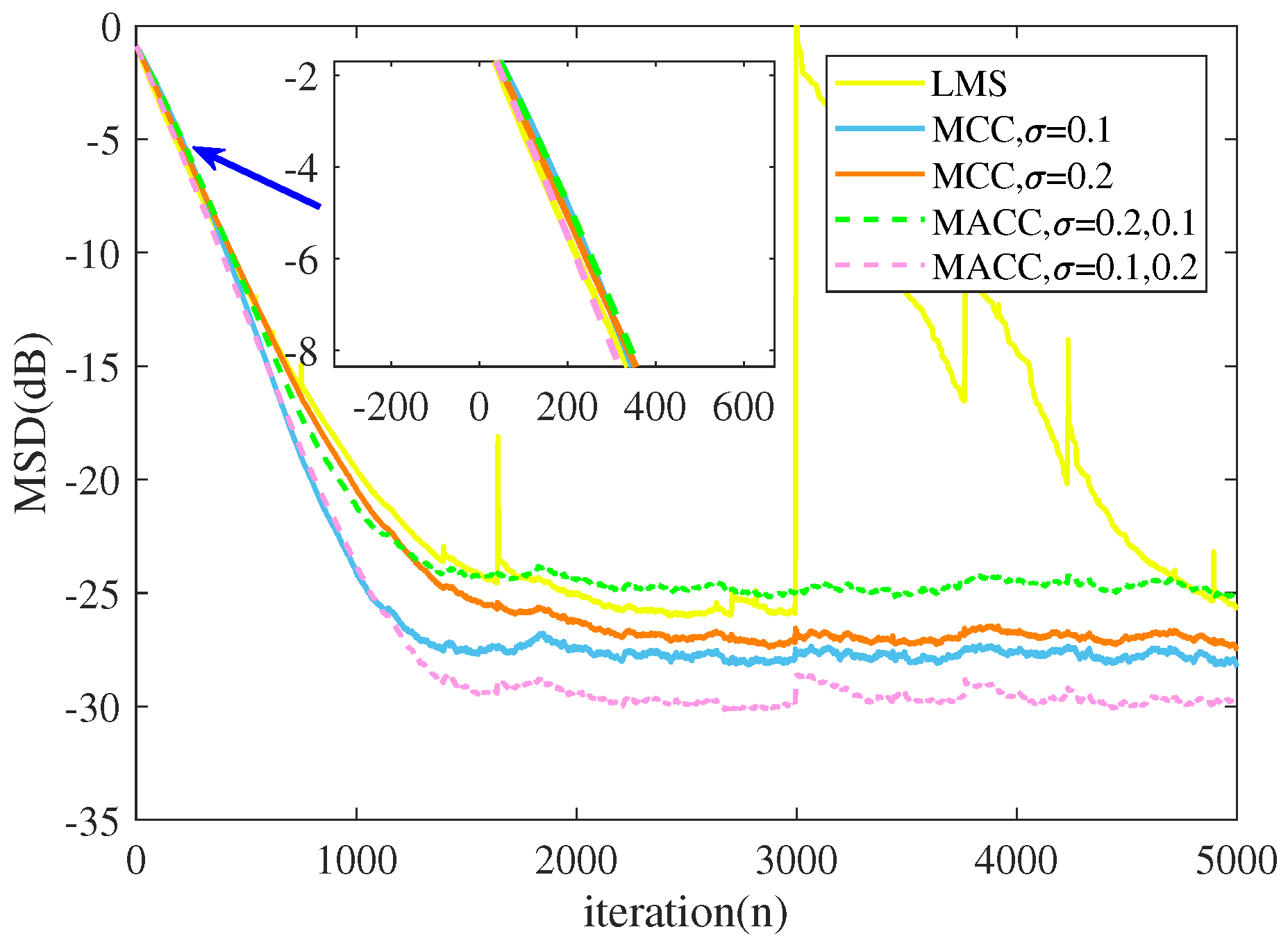
| MCC | 1.39 | 0.1 | - | - | −27.7406 |
| MCC | 0.8 | 0.2 | - | - | −27.0129 |
| MACC | 1.2 | - | 0.2 | 0.1 | −24.7491 |
| MACC | 0.96 | - | 0.1 | 0.2 | −29.6021 |
| Algorithms | Step Size | Kernel Width | Shape Parameter | (Huber) | p (Lp-Norm) | (Llncosh) | MSD (dB) |
|---|---|---|---|---|---|---|---|
| LMS | 1.2 | - | - | - | - | - | 50.6474 |
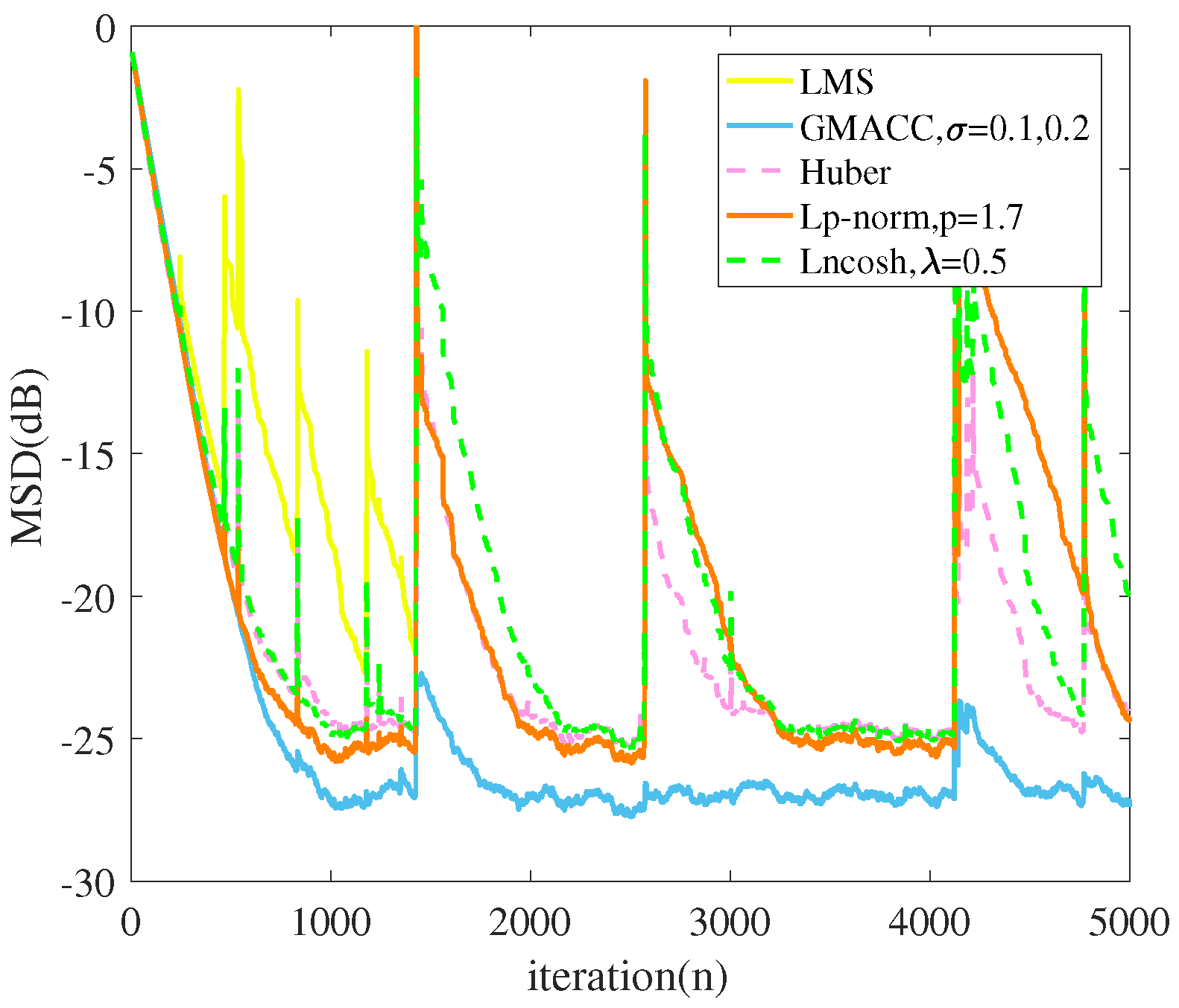
| GMACC | 1.5 | 0.1, 0.2 | 2.25 | - | - | - | −26.3724 |
| Huber | 1.3 | - | - | 1 | - | - | −21.7201 |
| Lp-norm | 0.77 | - | - | - | 1.7 | - | −16.7295 |
| Llncosh | 2.5 | - | - | - | - | 0.5 | −17.8793 |
Publisher’s Note: MDPI stays neutral with regard to jurisdictional claims in published maps and institutional affiliations. |
© 2022 by the authors. Licensee MDPI, Basel, Switzerland. This article is an open access article distributed under the terms and conditions of the Creative Commons Attribution (CC BY) license (https://creativecommons.org/licenses/by/4.0/).
Share and Cite
Qu, H.; Wang, M.; Zhao, J.; Zhao, S.; Li, T.; Yue, P. Generalized Asymmetric Correntropy for Robust Adaptive Filtering: A Theoretical and Simulation Study. Remote Sens. 2022, 14, 3677. https://doi.org/10.3390/rs14153677
Qu H, Wang M, Zhao J, Zhao S, Li T, Yue P. Generalized Asymmetric Correntropy for Robust Adaptive Filtering: A Theoretical and Simulation Study. Remote Sensing. 2022; 14(15):3677. https://doi.org/10.3390/rs14153677
Chicago/Turabian StyleQu, Hua, Meng Wang, Jihong Zhao, Shuyuan Zhao, Taihao Li, and Pengcheng Yue. 2022. "Generalized Asymmetric Correntropy for Robust Adaptive Filtering: A Theoretical and Simulation Study" Remote Sensing 14, no. 15: 3677. https://doi.org/10.3390/rs14153677
APA StyleQu, H., Wang, M., Zhao, J., Zhao, S., Li, T., & Yue, P. (2022). Generalized Asymmetric Correntropy for Robust Adaptive Filtering: A Theoretical and Simulation Study. Remote Sensing, 14(15), 3677. https://doi.org/10.3390/rs14153677