Abstract
Shanghai has gained much attention in terms of air quality research owing to its importance to economic capital and its huge population. This study utilizes ground-based remote sensing instrument observations, namely by Multiple AXis Differential Optical Absorption Spectroscopy (MAX-DOAS), and in situ measurements from the national air quality monitoring platform for various atmospheric trace gases including Nitrogen dioxide (NO2), Sulfur dioxide (SO2), Ozone (O3), Formaldehyde (HCHO), and Particulate Matter (PM; PM10: diameter ≤ 10 µm, and PM2.5: diameter ≤ 2.5 µm) over Shanghai from June 2020 to May 2021. The results depict definite diurnal patterns and strong seasonality in HCHO, NO2, and SO2 concentrations with maximum concentrations during winter for NO2 and SO2 and in summer for HCHO. The impact of meteorology and biogenic emissions on pollutant concentrations was also studied. HCHO emissions are positively correlated with temperature, relative humidity, and the enhanced vegetation index (EVI), while both NO2 and SO2 depicted a negative correlation to all these parameters. The results from diurnal to seasonal cycles consistently suggest the mainly anthropogenic origin of NO2 and SO2, while the secondary formation from the photo-oxidation of volatile organic compounds (VOCs) and substantial contribution of biogenic emissions for HCHO. Further, the sensitivity of O3 formation to its precursor species (NOx and VOCs) was also determined by employing HCHO and NO2 as tracers. The sensitivity analysis depicted that O3 formation in Shanghai is predominantly VOC-limited except for summer, where a significant percentage of O3 formation lies in the transition regime. It is worth mentioning that seasonal variation of O3 is also categorized by maxima in summer. The interdependence of criteria pollutants (O3, SO2, NO2, and PM) was studied by employing the Pearson’s correlation coefficient, and the results suggested complex interdependence among the pollutant species in different seasons. Lastly, potential source contribution function (PSCF) analysis was performed to have an understanding of the contribution of different source areas towards atmospheric pollution. PSCF analysis indicated a strong contribution of local sources on Shanghai’s air quality compared to regional sources. This study will help policymakers and stakeholders understand the complex interactions among the atmospheric pollutants and provide a baseline for designing effective control strategies to combat air pollution in Shanghai.
1. Introduction
Anthropogenic activities are a major source of deterioration in air quality. With advancements in technology, the extent of air quality deterioration has increased manifolds owing to the enhanced fossil fuel combustion by various kinds of transport to meet the modern-day requirements [1,2]. Air pollution has gained much attention in China owing to the fast-paced industrialization, economic growth, urbanization, and massive population. According to the World Health Organization (WHO) standards, only 1% of China’s megacities meets the safe city criteria in terms of air quality [3]. Atmospheric quality directly influences the earth’s radiation budget as well as the ecological environment. It also has pronounced effects on regional climate, agriculture, and human health [4,5].
Sulphur dioxide (SO2), Nitrogen oxides (NOx), and formaldehyde (HCHO) are important constituents of the atmosphere and are known to have a strong influence on air quality and regional climate [6]. NOx comes from a variety of sources, though essentially from electric utilities, combustion processes, transportation, and industry. Photochemical reactions that involve NO2 are vital for tropospheric ozone production [7], which severely impacts air quality and human health. SO2 is a crucial primary atmospheric pollutant that plays an important function in defining the atmospheric chemistry and climate at the regional level. This gas is supposed to be a potential threat to human health as it severely affects human respiratory health [8]. The removal pathways include dry and wet deposition (either as settling with dust or acid rain) or by oxidation, which contributes to the formation of sulphate aerosols [9]. Anthropogenic SO2 emissions generally come from fuel consumption for domestic heating or power generation, etc., in the urban environment, while the minor sources include shipping, oil refining, and metal smelting [10]. Anthropogenic SO2 emissions are usually restricted to the atmospheric boundary layer, whereas the regional emission and transport sources are characterized by the vertical distribution of SO2 in various atmospheric layers.
Formaldehyde (HCHO) is one of the simplest hydrocarbons (HC) in the atmosphere. It has a short life span and comes from the oxidation of VOCs [11,12]. Therefore, the tropospheric variability of HCHO largely depends on VOC oxidation. Direct emissions result from fossil fuel combustion, natural vegetation, and biomass burning [13]. Both HCHO and NO2 are very important trace gas species in the atmosphere and are definitive of the atmospheric chemistry. Complex photochemical reactions involving NOx and VOCs play a substantial role in the formation of tropospheric Ozone (O3) [14]. As an oxidation product of VOCs, HCHO is usually employed as a proxy for VOC reactivity [15] while NO2 concentrations in the troposphere are closely related to NOx [16]. Therefore, the ratio of HCHO to NO2 (RFN) is employed as a proxy to study O3-NOx-VOC sensitivity [5,17,18]. The aforementioned trace gas species, along with other atmospheric trace gas molecules, have been extensively observed by employing Multiple AXis Differential Optical Absorption Spectroscopy (MAX-DOAS) owing to its ubiquity in an urban environment and strong UV absorption [19,20,21,22]. Particulate Matter (PM) is another crucial air pollutant which is classified into PM10 (diameter ≤ 10 µm) and PM2.5 (diameter ≤ 2.5 µm). PM pollution has become a major cause of concern owing to adverse health impacts (e.g., respiratory and cardiovascular diseases) and deterioration in air quality (e.g., haze formation), [23].
Shanghai is called the economic capital of China owing to its huge economic activity and the warm water seaport. It is one of the largest metropolitan areas, with a population of 24.87 million as of 2020 (National Bureau of Statistics of China, 2021). Due to the fast-paced urbanization and industrialization of Shanghai and the surrounding cities, the air quality of the city has deteriorated thereby gaining much attention in terms of air quality and public health research [24]. The aforementioned facts render Shanghai a prime location for the continuous monitoring of air pollution to assist in the policymaking process and joint control strategies to cap anthropogenic emissions. The continuous monitoring of trace gas species is crucial not only towards understanding environmental footprints but also their social implications.
Ozone (O3) is a species of concern with respect to atmospheric pollution across the globe). A series of regulations and strategies were issued by the Chinese government to mitigate air pollution. For example, the Air Pollution Prevention Action Plan [25,26] and the Win the Blue Sky three-year action plan, in 2013 and 2018, respectively, focused on reducing the concentration of PM2.5 [27,28]. These efforts were effective, with a recorded reduction in annual mean concentrations of PM2.5 from 74 mg/m3 to 39 mg/m3 for 31 provincial capitals during 2013–2018 (http://english.mee.gov.cn/ (accessed on 28 February 2022)). The average annual concentrations of other pollutants including NO2, SO2, CO, and PM10 declined by 9.7%, 54.1%, 28.2%, and 27.8%, respectively, over 74 big cities, with O3 concentration observed to increase by a whopping 20.4% [12,26,29,30]. Hence, O3 production strongly depends on the ratio of VOCs and NOx [31]. Previous strategies to combat O3 pollution focused on controlling NOx emissions [32], while a higher O3 concentration occurs in a VOC-limited regime [33]. Therefore, this study may serve as a guide for government agencies regarding the control policies of O3 pollution based on HCHO/NO2. O3 sensitivity studies over Shanghai have been reported in the literature; however, these studies were limited only to a specific time period of the year or a single season [11,20], creating gaps in holistic analysis and understanding. To the author’s best knowledge, this is the first study that tries to analyze O3 sensitivity across the year with ground-based observations while emphasizing the seasonal trends of other atmospheric species including HCHO, SO2, and NO2 species.
For the current study, MAX-DOAS observations at a suburban site in Shanghai were utilized to evaluate the variation in trends of different trace gas species, including SO2, NO2, and HCHO, from June 2020 to May 2021. The organization of the study is as follows: Section 2 describes the study site, instrument specifications, and the DOAS methodology used for the analysis and retrieval. The additional datasets used for further assessments and analysis have also been referenced. A time series of daily mean concentrations for HCHO, NO2, and SO2 was generated (Section 3.1) based on the described methodology, which provided the basis for performing additional analysis including the monthly, seasonal, and diurnal variations (Section 3.2). The study was complemented by the dependence on meteorology (including temperature and humidity; Section 3.3) as well as the enhanced vegetation index (EVI) (Section 3.4), which was followed by sensitivity analysis for tropospheric Ozone (O3) production (Section 3.5). The interdependence of different pollutants using in situ measurements was also studied (Section 3.6). Finally, the potential source contribution function (PSCF) was analyzed (Section 3.7), succeeded by a scientific conclusion.
2. Materials and Methods
2.1. Observation Site
Shanghai is one of the largest cities of China in terms of population and economic activities, with one of the world’s largest container ports. The city has witnessed several episodes of high pollution to date which are attributed to massive fossil fuel combustion to meet the energy and transport requirements of the city’s huge population. The observations for the current study were made at the Shanghai Nanhui Environment Monitoring Station (121.807003°E, 31.054963°N), which is a suburban site in Shanghai located away from the city center, near to shore, and south of Pudong International Airport by a distance of 11 km (Figure 1).
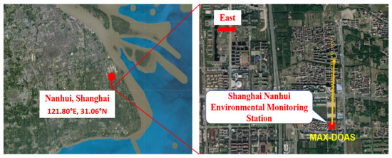
Figure 1.
The region surrounding the measurement station (31.05°N, 121.81°E) is shown by the topography map (Google Maps). The arrow points towards the direction of the telescope of the Multiple AXis Differential Optical Absorption Spectroscopy (MAX-DOAS) instrument.
2.2. MAX-DOAS Instrument
The ground based remote sensing instrument MAX-DOAS used in this study entails a scanning telescope which is governed by a stepping motor, a spectrometer (Ocean Optics, Orlando, FL, USA, QE65 Pro), and a computer that acts as an operating system. Optical fiber has been employed in the telescope to collect scattered sunlight. The spectrometer is geared up with a charged coupled device (CCD) detector (with a resolution of 1044 Horizontal × 64 vertical and cooling up to −15 °C) which has been used for the measurements in wavelength ranging from 300 nm to 480 nm. This spectrometer has a spectral resolution of 0.5 nm full-width half maximum (FWHM). The telescope is directed north clockwise at an azimuthal angle of 2° to avoid direct sunlight and is capable of scanning at ten different elevation angles (EA). The sequence includes measurements 2°, 3°, 5°, 7°, 9°, 12°, 15°, 20°, 30°, 45°, and 90°. The whole cycle of scanning takes around five minutes to complete. Background measurements were taken each night, and the signal for the dark current was automatically extracted from them. Validation of MAX-DOAS instrument has been performed by several previously reported studies [20,22] and shows good agreement with both space-based and ground-based trace gas monitoring instruments. The position of the instrument is shown in Figure 1.
2.2.1. DOAS Analysis
Accurate column measurements for the trace gases in the atmosphere are possible only because the MAX-DOAS instrument can measure dispersed sunlight at several elevation angles, known as EVAs. A Fraunhofer reference spectrum was selected as the zenith measurements for each measurement sequence, which was then subtracted from the off-zenith spectrum to obtain differential slant column densities (DSCDs). DSCDs refer to the integrated number density for any trace gas along the effective light path. The process essentially minimizes the stratospheric interference to the tropospheric measurements [19]. The DOAS technique is used to recover DSCDs of SO2, NO2, and HCHO from the obtained spectra [34], which involves the analysis of the recorded spectra utilizing the QDOAS software version 3.2 (http://uv-vis. aeronomie.be/software/QDOAS/ (accessed on 17 September 2021)). The configuration of the DOAS retrievals is based on previous studies [35,36] and the MAD-CAT campaign (http://joseba.mpchmainz.mpg.de/mad_analysis.htm (accessed on 17 September 2021)). Table 1 describes the configurations for SO2, NO2, and HCHO retrieval from DOAS, where “parameters” refer to the absorption cross-sections of interfering compounds and “data source” refers to the source and temperature at which absorption cross-sections are measured. A high-resolution solar spectrum was used to calibrate the wavelength [37]. Owing to the scattering processes in the atmosphere, the quality of data is likely to be impacted. To avoid this, certain filters are applied to maintain quality. The data with a root mean square (RMS) greater than 0.002 and a solar zenith angle greater than 75 were filtered out for this study. The RMS represents the average error in spectral analysis for MAX-DOAS. The detection limit for DSCDs is estimated based on the typical DOAS fit errors of discrete species under characteristic measurement circumstances.

Table 1.
Retrieval settings for trace gases spectral analysis.
2.3. Ancillary Data
The Aqua-Moderate Resolution Imaging Spectrometer (MODIS) has been employed here to obtain the vegetation index, which was used as a proxy for biogenic emission sources. MODIS vegetation index products are unique as they provide spatial as well as temporal comparisons for the vegetation cover over any area. Enhanced vegetation index (EVI) at 250 m resolution from the Aqua-MODIS vegetation product (MYD13Q1 V006) was used to support our analysis.
The daily mean concentrations were taken for the criteria pollutants, including SO2, NO2, O3, PM10, and PM2.5, from June 2020 to May 2021 from China’s air quality online monitoring and analysis platform (downloaded from: https://www.aqistudy.cn/ (accessed on 25 September 2021)).
Meteorological data including temperature, wind speed, relative humidity, and wind direction were obtained from the automatic weather station installed at Pudong International airport to determine the impact of meteorological parameters on pollutant concentrations.
2.4. PSCF Analysis
Backward trajectory analysis was performed to determine the origin of air masses using the Hybrid Single-Particle Lagrangian Integrated Trajectory (HYSPLIT) model developed by National Oceanic and Atmospheric Administration (NOAA) [43]. The model offers a comprehensive understanding of the transport of air masses, their dispersion, and their chemical transformation [44], along with highlighting the likely causes of aerosol pollutants which affect the air quality. The Potential Source Contribution Function (PSCF) analysis was integrated with the HYSPLIT back trajectory model and daily NO2, SO2, and HCHO measurements over a grid of 0.5 × 0.5 degrees. The HYSPLIT model backward trajectory at a height of 500 m above the ground level (AGL) for 72-h was computed every 6-h by using the Global Data Assimilation System (GDAS) meteorological data at a spatial resolution of 1° × 1° (accessible at ftp://arlftp.arlhq.noaa.gov/pub/archives/gdas1 (accessed on 23 December 2021)) at seasonal scales from June 2020 to May 2021.
The height 500 m is the estimated height of the boundary layer; therefore, it is reported to have been very useful when used as AGL for the trajectory analysis [45,46]. Assuming that the endpoint for the trajectory is located inside the grid (i,j), the PSCF value was enumerated. It was also assumed that the trajectory collects pollutants coming from diverse sources of emission within that cell (i,j). Therefore, by definition, the PSCF value is the conditional probability which is definitive of the potential contribution of extraordinary pollutant loading at the receptor location for the grid cells. Equation (1) defines the calculation of the PSCF value for the ijth grid cell:
where nij signifies the frequency of endpoints falling or passing through the ijth cell and mij represents the frequency of endpoints in the ijth cell that have a higher pollutant load than the 24-h Air Quality Standards. Small nij may cause uncertainty in the calculations and results. Multiplying an arbitrary weight function Wi,j to the PSCF greatly reduces this uncertainty. Equation (2) gives the weight function for the current analysis:
Here, n signifies the average numeral of endpoints for each cell, computed for each cell with a minimum of one endpoint. Equation (3) expresses the Weighted PSCF, which is given as:
3. Results and Discussion
3.1. MAX-DOAS Observations
Figure 2 shows the time series for daily averaged HCHO, SO2, and NO2 and monthly averaged concentrations, which are represented by red dots. There are certain gaps in the observations owing to instrumental error and maintenance as well as the quality filters. The data, which qualified a certain quality standard (mentioned under Section 2.2.1), were used for the analysis. The daily HCHO minimum, maximum, and mean concentrations of 1.26 × 10¹⁶ molecules/cm2, 6.31 × 10¹⁶ molecules/cm2, and 2.48 × 10¹⁶ molecules/cm2 were observed, respectively (Figure 2a). Minimum SO2 concentration was observed to be 1.92 × 10¹⁶ molecules/cm2, while 1.57 × 10¹⁷ molecules/cm2 was the peak value observed depicting an average of 3.97 × 10¹⁶ molecules/cm2 (Figure 2b). The average NO2 remained to be 7.51 × 10¹⁶ molecules/cm2 with a minimum of 5.16 × 10¹⁵ molecules/cm2 and a maximum of 2.24 × 10¹⁷ molecules/cm2 (Figure 2c). HCHO shows higher values during summer, with peak values occurring during August, while both NO2 and SO2 depicted opposite trends with peaks in January. This trend complies with the previous studies reported for these species in different regions [6,47,48,49].
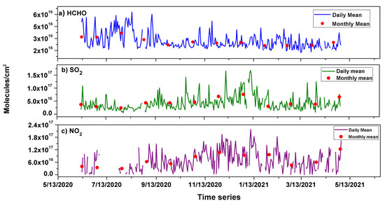
Figure 2.
Daily and monthly averages of (a) HCHO, (b) SO2, and (c) NO2 from June 2020 to May 2021.
3.2. Seasonal Variations and Diurnal Cycles
The seasonal variation in pollutant concentration is meticulously connected to meteorological conditions in conjunction with the characteristics of diverse sources of emission. The diurnal variability of any pollutant is affected by the solar intensity, a planetary boundary layer (PBL), emission sources, and wind pattern [50]. Seasonal variations in HCHO, NO2, and SO2 over suburban Shanghai are depicted in Figure 3. HCHO depicted the highest values during summer followed by autumn, winter, and spring. The surge in HCHO emissions for the summer months is said to be the result of its production by photochemical reactions and biomass burning, while the emissions from biogenic sources during the growing season, i.e., spring and autumn, also contribute towards its emissions [51]. The impact of biogenic emissions has been discussed separately under Section 3.5. For SO2 and NO2, however, the opposite trend was observed with the highest values observed during winter, followed by spring, autumn, and summer. These characteristics are already well recognized and reported over various metropolitan areas in China [52,53] and in other regions [46].
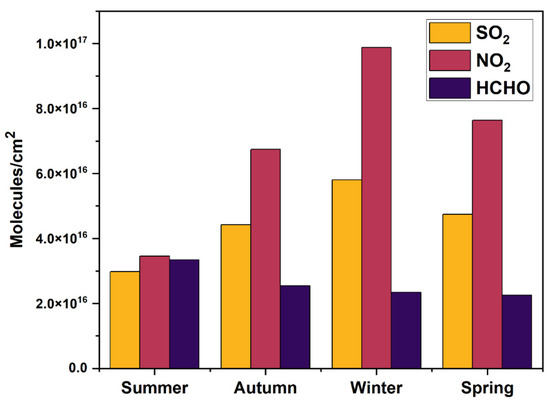
Figure 3.
Seasonal variation in SO2, HCHO, and NO2 over Shanghai.
Higher NO2 in winters is associated with a longer atmospheric lifetime and higher emission during winters owing to domestic heating and power consumption [51]. A high mixing ratio and less solar intensity during winters are associated with a higher atmospheric lifetime of NO2 compared to summer. Solar intensity is crucial towards initiating the breakdown reactions for NO2; consequently, NO2 persists for a longer period in the atmosphere during winter compared to summer [46]. Less turbulence and less surface heating in winter, which are attributed to lower solar intensity, cause the formation of a stable boundary layer with a low height. Moreover, owing to the effect of local heating close to the top of the boundary layer, the atmospheric stability is increased owing to high concentrations of light-absorbing aerosols, especially black carbon (BC), which causes the boundary layer height (BLH) to lower further [54]. Shallow BLH, coupled with lower wind speed, causes stable atmospheric conditions and is crucial towards restricting the transport of aerosols, which further causes the aerosol buildup and enrichment of near-surface particle concentrations. Consequently, the lifetime of anthropogenic aerosols such as those coming from the combustion of fossil fuel and certain industrial and urban activities may be increased [46,55].
Transport from the highly polluted areas is essentially crucial towards determining the seasonal behavior of SO2, especially in winters, owing to its long residence time in the atmosphere (<1 h to 2 weeks, as reported in the literature [56], owing to the fact that elongated residence time will allow for transport of greater distance with turbulence). In summary, the removal pathway including oxidation by OH radicals is crucial in defining the seasonality of NO2 which depicts maxima in winter and minima in summer [57]. The seasonality of SO2 is also partly linked to a similar removal mechanism [58], while heterogeneous reactions play a further role [59]. HCHO seasonality trends are the opposite owing to enhanced sunlight in summer months, which enhances its formation by the photochemical reactions [60]. Figure 3 depicts seasonally averaged SO2, HCHO, and NO2 for Shanghai from June 2020 to May 2021. The average concentrations during winter remained to be 5.63 × 10¹⁶ molecules/cm2, 2.14 × 10¹⁶ molecules/cm2, and 9.71 × 10¹⁶ molecules/cm2 for SO2, HCHO, and NO2, respectively. For autumn, the concentrations were observed to be 4.80 × 10¹⁶ molecules/cm2, 2.47 × 10¹⁶ molecules/cm2, and 7.63 × 10¹⁶ molecules/cm2, respectively, while, for spring, the seasonally averaged concentrations were 4.20 × 10¹⁶ molecules/cm2, 1.94 × 10¹⁶ molecules/cm2, and 6.98 × 10¹⁶ molecules/cm2, respectively. For summers, the seasonally averaged concentrations depicted 2.98 × 10¹⁶ molecules/cm2, 3.40 × 10¹⁶ molecules/cm2, and 3.17 × 10¹⁶ molecules/cm2 for SO2, HCHO, and NO2.
The diurnal variations in HCHO depicted an increase in concentrations from morning to noon and declining from afternoon to evening (Figure 4a). Only a weak cycle is visible for autumn and winter (black and green curves), and an opposite or no clear trend is observed for summer and spring (blue and red curves). This is attributed to the enhanced photolytic oxidation of VOCs to form HCHO with an increase in light intensity during the day [51]. A similar diurnal trend has been observed in different regions in various previously published studies [6,60]. The seasonal variation in HCHO diurnal trends shows peak value during the summer, followed by autumn, winter, and spring. A similar diurnal trend for different seasons has been reported by other studies [13]. SO2 shows an opposite diurnal trend as that of HCHO (Figure 4b), with peak values occurring in the morning and evening. This might be because there is enhanced anthropogenic activity during morning and evening hours, with more vehicle flux consuming more fuel and generating more pollutant gases [61]. The diurnal variation in SO2 concentrations can also be explained by the strengthened emission sources during this time [62,63]. The results suggest strong seasonality in SO2 concentrations with peak values occurring in winter, followed by spring, autumn, and summer. Similar diurnal trends for different seasons have been reported earlier [64].
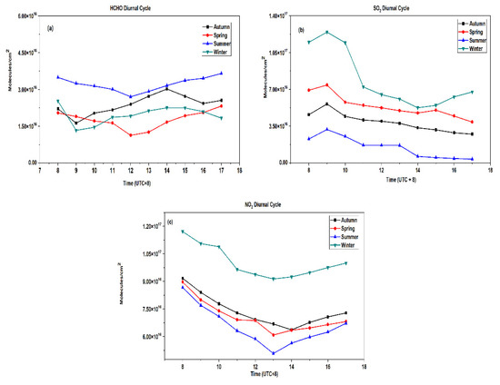
Figure 4.
Diurnal cycle of (a) HCHO, (b) SO2, and (c) NO2 for different seasons as obtained from MAX-DOAS observations.
A similar diurnal trend was observed for NO2 (Figure 4c). Owing to an increase in solar intensity during the daytime, photolytic oxidation is enhanced, which acts as a sink for NO2 [61], justifying a sharp decline in NO2 concentrations, especially in summers when sunlight intensity is highest of all the seasons. Moreover, higher levels of NOx during morning and evening hours can be attributed to low PBL, which weakens the mixing process for air pollutants, while lower pollutant levels during the day result from high PBL, which increases the diffusion of pollutants in the atmosphere. Similar results are reported by earlier studies [61,65]. The seasonal diurnal trend for NO2 shows the highest values in winter followed by autumn, spring, and summer. This trend complies with the studies reported earlier [64,66].
3.3. Relationship with Meteorological Parameters
Aerosol and trace gas distributions along with the residence time and chemical behavior are largely affected by the meteorological settings over the vicinity [5,6]. Figure 5 shows the time series of temperature (°C), relative humidity (RH%), and wind speed (m/s) for the study period. These parameters are pivotal in determining trace gas concentrations.
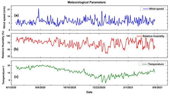
Figure 5.
Time series for (a) wind speed (m/s), (b) relative humidity (%), and (c) temperature (°C).
The correlation coefficient of weekly mean SO2, NO2, and HCHO with RH is shown in Figure 6A. As the MAX-DOAS instrument is capable of observation during daytime hours, only daytime values for temperature and RH were averaged in order to make correlations. HCHO shows a slight positive correlation coefficient of 0.42 (Figure 6(Aiii)), suggesting an increase in HCHO concentration with enhanced humidity, while both NO2 and SO2 have a negative correlation coefficient of 0.65 (Figure 6(Ai)) and 0.72 (Figure 6(Aii)) with RH, respectively, implying that both NO2 and SO2 concentrations decline at high RH, or that both SO2 and NO2 can have higher concentrations at low RH and that this is the reason higher concentrations were observed during winter compared to summer (please see Section 3.2). This is probably because of the OH oxidation of SO2 and NO2 at a higher humidity, where NOx removal mechanisms are particularly affected by the increase in humidity [67]. It is conceivable that aerosol particles in the atmosphere will swell with increasing humidity, and thus the contact area for gas-particle exchange will increase. Therefore, gaseous species (i.e., SO2 and NO2) can more frequently enter the particle phase and will be removed. Liu, Zhou, and Lu, 2020 [68], reported a similar correlation coefficient for SO2 and NO2 with RH.
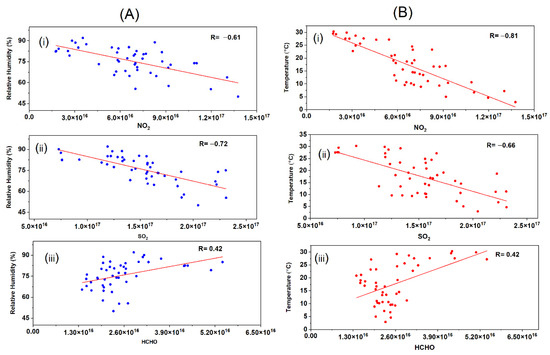
Figure 6.
Relationship of RH (A) and T (B) with weekly averaged (i) NO2, (ii) SO2, and (iii) HCHO.
Temperature is another crucial factor in determining trace gas concentration and atmospheric chemistry. HCHO shows an enhanced concentration with increased temperature (R = 0.52; Figure 6(Biii)), suggesting that the photo-oxidation of VOCs is the main source of HCHO formation [6,69]. NO2 and SO2 depicted a negative correlation coefficient of 0.81 and 0.66 (Figure 6(Bi,ii)) with temperature, respectively. This is because an increase in temperature is usually associated with enhanced photo intensity, which in turn leads to photolytic degradation of SO2, NO2, and VOCs. HCHO concentrations increase because VOC oxidation is the major source of its formation in the atmosphere [51].
3.4. Impact of Biogenic Emissions
During the growing season (spring to autumn), biogenic emissions tend to have a stronger influence on trace gas chemistry. According to the literature, the relative contribution of biogenic emissions to the overall VOCs is predicted to be about 13% [70]. High-quality spatial and temporal coverage of the vegetation cover can be obtained from the MODIS vegetation index products [71,72,73]. During summer, EVI values were observed to be high, indicating the presence of vegetation. Here, we analyzed the linkage between EVI and the formation of HCHO, NO2, and SO2 to assess the impact of biogenic emissions on the concentrations of these trace gases.
A moderately positive correlation is exhibited by HCHO with EVI (Figure 7a), which is indicative of the fact that the formation of HCHO is associated with the oxidation of isoprene, which is a common VOC [6,74], whereas both NO2 and SO2 depicted a negative correlation (Figure 7b,c), implying that these two species do not come from biogenic sources. Vrekoussis et al. [75] reported an anti-correlation of NO2 with EVI, while Guo et al. [76] argued that SO2 decreases with an increase in vegetation as it enhances the absorbing capability for SO2. In conclusion, HCHO emissions are impacted by anthropogenic as well as biogenic emissions, which are indicated by a moderately positive correlation between the two, whereas both NO2 and SO2 come from anthropogenic sources. These results are consistent with previous studies [6,75].
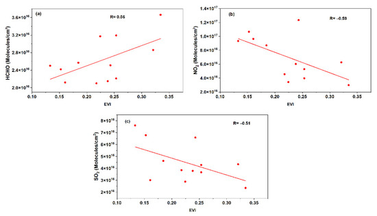
Figure 7.
Relationship of monthly mean (a) HCHO, (b) NO2, and (c) SO2 with monthly mean EVI.
3.5. O3–NOx–VOC Sensitivity
The conditions for O3 formation by VOCs or NOx have broadly been categorized into three regions: (1) a VOC-limited regime, where VOCs are the major precursor for O3 formation; (2) a NOx-limited regime, where the levels of NOx determine the levels of O3; (3) a transition regime, where both NOx and VOC contribute equally towards O3 formation [77]. Several studies have utilized the ratio of HCHO to NO2 (RFN) as a proxy to study the sensitivity of tropospheric O3 formation to these species [20,78]. The linkage between RFN and O3 formation was described by Duncan et al. [76], and the study suggested that the RFN values for the aforementioned regimes where an RFN less than 1 corresponds to a VOC-limited regime, an RFN of more than 2 characterizes an NOx-limited regime, while an RFN value of between 1 and 2 corresponds to transition regimes. Figure 8 shows the RFN for Shanghai over the observation period. For most of the observation period (about 68%), the O3 production remained in the VOC-limited regime. While 20% of the time, the O3 production lay in the transitional regime, and it was NOx-limited for only 12%. These results imply that VOCs are a major player for O3 formation in Shanghai.
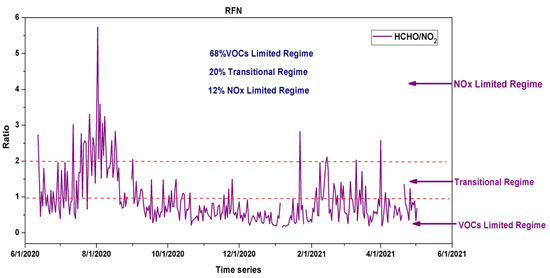
Figure 8.
Daily mean RFN over Shanghai from June 2020 to May 2021.
Further, seasonal variations in RFN were analyzed. Table 2 depicts the mean, standard deviation, minimum, maximum, and median values of RFN for different seasons along with the percentage of O3 formation regimes over Shanghai. The mean value for RFN shows very little variation for winter, spring, and autumn (between 0.63 and 0.73), while, for summer, the mean RFN was observed to be higher (>1.38). This is because significant O3 formation lay in the VOC-NOx-limited regime or transition regime (about 31%) during this season. It is worth noting here that O3 peaks are also observed during the summer season [66]. Yet, O3 formation predominantly remained in the VOC-limited regime for all the seasons. This trend is consistent with previously reported studies [74,79,80].
Table 2.
Seasonal variation in RFN calculated for the analysis of O3 sensitivity.
3.6. Relationship among Different Pollutants
In situ daily mean concentrations were used to study the correlations among five criteria pollutants, including NO2, SO2, O3, PM2.5, and PM10 over the study area for different seasons. Pairwise Pearson’s correlation coefficient was employed for this analysis, which has been depicted in Figure 9. PM2.5 depicted a strongly positive correlation with PM10 for all seasons (R = 0.76 for summer, R = 0.74 for autumn, and R = 0.64 for winter) except during spring, where it showed a weak negative correlation (R = −0.13). This is most likely because of the occurrence of sandstorms in eastern China during the spring months, which substantially enhance PM10 concentrations in the atmosphere [81]. PM2.5 also depicted moderate positive correlations with primary pollutants (NO2 and SO2) for all the seasons (R > 0.48 with NO2 and R > 0.34 with SO2 for all seasons). This is indicative of the similar sources of emissions (such as fossil fuel combustion and vehicular exhausts) for these pollutants. PM10 also depicted weak positive correlations with NO2 and SO2 for all seasons (R > 0.30 for NO2 and R > 0.17 for SO2 for all seasons) except spring, where the correlation between NO2 and PM10 was found to be negative (R = −0.56). This can be attributed to high PM10 content resulting from sandstorms, as stated above. These results are consistent with the findings reported by Sulaymon et al. [81].
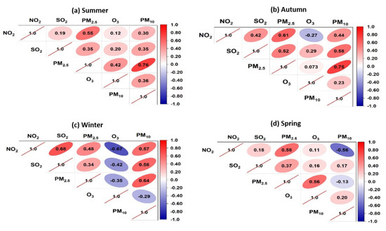
Figure 9.
Pearson’s correlation coefficients among different pollutants for (a) summer, (b) autumn, (c) winter, and (d) spring over Shanghai.
The positive correlation of PM2.5 with SO2 and NO2 is attributed mainly to the coal-fired power plants and huge emissions from traffic [82]. Moreover, it can be argued that the positive correlation of PM (PM10 and PM2.5) with SO2 and NO2 might be because these primary gaseous pollutants act as a precursor for the formation of major components (nitrates and sulfates) of PM [83]. A significantly weak correlation has been observed between NO2 and SO2 for summer (R = 0.19) and spring (R = 0.18) while a moderate correlation was found among the two during autumn (R = 0.42). During winter, however, the correlation between NO2 and SO2 was fairly strong (R = 0.68). These findings indicate varied and multiple sources of emission for these two atmospheric species during different seasons [84]. The correlation of O3 with all other species was found to be negative during winter. During other seasons, however, the correlation was slightly positive except for NO2 (negative during autumn as well) and PM2.5 (fairly positive during spring). Chen et al. [85] reported a negative correlation between PM2.5 and O3 during winter, while a significantly positive correlation was reported for summer over the East China region. The least correlation coefficients of O3 were observed, with NO2 depicting a negative correlation during winter and autumn, while, for spring and summer, the correlation was positive, albeit insignificant. The negative correlation of O3 with NO2 is explained through studying the tropospheric chemistry, where the reaction of O3 with NO leads to the formation of NO2, thereby depleting O3 [86]. Additionally, these results imply that O3 formation over Shanghai mainly lies in the VOC-limited regime. These results comply with previously reported findings [51,87].
3.7. Potential Source Regions of Pollutants
PSCF analysis was based on HCHO, NO2, and SO2, grouped by season (summer; autumn; winter; spring), over Shanghai, using 72-h back trajectories attained from the NOAA HYSPLIT model and ground-based data to detect the potential source areas of HCHO, NO2, and SO2. The HYSPLIT-derived back-trajectories over Shanghai were used to compute PSCF for each air pollutant and show the major likely sources of pollution. It is important to mention that the significant differences between sources and seasons were observed over Shanghai. The high values of PSCF (>0.50) in summer indicate that the contribution of local sources (e.g., Anhui, Fujian, Guangdong, Guangxi, Hainan, Hong Kong, Jiangsu, Jiangxi, Macao, Shandong, and Zhejiang) is much stronger than outside sources (Myanmar and Vietnam), which is more observable for HCHO than NO2 and SO2 concentrations (Figure 10a). These local sources of HCHO concentration more significantly affect the air quality of Shanghai than regional sources. As in summer, local sources (i.e., Anhui, Beijing, Hebei, Hubei, Inner Mongolia, Jiangsu, Jiangxi, Shandong, and Zhejiang) of the three concentrations (HCHO, NO2, and SO2) also substantially affect the autumn (Figure 10b) air quality over Shanghai more than distant regional sources such as Mongolia do, as indicated by the higher values of PSCF (>0.50). In winter, the contribution of local sources (e.g., Anhui, Beijing, Fujian, Guangdong, Guangxi, Hebei, Henan, Hubei, Inner Mongolia, Jiangsu, Jiangxi, Liaoning, Shandong, Shanxi, Shaanxi, Tianjin, and Zhejiang) is much stronger than outside sources (Mongolia and Russia), which is more observable for NO2 and SO2 than HCHO concentrations (Figure 10c). The springtime air quality over Shanghai is also significantly impacted by local pollution sources (Figure 10d). Overall, the results show that local sources from mainland China are the major contributors of air pollution over Shanghai, with NO2 and SO2 pollution levels being higher in winter than in other seasons, whereas HCHO pollution is higher in summer.
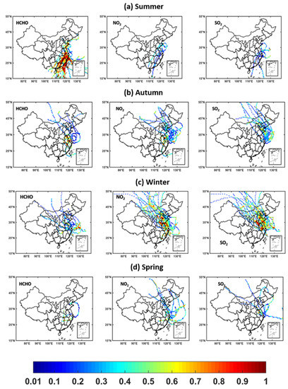
Figure 10.
PSCF analysis based on HCHO, NO2, and SO2, grouped by seasons (a) summer, (b) autumn, (c) winter, and (d) spring over Shanghai: Here, the color bar indicates the weights of the pollution source regions (WPSCF). Regions with WPSCF < 0.4 are termed a low-polluted source regions, regions with WPSCF between 0.4 and 0.5 are considered medium-polluted source regions, while the WPSCF > 0.5 indicate high-polluted source regions.
4. Conclusions
The current study was conducted to monitor various trace gas species over a sub-urban site in Shanghai for one year. Ground-based MAX-DOAS observations were recorded, spanning from June 2020 to May 2021. The spectra were analyzed using QDOAS, and the time series was obtained for HCHO, NO2, and SO2. The results indicated strong seasonality for these trace gas species, with both NO2 and SO2 being higher during winter while HCHO concentrations were higher during the summer season. These results can be explained by the correlation of these species with temperature, where HCHO shows a strong positive correlation (R = 0.78), while both NO2 and SO2 depict a negative correlation (R = −0.66 and R = −0.57, respectively). Similar correlations have been found with RH, where an increase in humidity causes a decline in NO2 and SO2 concentrations. Diurnal variations in SO2 and NO2 showed a similar pattern, with concentrations being higher during the morning and evening while declining in the afternoon owing to an enhanced rate of photolysis. HCHO concentrations were lower during the morning and evening while higher during noon, arguably because of the secondary formation of HCHO from the oxidation of VOCs. Further, HCHO depicted a moderately positive correlation with EVI, implying that the concentrations are influenced by the biogenic sources of emissions. The results of the sensitivity analysis showed that the majority of the O3 formation in Shanghai is VOC-limited while a significant percentage (31%) lies in the VOC-NOx-limited regimes during the summer season. Pearson’s correlation coefficients among different species depicted complex relationships with strong seasonal impacts. The relationship of PM10 with PM2.5 was mostly positive, and both of these species depicted a positive correlation with SO2 and NO2, whereas the relationship between SO2 and NO2 varied from weakly positive to fairly positive. The relationship of O3 with all these species was negative or negligibly weak, with the lowest correlation being found for NO2, which further confirms that the O3 formation in Shanghai is VOC-limited. These results indicate that the currently employed strategies to combat air pollution over Shanghai are not significantly sufficient and that there is a dire need to combat the precursor species in order to achieve the objective of controlling O3 pollution, keeping in view the HCHO/NO2 ratio. The results of the PSCF analysis reveal that the atmospheric pollution over the study area is mostly impacted by the contribution from local sources with lesser contributions from regional sources, which implies local O3 production at this suburban site. In conclusion, this study provides an insight into the multifaceted nature of atmospheric pollutants, their multiple sources, and complex interactions while providing a baseline for future researchers and policymakers. The study can be used as a model to design similar research over different cities in order to evaluate the sources of pollution and to specifically study O3 sensitivity over the regions in order to combat the rising problem of O3 pollution across the globe and may also serve as a reference for regional-scale air quality management in future.
Author Contributions
Conceptualization, B.Z. and A.T.; methodology, A.T. and S.Z.; software, S.Z., A.T. and Z.Q.; validation, J.Z., R.X. and S.W.; formal analysis, A.T.; investigation, S.W.; resources, B.Z.; data curation, A.T.; writing—original draft preparation, A.T.; writing—review and editing, B.Z. and M.B.; visualization, J.Z., O.S. and M.A.A.; supervision, B.Z. and S.W.; project administration, B.Z.; funding acquisition, B.Z. All authors have read and agreed to the published version of the manuscript.
Funding
This work was supported by the National Natural Science Foundation of China (Nos. 21976031, 42075097, 22176037 and 41775113).
Data Availability Statement
The data presented in this study are available on request from the corresponding author.
Acknowledgments
The authors would also like to thank the National Oceanic and Atmospheric Administration (NOAA) Air Resources Laboratory (ARL) for the provision of the HYSPLIT transport and dispersion model used in this publication.
Conflicts of Interest
The authors declare no conflict of interest.
References
- Richter, A.; Burrows, J.P.; Nüß, H.; Granier, C.; Niemeier, U. Increase in tropospheric nitrogen dioxide over China observed from space. Nature 2005, 437, 129–132. [Google Scholar] [CrossRef] [PubMed]
- Li, X.; Brauers, T.; Hofzumahaus, A.; Lu, K.; Li, Y.P.; Shao, M.; Wagner, T.; Wahner, A. MAX-DOAS measurements of NO2, HCHO and CHOCHO at a rural site in Southern China. Atmos. Chem. Phys. 2013, 13, 2133–2151. [Google Scholar] [CrossRef]
- Wang, L.; Li, P.; Yu, S.; Mehmood, K.; Li, Z.; Chang, S.; Liu, W.; Rosenfeld, D.; Flagan, R.C.; Seinfeld, J.H. Predicted impact of thermal power generation emission control measures in the Beijing-Tianjin-Hebei region on air pollution over Beijing, China. Sci. Rep. 2018, 8, 934. [Google Scholar] [CrossRef] [PubMed]
- Seinfeld, J.H.; Pandis, S.N. Atmospheric Chemistry and Physics: From Air Pollution to Climate Change; Wiley: Hoboken, NJ, USA, 2016. [Google Scholar]
- Javed, Z.; Liu, C.; Ullah, K.; Tan, W.; Xing, C.; Liu, H. Investigating the Effect of Different Meteorological Conditions on MAX-DOAS Observations of NO2 and CHOCHO in Hefei, China. Atmosphere 2019, 10, 353. [Google Scholar] [CrossRef]
- Javed, Z.; Liu, C.; Khokhar, M.; Tan, W.; Liu, H.; Xing, C.; Ji, X.; Tanvir, A.; Hong, Q.; Sandhu, O.; et al. Ground-Based MAX-DOAS Observations of CHOCHO and HCHO in Beijing and Baoding, China. Remote Sens. 2019, 11, 1524. [Google Scholar] [CrossRef]
- Finlayson-Pitts, B.J.; Pitts, J.N. Chemistry of the Upper and Lower Atmosphere: Theory, Experiments, and Applications; Academic Press: San Diego, CA, USA, 2000. [Google Scholar]
- Chiang, T.-Y.; Yuan, T.-H.; Shie, R.-H.; Chen, C.-F.; Chan, C.-C. Increased incidence of allergic rhinitis, bronchitis and asthma, in children living near a petrochemical complex with SO2 pollution. Environ. Int. 2016, 96, 1–7. [Google Scholar] [CrossRef] [PubMed]
- Yoo, J.-M.; Lee, Y.-R.; Kim, D.; Jeong, M.-J.; Stockwell, W.R.; Kundu, P.K.; Oh, S.-M.; Shin, D.-B.; Lee, S.-J. New indices for wet scavenging of air pollutants (O3, CO, NO2, SO2, and PM10) by summertime rain. Atmos. Environ. 2014, 82, 226–237. [Google Scholar] [CrossRef]
- Valverde, V.; Pay, M.T.; Baldasano, J.M. A model-based analysis of SO2 and NO2 dynamics from coal-fired power plants under representative synoptic circulation types over the Iberian Peninsula. Sci. Total Environ. 2016, 541, 701–713. [Google Scholar] [CrossRef][Green Version]
- Tanvir, A.; Javed, Z.; Jian, Z.; Zhang, S.; Bilal, M.; Xue, R.; Wang, S.; Bin, Z. Ground-Based MAX-DOAS Observations of Tropospheric NO2 and HCHO During COVID-19 Lockdown and Spring Festival Over Shanghai, China. Remote Sens. 2021, 13, 488. [Google Scholar] [CrossRef]
- Javed, Z.; Tanvir, A.; Wang, Y.; Waqas, A.; Xie, M.; Abbas, A.; Sandhu, O.; Liu, C. Quantifying the Impacts of COVID-19 Lockdown and Spring Festival on Air Quality over Yangtze River Delta Region. Atmosphere 2021, 12, 735. [Google Scholar] [CrossRef]
- Benavent, N.; Garcia-Nieto, D.; Wang, S.; Saiz-Lopez, A. MAX-DOAS measurements and vertical profiles of glyoxal and formaldehyde in Madrid, Spain. Atmos. Environ. 2019, 199, 357–367. [Google Scholar] [CrossRef]
- Stockwell, W.R.; Forkel, R. Ozone and volatile organic compounds: Isoprene, terpenes, aldehydes, and organic acids. In Trace Gas Exchange in Forest Ecosystems; Tree Physiology; Springer: Dordrecht, The Netherlands, 2002; pp. 257–276. [Google Scholar]
- Sillman, S. The use of NOy, H2O2, and HNO3 as indicators for ozone-NOx-hydrocarbon sensitivity in urban locations. J. Geophys. Res. 1995, 100, 14175. [Google Scholar] [CrossRef]
- Martin, R.V.; Jacob, D.J.; Chance, K.; Kurosu, T.P.; Palmer, P.; Evans, M.J. Global inventory of nitrogen oxide emissions constrained by space-based observations of NO2 columns. J. Geophys. Res. 2003, 108, 4537. [Google Scholar] [CrossRef]
- Sillman, S. The relation between ozone, NOx and hydrocarbons in urban and polluted rural environments. Atmos. Environ. 1999, 33, 1821–1845. [Google Scholar] [CrossRef]
- Souri, A.H.; Nowlan, C.R.; Wolfe, G.M.; Lamsal, L.N.; Chan Miller, C.E.; Abad, G.G.; Janz, S.J.; Fried, A.; Blake, D.R.; Weinheimer, A.J.; et al. Revisiting the effectiveness of HCHO/NO2 ratios for inferring ozone sensitivity to its precursors using high resolution airborne remote sensing observations in a high ozone episode during the KORUS-AQ campaign. Atmos. Environ. 2020, 224, 117341. [Google Scholar] [CrossRef]
- Wagner, T.; Beirle, S.; Brauers, T.; Deutschmann, T.; Frieß, U.; Hak, C.; Halla, J.D.; Heue, K.P.; Junkermann, W.; Li, X.; et al. Inversion of tropospheric profiles of aerosol extinction and HCHO and NO2 mixing ratios from MAX-DOAS observations in Milano during the summer of 2003 and comparison with independent data sets. Atmos. Meas. Tech. 2011, 4, 2685–2715. [Google Scholar] [CrossRef]
- Zhang, S.; Wang, S.; Zhang, R.; Guo, Y.; Yan, Y.; Ding, Z.; Zhou, B. Investigating the Sources of Formaldehyde and Corresponding Photochemical Indications at a Suburb Site in Shanghai from MAX-DOAS Measurements. J. Geophys. Res. Atmos. 2021, 126, e2020JD033351. [Google Scholar] [CrossRef]
- Ortega, I.; Koenig, T.; Sinreich, R.; Thomson, D.; Volkamer, R. The CU 2-D-MAX-DOAS instrument—Part 1: Retrieval of 3-D distributions of NO2 and azimuth-dependent OVOC ratios. Atmos. Meas. Tech. 2015, 8, 2371–2395. [Google Scholar] [CrossRef]
- Zhang, R.; Wang, S.; Zhang, S.; Xue, R.; Zhu, J.; Zhou, B. MAX-DOAS observation in the midlatitude marine boundary layer: Influences of typhoon forced air mass. J. Environ. Sci. 2022, 120, 63–73. [Google Scholar] [CrossRef]
- Ma, Z.; Liu, R.; Liu, Y.; Bi, J. Effects of air pollution control policies on PM2.5 pollution improvement in China from 2005 to 2017: A satellite-based perspective. Atmos. Chem. Phys. 2019, 19, 6861–6877. [Google Scholar] [CrossRef]
- Xing, C.; Liu, C.; Wang, S.; Chan, K.L.; Gao, Y.; Huang, X.; Su, W.; Zhang, C.; Dong, Y.; Fan, G.; et al. Observations of the vertical distributions of summertime atmospheric pollutants and the corresponding ozone production in Shanghai, China. Atmos. Chem. Phys. 2017, 17, 14275–14289. [Google Scholar] [CrossRef]
- Huang, J.; Pan, X.; Guo, X.; Li, G. Health impact of China’s Air Pollution Prevention and Control Action Plan: An analysis of national air quality monitoring and mortality data. Lancet Planet Health 2018, 2, e313–e323. [Google Scholar] [CrossRef]
- Li, B.; Shi, X.; Liu, Y.; Lu, L.; Wang, G.; Thapa, S.; Sun, X.; Fu, D.; Wang, K.; Qi, H. Long-term characteristics of criteria air pollutants in megacities of Harbin-Changchun megalopolis, Northeast China: Spatiotemporal variations, source analysis, and meteorological effects. Environ. Pollut. 2020, 267, 115441. [Google Scholar] [CrossRef] [PubMed]
- Wang, P. China’s air pollution policies: Progress and challenges. Curr. Opin. Environ. Sci. Health 2021, 19, 100227. [Google Scholar] [CrossRef]
- Guo, P.; Umarova, A.B.; Luan, Y. The spatiotemporal characteristics of the air pollutants in China from 2015 to 2019. PLoS ONE 2020, 15, e0227469. [Google Scholar] [CrossRef] [PubMed]
- Li, L.; Li, Q.; Huang, L.; Wang, Q.; Zhu, A.; Xu, J.; Liu, Z.; Li, H.; Shi, L.; Li, R.; et al. Air quality changes during the COVID-19 lockdown over the Yangtze River Delta Region: An insight into the impact of human activity pattern changes on air pollution variation. Sci. Total Environ. 2020, 732, 139282. [Google Scholar] [CrossRef] [PubMed]
- Feng, Y.; Ning, M.; Lei, Y.; Sun, Y.; Liu, W.; Wang, J. Defending blue sky in China: Effectiveness of the “Air Pollution Prevention and Control Action Plan” on air quality improvements from 2013 to 2017. J. Environ. Manag. 2019, 252, 109603. [Google Scholar] [CrossRef]
- Calfapietra, C.; Fares, S.; Manes, F.; Morani, A.; Sgrigna, G.; Loreto, F. Role of Biogenic Volatile Organic Compounds (BVOC) emitted by urban trees on ozone concentration in cities: A review. Environ. Pollut. 2013, 183, 71–80. [Google Scholar] [CrossRef]
- Xu, J.; Huang, X.; Wang, N.; Li, Y.; Ding, A. Understanding ozone pollution in the Yangtze River Delta of eastern China from the perspective of diurnal cycles. Sci. Total Environ. 2021, 752, 141928. [Google Scholar] [CrossRef]
- Nichol, J.E.; Bilal, M.; Ali, M.A.; Qiu, Z. Air Pollution Scenario over China during COVID-19. Remote Sens. 2020, 12, 2100. [Google Scholar] [CrossRef]
- Platt, U.; Stutz, J. Differential Optical Absorption Spectroscopy; Springer: Berlin/Heidelberg, Germany, 2008; pp. 229–375. [Google Scholar]
- Wang, Y.; Beirle, S.; Hendrick, F.; Hilboll, A.; Jin, J.; Kyuberis, A.A.; Lampel, J.; Li, A.; Luo, Y.; Lodi, L.; et al. MAX-DOAS measurements of HONO slant column densities during the MAD-CAT campaign: Inter-comparison, sensitivity studies on spectral analysis settings, and error budget. Atmos. Meas. Tech. 2017, 10, 3719–3742. [Google Scholar] [CrossRef]
- Wang, Y.; Lampel, J.; Xie, P.; Beirle, S.; Li, A.; Wu, D.; Wagner, T. Ground-based MAX-DOAS observations of tropospheric aerosols, NO2, SO2 and HCHO in Wuxi, China, from 2011 to 2014. Atmos. Chem. Phys. 2017, 17, 2189–2215. [Google Scholar] [CrossRef]
- Chance, K.; Kurucz, R.L. An improved high-resolution solar reference spectrum for earth’s atmosphere measurements in the ultraviolet, visible, and near infrared. J. Quant. Spectrosc. Radiat. Transf. 2010, 111, 1289–1295. [Google Scholar] [CrossRef]
- Meller, R.; Moortgat, G.K. Temperature dependence of the absorption cross sections of formaldehyde between 223 and 323 K in the wavelength range 225–375 nm. J. Geophys. Res. Atmos. 2000, 105, 7089–7101. [Google Scholar] [CrossRef]
- Vandaele, A.C.; Hermans, C.; Simon, P.C.; Carleer, M.; Colin, R.; Fally, S.; Mérienne, M.F.; Jenouvrier, A.; Coquart, B. Measurements of the NO2 absorption cross-section from 42 000 cm−1 to 10 000 cm−1 (238–1000 nm) at 220 K and 294 K. J. Quant. Spectrosc. Radiat. Transf. 1998, 59, 171–184. [Google Scholar] [CrossRef]
- Fleischmann, O.C.; Hartmann, M.; Burrows, J.P.; Orphal, J. New ultraviolet absorption cross-sections of BrO at atmospheric temperatures measured by time-windowing Fourier transform spectroscopy. J. Photochem. Photobiol. A Chem. 2004, 168, 117–132. [Google Scholar] [CrossRef]
- Serdyuchenko, A.; Gorshelev, V.; Weber, M.; Chehade, W.; Burrows, J.P. High spectral resolution ozone absorption cross-sections—Part 2: Temperature dependence. Atmos. Meas. Tech. 2014, 7, 625–636. [Google Scholar] [CrossRef]
- Thalman, R.; Volkamer, R. Temperature dependent absorption cross-sections of O2–O2 collision pairs between 340 and 630 nm and at atmospherically relevant pressure. Phys. Chem. Chem. Phys. 2013, 15, 15371. [Google Scholar] [CrossRef]
- Stein, A.F.; Draxler, R.R.; Rolph, G.D.; Stunder, B.J.B.; Cohen, M.D.; Ngan, F. NOAA’s HYSPLIT Atmospheric Transport and Dispersion Modeling System. Bull. Am. Meteorol. Soc. 2015, 96, 2059–2077. [Google Scholar] [CrossRef]
- Fleming, Z.L.; Monks, P.S.; Manning, A.J. Review: Untangling the influence of air-mass history in interpreting observed atmospheric composition. Atmos. Res. 2012, 104–105, 1–39. [Google Scholar] [CrossRef]
- Begum, A.B.; Kim, E.; Jeong, C.-H.; Lee, D.-W.; Hopke, P.K. Evaluation of the potential source contribution function using the 2002 Quebec forest fire episode. Atmos. Environ. 2005, 39, 3719–3724. [Google Scholar] [CrossRef]
- Bilal, M.; Mhawish, A.; Nichol, J.E.; Qiu, Z.; Nazeer, M.; Ali, M.d.A.; de Leeuw, G.; Levy, R.C.; Wang, Y.; Chen, Y.; et al. Air pollution scenario over Pakistan: Characterization and ranking of extremely polluted cities using long-term concentrations of aerosols and trace gases. Remote Sens. Environ. 2021, 264, 112617. [Google Scholar] [CrossRef]
- García Nieto, P.J.; García-Gonzalo, E.; Bernardo Sánchez, A.; Rodríguez Miranda, A.A. Air Quality Modeling Using the PSO-SVM-Based Approach, MLP Neural Network, and M5 Model Tree in the Metropolitan Area of Oviedo (Northern Spain). Environ. Model. Assess. 2017, 23, 229–247. [Google Scholar] [CrossRef]
- Yin, Z.; Cui, K.; Chen, S.; Zhao, Y.; Chao, H.-R.; Chang-Chien, G.-P. Characterization of the Air Quality Index for Urumqi and Turfan Cities, China. Aerosol Air Qual. Res. 2019, 19, 282–306. [Google Scholar] [CrossRef]
- Schreier, S.F.; Richter, A.; Peters, E.; Ostendorf, M.; Schmalwieser, A.W.; Weihs, P.; Burrows, J.P. Dual ground-based MAX-DOAS observations in Vienna, Austria: Evaluation of horizontal and temporal NO2, HCHO, and CHOCHO distributions and comparison with independent data sets. Atmos. Environ. X 2020, 5, 100059. [Google Scholar] [CrossRef]
- Wang, Y.; Hu, B.; Tang, G.; Ji, D.; Zhang, H.; Bai, J.; Wang, X.; Wang, Y. Characteristics of ozone and its precursors in Northern China: A comparative study of three sites. Atmos. Res. 2013, 132–133, 450–459. [Google Scholar] [CrossRef]
- Chan, K.L.; Wang, Z.; Ding, A.; Heue, K.-P.; Shen, Y.; Wang, J.; Zhang, F.; Shi, Y.; Hao, N.; Wenig, M. MAX-DOAS measurements of tropospheric NO2 and HCHO in Nanjing and a comparison to ozone monitoring instrument observations. Atmos. Chem. Phys. 2019, 19, 10051–10071. [Google Scholar] [CrossRef]
- Qi, H.; Lin, W.; Xu, X.; Yu, X.; Ma, Q. Significant downward trend of SO2 observed from 2005 to 2010 at a background station in the Yangtze Delta region, China. Sci. China Chem. 2012, 55, 1451–1458. [Google Scholar] [CrossRef]
- Hendrick, F.; Müller, J.-F.; Clémer, K.; Wang, P.; De Mazière, M.; Fayt, C.; Gielen, C.; Hermans, C.; Ma, J.Z.; Pinardi, G.; et al. Four years of ground-based MAX-DOAS observations of HONO and NO2 in the Beijing area. Atmos. Chem. Phys. 2014, 14, 765–781. [Google Scholar] [CrossRef]
- Ding, A.J.; Huang, X.; Nie, W.; Sun, J.N.; Kerminen, V.-M.; Petäjä, T.; Su, H.; Cheng, Y.F.; Yang, X.-Q.; Wang, M.H.; et al. Enhanced haze pollution by black carbon in megacities in China. Geophys. Res. Lett. 2016, 43, 2873–2879. [Google Scholar] [CrossRef]
- Mhawish, A.; Banerjee, T.; Sorek-Hamer, M.; Bilal, M.; Lyapustin, A.I.; Chatfield, R.; Broday, D.M. Estimation of High-Resolution PM2.5 over the Indo-Gangetic Plain by Fusion of Satellite Data, Meteorology, and Land Use Variables. Environ. Sci. Technol. 2020, 54, 7891–7900. [Google Scholar] [CrossRef] [PubMed]
- Beirle, S.; Hörmann, C.; Penning de Vries, M.; Dörner, S.; Kern, C.; Wagner, T. Estimating the volcanic emission rate and atmospheric lifetime of SO2 from space: A case study for Kīlauea volcano, Hawai’i. Atmos. Chem. Phys. 2014, 14, 8309–8322. [Google Scholar] [CrossRef]
- Stavrakou, T.; Müller, J.-F.; Boersma, K.F.; van der A, R.J.; Kurokawa, J.; Ohara, T.; Zhang, Q. Key chemical NOx sink uncertainties and how they influence top-down emissions of nitrogen oxides. Atmos. Chem. Phys. 2013, 13, 9057–9082. [Google Scholar] [CrossRef]
- Lee, C.; Martin, R.V.; van Donkelaar, A.; Lee, H.; Dickerson, R.R.; Hains, J.C.; Krotkov, N.; Richter, A.; Vinnikov, K.; Schwab, J.J. SO2 emissions and lifetimes: Estimates from inverse modeling using in situ and global, space-based (SCIAMACHY and OMI) observations. J. Geophys. Res. 2011, 116, D06304. [Google Scholar]
- Oppenheimer, C.; Francis, P.; Stix, J. Depletion rates of sulfur dioxide in tropospheric volcanic plumes. Geophys. Res. Lett. 1998, 25, 2671–2674. [Google Scholar] [CrossRef]
- Gratsea, M.; Vrekoussis, M.; Richter, A.; Wittrock, F.; Schönhardt, A.; Burrows, J.; Kazadzis, S.; Mihalopoulos, N.; Gerasopoulos, E. Slant column MAX-DOAS measurements of nitrogen dioxide, formaldehyde, glyoxal and oxygen dimer in the urban environment of Athens. Atmos. Environ. 2016, 135, 118–131. [Google Scholar] [CrossRef]
- Kumar, A.; Singh, D.; Singh, B.P.; Singh, M.; Anandam, K.; Kumar, K.; Jain, V.K. Spatial and temporal variability of surface ozone and nitrogen oxides in urban and rural ambient air of Delhi-NCR, India. Air Qual. Atmos. Health 2014, 8, 391–399. [Google Scholar] [CrossRef]
- Meng, X.; Wang, P.; Wang, G.; Yu, H.; Zong, X. Variation and transportation characteristics of SO2 in winter over Beijing and its surrounding areas. Clim. Environ. Res. 2009, 14, 309–317. (In Chinese) [Google Scholar]
- Wang, T.; Hendrick, F.; Wang, P.; Tang, G.; Clémer, K.; Yu, H.; Fayt, C.; Hermans, C.; Gielen, C.; Müller, J.-F.; et al. Evaluation of tropospheric SO2 retrieved from MAX-DOAS measurements in Xianghe, China. Atmos. Chem. Phys. 2014, 14, 11149–11164. [Google Scholar] [CrossRef]
- Zhou, B.; Yu, L.; Zhong, S.; Bian, X. The spatiotemporal inhomogeneity of pollutant concentrations and its dependence on regional weather conditions in a coastal city of China. Environ. Monit. Assess. 2018, 190, 261. [Google Scholar] [CrossRef]
- Pancholi, P.; Kumar, A.; Bikundia, D.S.; Chourasiya, S. An observation of seasonal and diurnal behavior of O3 –NOx relationships and local/regional oxidant (OX = O3 + NO2) levels at a semi-arid urban site of western India. Sustain. Environ. Res. 2018, 28, 79–89. [Google Scholar] [CrossRef]
- Cheng, S.; Ma, J.; Cheng, W.; Yan, P.; Zhou, H.; Zhou, L.; Yang, P. Tropospheric NO2 vertical column densities retrieved from ground-based MAX-DOAS measurements at Shangdianzi regional atmospheric background station in China. J. Environ. Sci. 2019, 80, 186–196. [Google Scholar] [CrossRef] [PubMed]
- Valuntaitė, V.; Šerevičienė, V.; Girgždienė, R.; Paliulis, D. Relative Humidity and Temperature Impact to Ozone and Nitrogen Oxides Removal Rate in the Experimental Chamber. J. Environ. Eng. Landsc. Manag. 2012, 20, 35–41. [Google Scholar] [CrossRef]
- Liu, Y.; Zhou, Y.; Lu, J. Exploring the relationship between air pollution and meteorological conditions in China under environmental governance. Sci. Rep. 2020, 10, 14518. [Google Scholar] [CrossRef]
- Javed, Z.; Tanvir, A.; Bilal, M.; Su, W.; Xia, C.; Rehman, A.; Zhang, Y.; Sandhu, O.; Xing, C.; Ji, X.; et al. Recommendations for HCHO and SO2 Retrieval Settings from MAX-DOAS Observations under Different Meteorological Conditions. Remote Sens. 2021, 13, 2244. [Google Scholar] [CrossRef]
- Xie, X.; Shao, M.; Liu, Y.; Lu, S.; Chang, C.-C.; Chen, Z.-M. Estimate of initial isoprene contribution to ozone formation potential in Beijing, China. Atmos. Environ. 2008, 42, 6000–6010. [Google Scholar] [CrossRef]
- Running, S.W.; Justice, C.O.; Salomonson, V.; Hall, D.; Barker, J.; Kaufmann, Y.J.; Strahler, A.H.; Huete, A.R.; Muller, J.-P.; Vanderbilt, V.; et al. Terrestrial remote sensing science and algorithms planned for EOS/MODIS. Int. J. Remote Sens. 1994, 15, 3587–3620. [Google Scholar] [CrossRef]
- Justice, C.O.; Vermote, E.; Townshend, J.R.G.; Defries, R.; Roy, D.P.; Hall, D.K.; Salomonson, V.V.; Privette, J.L.; Riggs, G.; Strahler, A.; et al. The Moderate Resolution Imaging Spectroradiometer (MODIS): Land remote sensing for global change research. IEEE Trans. Geosci. Remote Sens. 1998, 36, 1228–1249. [Google Scholar] [CrossRef]
- Hoque, H.M.S.; Irie, H.; Damiani, A. First MAX-DOAS Observations of Formaldehyde and Glyoxal in Phimai, Thailand. J. Geophys. Res. Atmos. 2018, 123, 9957–9975. [Google Scholar] [CrossRef]
- Xue, J.; Zhao, T.; Luo, Y.; Miao, C.; Su, P.; Liu, F.; Zhang, G.; Qin, S.; Song, Y.; Bu, N.; et al. Identification of ozone sensitivity for NO2 and secondary HCHO based on MAX-DOAS measurements in northeast China. Environ. Int. 2022, 160, 107048. [Google Scholar] [CrossRef]
- Vrekoussis, M.; Wittrock, F.; Richter, A.; Burrows, J.P. GOME-2 observations of oxygenated VOCs: What can we learn from the ratio glyoxal to formaldehyde on a global scale? Atmos. Chem. Phys. 2010, 10, 10145–10160. [Google Scholar] [CrossRef]
- Guo, Z.; Hong Jiang Chen, J.; Cheng, M.; Wang, B.; Jiang, H.; Jiang, Z. The relationship between atmospheric SO2 column density and land use in Zhejiang, China. In Proceedings of the 2009 Joint Urban Remote Sensing Event, Shanghai, China, 20–22 May 2009. [Google Scholar]
- Duncan, B.N.; Yoshida, Y.; Olson, J.R.; Sillman, S.; Martin, R.V.; Lamsal, L.; Hu, Y.; Pickering, K.E.; Retscher, C.; Allen, D.J.; et al. Application of OMI observations to a space-based indicator of NOx and VOC controls on surface ozone formation. Atmos. Environ. 2010, 44, 2213–2223. [Google Scholar] [CrossRef]
- Wang, Y.; Zhu, S.; Ma, J.; Shen, J.; Wang, P.; Wang, P.; Zhang, H. Enhanced atmospheric oxidation capacity and associated ozone increases during COVID-19 lockdown in the Yangtze River Delta. Sci. Total Environ. 2021, 768, 144796. [Google Scholar] [CrossRef] [PubMed]
- Gao, C.; Xiu, A.; Zhang, X.; Chen, W.; Liu, Y.; Zhao, H.; Zhang, S. Spatiotemporal characteristics of ozone pollution and policy implications in Northeast China. Atmos. Pollut. Res. 2020, 11, 357–369. [Google Scholar] [CrossRef]
- Gao, W.; Tie, X.; Xu, J.; Huang, R.; Mao, X.; Zhou, G.; Chang, L. Long-term trend of O3 in a mega City (Shanghai), China: Characteristics, causes, and interactions with precursors. Sci. Total Environ. 2017, 603–604, 425–433. [Google Scholar] [CrossRef]
- Sulaymon, I.D.; Zhang, Y.; Hopke, P.K.; Hu, J.; Rupakheti, D.; Xie, X.; Zhang, Y.; Ajibade, F.O.; Hua, J.; She, Y. Influence of transboundary air pollution and meteorology on air quality in three major cities of Anhui Province, China. J. Clean. Prod. 2021, 329, 129641. [Google Scholar] [CrossRef]
- Zhang, L.; An, J.; Liu, M.; Li, Z.; Liu, Y.; Tao, L.; Liu, X.; Zhang, F.; Zheng, D.; Gao, Q.; et al. Spatiotemporal variations and influencing factors of PM2.5 concentrations in Beijing, China. Environ. Pollut. 2020, 262, 114276. [Google Scholar] [CrossRef]
- Li, X.; Xie, P.; Li, A.; Xu, J.; Hu, Z.; Ren, H.; Zhong, H.; Ren, B.; Tian, X.; Huang, Y.; et al. Variation Characteristics and Transportation of Aerosol, NO2, SO2, and HCHO in Coastal Cities of Eastern China: Dalian, Qingdao, and Shanghai. Remote Sens. 2021, 13, 892. [Google Scholar] [CrossRef]
- Zhang, L.; Lee, C.S.; Zhang, R.; Chen, L. Spatial and temporal evaluation of long term trend (2005–2014) of OMI retrieved NO2 and SO2 concentrations in Henan Province, China. Atmos. Environ. 2017, 154, 151–166. [Google Scholar] [CrossRef]
- Chen, J.; Shen, H.; Li, T.; Peng, X.; Cheng, H.; Ma, C. Temporal and Spatial Features of the Correlation between PM2.5 and O3 Concentrations in China. Int. J. Environ. Res. Public Health 2019, 16, 4824. [Google Scholar] [CrossRef]
- Zhou, R.; Wang, S.; Shi, C.; Wang, W.; Zhao, H.; Liu, R.; Chen, L.; Zhou, B. Study on the Traffic Air Pollution inside and outside a Road Tunnel in Shanghai, China. PLoS ONE 2014, 9, e112195. [Google Scholar] [CrossRef] [PubMed]
- Ma, T.; Duan, F.; He, K.; Qin, Y.; Tong, D.; Geng, G.; Liu, X.; Li, H.; Yang, S.; Ye, S.; et al. Air pollution characteristics and their relationship with emissions and meteorology in the Yangtze River Delta region during 2014–2016. J. Environ. Sci. 2019, 83, 8–20. [Google Scholar] [CrossRef] [PubMed]


Publisher’s Note: MDPI stays neutral with regard to jurisdictional claims in published maps and institutional affiliations. |
© 2022 by the authors. Licensee MDPI, Basel, Switzerland. This article is an open access article distributed under the terms and conditions of the Creative Commons Attribution (CC BY) license (https://creativecommons.org/licenses/by/4.0/).