LAI-Based Phenological Changes and Climate Sensitivity Analysis in the Three-River Headwaters Region

Abstract

Global climate changes have a great impact on terrestrial ecosystems. Vegetation is an important component of ecosystems, and the impact of climate changes on ecosystems can be determined by studying vegetation phenology. Vegetation phenology refers to the phenomenon of periodic changes in plants, such as germination, flowering and defoliation, with the seasonal change of climate during the annual growth cycle, and it is considered to be one of the most efficient indicators to monitor climate changes. This study collected the global land surface satellite leaf area index (GLASS LAI) products, meteorological data sets and other auxiliary data in the Three-River headwaters region from 2001 to 2018; rebuilt the vegetation LAI annual growth curve by using the asymmetric Gaussian (A-G) fitting method and extracted the three vegetation phenological data (including Start of Growing Season (SOS), End of Growing Season (EOS) and Length of Growing Season (LOS)) by the maximum slope method. In addition, it also integrated Sen’s trend analysis method and the Mann-Kendall test method to explore the temporal and spatial variation trends of vegetation phenology and explored the relationship between vegetation phenology and meteorological factors through a partial correlation analysis and multiple linear regression models. The results of this study showed that: (1) the SOS of vegetation in the Three-River headwaters region is concentrated between the beginning and the end of May, with an interannual change rate of −0.14 d/a. The EOS of vegetation is concentrated between the beginning and the middle of October, with an interannual change rate of 0.02 d/a. The LOS of vegetation is concentrated between 4 and 5 months, with an interannual change rate of 0.21 d/a. (2) Through the comparison and verification with the vegetation phenological data observed at the stations, it was found that the precision of the vegetation phonology extracted by the A-G method and the maximum slope method based on GLASS LAI data is higher (MAE is 7.6 d, RMSE is 8.4 d) and slightly better than the vegetation phenological data (MAE is 9.9 d, RMSE is 10.9 d) extracted based on the moderate resolution imaging spectroradiometer normalized difference vegetation index (MODIS NDVI) product. (3) The correlation between the SOS of vegetation and the average temperature in March–May is the strongest. The SOS of vegetation is advanced by 1.97 days for every 1 °C increase in the average temperature in March–May; the correlation between the EOS of vegetation and the cumulative sunshine duration in August–October is the strongest. The EOS of vegetation is advanced by 0.07 days for every 10-h increase in the cumulative sunshine duration in August–October.

1. Introduction

Climate changes significantly affect the changes of vegetation, which, in turn, feed back into climate changes. Vegetation phenology studies the annual change law of important events (such as germination, branching, leaf expansion, flowering, fruit bearing, defoliation and dormancy) of vegetation with environmental factors [1,2]. On a global scale, vegetation phenology shows a trend of an advanced phenological period during spring and a continuing phenological period during autumn, resulting in a lengthened growing season [3,4,5]. Vegetation phenology is highly sensitive to climate change [6], and the change in vegetation phenology can be regarded as the response of vegetation to climate change to a certain extent, so vegetation phenology is known as the “diagnostic fingerprint” [7] and “optimal indicator” [8] of global climate change. With the continuous progress of computer science and technology, and the rapid development of remote sensing technology brought about by the third revolution of science and technology, large-scale and long-term monitoring of vegetation phenology has become possible [9,10], and the study of phenology has made great progress. In the context of global climate change, vegetation phenology is analyzed through remote sensing technology to provide key information for explaining how terrestrial ecosystems respond to climate change. Vegetation phenology can also be studied to deepen the understanding of ecological community structures and ecosystem functions, as well as the recognition of the ecological environment and the carbon cycle mechanism of the ecosystem [11].

The traditional way is to observe the phenological information of vegetation on the ground through ground observation stations and record it manually [12]. The data obtained in this way is the most authentic, and the observed value has high reliability. However, this way has the disadvantages of high time and labor costs and a limited observation range [13]. Meanwhile, the spatial distribution of the observation stations is uneven. The stations are densely distributed around livable environments but rarely or even not distributed in harsh environments. Additionally, as different observers have different research backgrounds, their definitions of phenological events are not always consistent, leading to difficulties in comparing the results of different studies.

Earth observation remote sensing data has rich product data sets, increasingly improved temporal–spatial resolution and a constantly expanding observation range, making it possible to expand the study area from the local to the global. As the Earth observation remote sensing data includes lots of vegetation information, the remote sensing data can be calculated and analyzed to get the indexes that characterize the growth state of vegetation, such as the NDVI [14], enhanced vegetation index (EVI) [15], solar-induced chlorophyll fluorescence (SIF) [16], LAI [17], etc. These vegetation indexes can be used to monitor the seasonal change law of vegetation and calculate vegetation phenology. In recent decades, due to the continuous development of remote sensing technology, remote sensing data sets have become increasingly rich, and remote sensing data such as Global Inventory Modeling and Mapping Studies (GIMMS) in the United States and MODIS and SPOT VEGETATION in France have been widely used.

In terms of the fitting and reconstruction of phenological time series data, as the original remote sensing satellite data is affected by the atmospheric environment and aerosols, there will be noise in the calculated vegetation index. Therefore, the vegetation index shall be smoothed and filtered before being used to extract phenological data to reduce the interference of noise as much as possible. The methods often used to smooth time series include the Savitzky-Golay (S-G) method [18], Double Logistic Function (D-L) [19], Harmonic Analysis of Time Series (HANTS) [20], Fourier Transform (FT) [21], A-G method [22], etc. Beck et al. [23] used the D-L method to fit a NDVI sequence so as to better monitor vegetation activities, and the study showed that the model can well describe the NDVI data in high latitude areas. By using the GIMMS NDVI data from 1981 to 2003 and fitting the time series through the D-L method, Julien et al. [24] calculated that the SOS of global vegetation is advanced by 0.38 days every year, the EOS of vegetation is delayed by 0.45 days every year and the vegetation growing season is increased by 0.8 days every year. Song et al. [25] fit and reconstructed the MODIS NDVI time series data of grasslands in Northern Tibet by using the A-G method, D-L method and S-G method. To solve the problems of a short vegetation growing season, wide snow cover area and long duration in high latitude areas, Ding et al. [26] used MODIS NDVI data in 2012 to compare and analyze the differences between the S-G, A-G and D-L methods for fitting curves, and the results showed that the curve fitted by the S-G filter method was closer to the original time series than the other two methods. In many studies, no fitting method has proven to be significantly better than alternative methods, so, in practical terms, the characteristics of the study area, the quality of the remote sensing image data and the computational complexity need to be comprehensively considered to choose the most suitable fitting method for data sequence denoising and reconstruction.

In terms of extraction of the vegetation phenological parameters, after denoising and smoothing, the vegetation index can be used to extract vegetation phenology. These vegetation indexes are used to examine vegetation phenology, which can greatly promote its study [27]. The growth period of natural plants refers to the whole duration of the earliest germinating growth to the latest stop in growth in all kinds of plants. This phenomenon is related to climatic conditions, also known as climatic growth period. The grassland vegetation in Three-River headwaters region generally returns to green in April, finishes in May and turns yellow and dry in September. The general principle of determining the time node of the remote sensing phenophase is based on the morphology of the seasonal growth curve of the time series data of the vegetation index, which is determined by setting a certain threshold or finding the extreme point of the curvature change rate. Since the research objects are different, the definition of the vegetation growth period and the extraction methods of the corresponding phenophase parameters are also different. The threshold method has been widely used for extracting the SOS and EOS of vegetation due to its simple expression and clear meaning [28]. The threshold method is usually divided into a fixed threshold method and dynamic threshold method. The threshold in the fixed threshold method is an absolute amount, which means that, in the time series ascending/descending phase, the corresponding time when the value at the time series points is greater or less than the absolute amount for the first time is the SOS/EOS of the vegetation. When different time series are dealt with, the thresholds remain the same, and there is no need to consider the hydrothermal condition, soil condition and other interferences [29]. The threshold in the dynamic threshold method is a ratio, which means that, in the time series ascending/descending phase, the corresponding time when the values at the time series points exceed/fall below the product of the variation amplitude and ratio in this time series ascending/descending phase for the first time is the SOS/EOS of the vegetation. This method makes up for the deficiency of the fixed threshold method to a certain extent.

In terms of the study of the spatiotemporal changes of phenology, there are certain differences in the regions of phenology change in different regions and different time periods. Further study on the trend of phenology change in the Three-River headwaters region will help to better understand the impact of climate change and other factors. The growth and development of vegetation is influenced by the climate, soil and atmosphere and many other environmental factors simultaneously [30,31]. A large number of studies have shown that climate change has a more significant impact on vegetation phenology, and climate is one of the most important influencing factors [32,33,34,35,36,37]. When the external climate changes, it will affect the physiological activities of vegetation. Vegetation responds to the change of climate by adjusting its own internal state and shows the change of vegetation phenology externally. The Three-River headwaters region is the source region of the Yangtze River, Yellow River and Lancang River in China, and as an important ecological barrier in China, it is of great significance in reducing the soil erosion, water conservation and maintaining the biological diversity of the ecosystem [38]. Meanwhile, it is one of the most ecologically vulnerable regions in the world due to its complex surface, high altitude, spatial heterogeneity and complex hydrological response to variable climatic conditions [39]. The green returning to the vegetation is a sensitive index of the terrestrial ecosystem of the Qinghai–Tibet Plateau to respond to global climate change. Located in the hinterland of the Qinghai–Tibet Plateau, the Three-River headwaters region is a sensitive and vulnerable zone for studying climate and ecological environment changes.

Due to the complexity of the regional climate, soil cover and topography, the long-term vegetation dynamic characteristics and phenological information inferred from different products vary greatly in different regions. In addition, differences in data quality between different sensors lead to inconsistencies in monitoring vegetation spatial patterns at the global scale. This poses a challenge to relying on satellite products to monitor surface vegetation dynamics or phenological succession patterns at large scales, especially in mountainous areas with highly fragmented surfaces. Considering that the reliable inference of phenological monitoring and vegetation dynamics on a large spatial–temporal scale affects the deployment of climate change, crop planting and sustainable development in the Three-River headwaters region, it is very important to comprehensively analyze the spatial–temporal dynamic changes and future evolution patterns of vegetation phenology and its response to different meteorological factors in the Three-River headwaters region. Under this background, based on the MODIS NDVI data, meteorological factor data set and topographic data, this study selected the GLASS LAI product as the index of the vegetation growth status and mainly analyzed: (1) the spatial pattern and change trend of vegetation phenology in the Three-River headwaters region in the past ten years; (2) the differentiation law of vegetation phenological changes under different topographic gradients; (3) the variation trends of the temperature, precipitation and sunshine in the Three-River headwaters region in the last 18 years and (4) the response and sensitivity of the vegetation phenological changes to different meteorological factors.

2. Materials and Methods

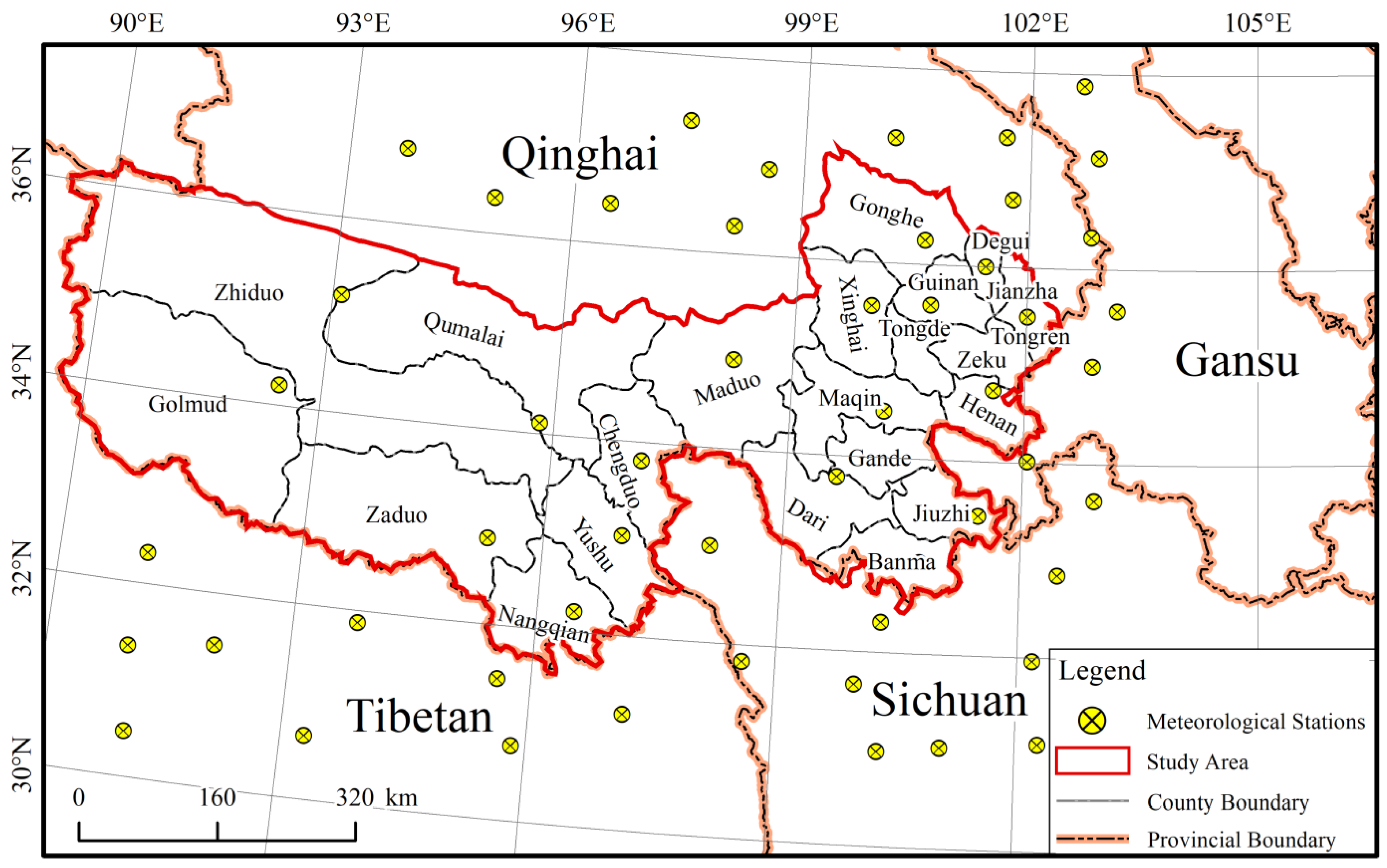
2.1. Overview of the Study Area

The Three-River headwaters region has a vast territory, steep terrain and extremely undulating topography, and its altitude shows a trend of rising gradually from southeast to northwest as a whole, with a range of 1960–6700 m and an average altitude of about 4400 m. The western region has the highest average altitude, and its landform is mainly glacier; the mid-west and northern regions have relatively flat terrains and large areas of marshes and characterized by extremely undulating topography, the southeast region belongs to the alpine and gorge zone and is dominated by an eroded middle mountain landform, river valley landform and lake basin landform [39]. The Three-River headwaters region has a plateau continental climate and is part of the Tibetan Plateau climate system. It has an average annual temperature of −5.7 to 7.8 °C, an annual precipitation of 262.2–772.8 mm and a trend of increasing from northwest to southeast [40]. The geographical location of the study area is shown in Figure 1.

2.2. Data Source and Preprocessing

2.2.1. Remote Sensing Data

This study obtained the MODIS/Terra MOD09A1 from the National Aeronautics and Space Administration (NASA). The MOD09A1 product was synthesized by the MODIS Level-2G product (MOD09GA), and each pixel contained the optimal observation over 8 days based on conditions such as high observation coverage, low viewing angle, no cloud or cloud shadow and aerosol load. The data was composed of 7 spectral bands with a spatial resolution of 500 m. The NDVI calculated by MOD09A1 in the sinusoidal projection mode was reused to calculate the phenological data. The calculation formula of the NDVI is shown in Formula (1).

$$NDVI=\frac{{\rho }_{nir}-{\rho }_{red}}{{\rho }_{nir}+{\rho }_{red}}$$

(1)

where ${\rho }_{red}$ and ${\rho }_{nir}$ are the MODIS red (620–670 nm) and near-infrared (841–876 nm) bands, respectively.

According to the geographical location of the Three-River headwaters region in the world, the h25v05 and h26v06 coordinates were selected, and the GLASS LAI data from 2001 to 2018 was obtained from the National Earth System Science Data Center (http://www.geodata.cn, accessed on 2 December 2021). There were 92 images every year, and a total of 1656 images were downloaded. The mode of sinusoidal projection was adopted for the downloaded data file, with a range of effective values of 0–1000 pixels. The water body was filled with 2000, and the invalid data was filled with 2500, with a scale coefficient of 0.01.

The GLASS LAI used in this study was calculated by using surface reflectance products (MOD09A1) on a global scale by the general regression neural network (GRNN) method [41]. Firstly, the “effective” Cyclope LAI was converted to the actual value using the aggregation index (Ω) by Formula (2):

$$LA{I}_{act}=LA{I}_{eff}/\Omega$$

(2)

Then, a weighted linear combination of MODIS and Cyclope LAI was established to obtain the optimal LAI estimated value. The MOD09A1 data was reprocessed to remove the cloud pollution, and the missing blank points were filled to obtain the spatial–temporal continuous and smooth data [42]. GRNN was trained using fusion LAI for each biota type and MOD09A1 data from the benchmark land multi-site analysis and product comparison site (BELMANIP).

2.2.2. Meteorological Data

Three meteorological data sets—namely, air temperature, precipitation and sunshine duration—were used in this study. The data was downloaded in text format from the CMA Meteorological Data Centre (http://data.cma.cn/, accessed on 15 February 2022) during the period from 1 January 2001 to 31 December 2018. A total of 53 meteorological stations were used, of which 18 were distributed within the study area and 35 were distributed around it. The locations of the meteorological stations are shown in Figure 2. In this study, interpolation of the air temperature and precipitation data was achieved by the method of partial thin plate smoothing spline (PTPS), while interpolation of the sunshine duration data in the study area was achieved by using the Kriging method with ArcGIS and obtained 500-m resolution images.

2.2.3. Elevation Data

The elevation data used in this study is SRTM3 (Shuttle Radar Topography Mission 3) V4.1 digital elevation model data, which was downloaded from Geospatial Data Cloud (http://www.gscloud.cn, accessed on 9 January 2022). The data has a spatial resolution of 90 m and is presented in GeoTIFF format, and its original coordinate system is GCS_WGS_1984. In this paper, the Digital Elevation Model (DEM) data in the study area was obtained by splicing, embedding, reprojection and clipping. Based on this, a 500-m spatial resolution grid was generated from remote sensing images through regional statistics, and grids were used to extract the corresponding regional topographic factors by using the space averaging method.

2.3. Study Methods

2.3.1. Extraction Methods of Vegetation Phenology

(1)

Time series reconstruction

Vegetation growth is affected by hydrothermal conditions. Due to high temperatures and abundant precipitation in the spring and summer, the LAI value shows an upward trend, while, in the autumn and winter, the LAI value shows a downward trend due to low temperatures and a lack of precipitation. There will be noise and mutation points in the actually obtained vegetation LAI remote sensing data due to the influence of different atmospheric conditions, sensors and aerosols [43]. A smooth mathematical function curve will be used to fit the time series containing noise so as to keep the integrity of the original data as much as possible under the premise of reducing the impact of the noise. In this study, the A-G fitting method was adopted to reconstruct the time series data. The A-G fitting method was proposed by Jӧnsson et al. for fitting a time series [22]. The fitting equation is shown in Formula (3):

$$f\left(t\right)=c_1+c_2·g\left(t;x_1,\cdots ,x_5\right)$$

(3)

where $f\left(t\right)$ is the fitted value at time $t$, $c_1$ and $c_2$ are used to determine the benchmark and amplitude of the fitting curve and $g\left(t;x_1,\cdots ,x_5\right)$ is the Gaussian function, as shown in Formula (4):

$$\left(t; x_1,\cdots ,x_5\right)=\left\{\begin{array}{c}exp\left[-{\left(\frac{t-x_1}{x_2}\right)}^{x_3}\right] t>x_1\\ exp\left[-{\left(\frac{x_1-t}{x_4}\right)}^{x_5}\right] t<x_1\end{array}\right.$$

(4)

where $x_1$ is the central point of the fitting window, $x_2$ and $x_3$ are used to determine the width and height of the fitting window on the right, respectively, and $x_4$ and $x_5$ are used to determine the width and height of the fitting window on the left, respectively.

(2)

Phenological extraction

Piao et al. proposed a method for extracting vegetation phenology, which has been widely used to study vegetation phonological changes on a large scale [44]. The calculation method is shown in Formula (5):

$$LA{I}_{ratio}\left(t\right)=\left[LAI\left(t+1\right)-LAI\left(t\right)\right]/LAI\left(t\right)$$

(5)

where $t$ refers to the time serial number corresponding to the pixel, and $LAI\left(t\right)$ is the GLASS LAI value corresponding to the pixel at time$t$. When $LA{I}_{ratio}\left(t\right)$ reaches the maximum value, the corresponding $t$ is the start of the growing season (SOS) of the vegetation; when $LA{I}_{ratio}\left(t\right)$ reaches the minimum value, the corresponding $t$ is the end of the growing season (EOS) of the vegetation. The difference between the EOS and SOS is the length of the growing season (LOS).

In other words, we first inferred the fastest change rates of the LAI corresponding to the vegetable SOS and EOS from the seasonal cycles of the LAI (March–May and August–October) from 2001 to 2018. Then, the onset dates of the vegetation of the SOS and EOS were determined based on the inferred rates and the LAI seasonal cycles, while the LOS of the vegetation was also determined. Finally, we acquired a total of 54 SOS, EOS and LOS images from 2001 to 2018 of the Three-River headwaters region (three SOS, EOS and LOS images per year, 18 years in total).

(3)

Evaluation index

In order to compare the effects of various fitting methods, frequently used methods such as the mean absolute error (MAE) and root mean square error (RMSE) and so on, are used to judge the magnitude of the sequence error before and after fitting. The MAE and RMSE have the advantages of keeping the numerical dimensions consistent with the original data dimensions, clear numerical meanings and convenient calculations. The RMSE is more sensitive to abnormal values [45]. The smaller the MAE and RMSE values are, the closer the fitting value is to the actual value, and the better the fitting effect is. The calculation formula is as follows:

$$MAE=\frac{1}{n}{{\displaystyle \sum }}_{i=1}^n\left|t_i-\widehat{t_i}\right|$$

(6)

$$RMSE=\sqrt{\frac{1}{n}{{\displaystyle \sum }}_{i=1}^n{\left(t_i-\widehat{t_i}\right)}^2}$$

(7)

where $n$ is the number of sample points, $t_i$ is the actual value of the sample point, and $\widehat{t_i}$ is the fitted value of the sample point.

2.3.2. Sen’s Trend Analysis

In nonparametric statistics, the Sen estimator is a method (simple linear regression) that firmly fits a line to a sampling point in the plane by choosing the median of the slopes of all the lines in a pair of points. Known also as the single median method, this estimator can be computed efficiently and is insensitive to outliers. It is much more accurate than the non-robust simple linear regression (least squares) for skewed and heteroscedastic data [46]. In this paper, the variation trends of the SOS, EOS and LOS of vegetation and the interannual variation trend of the meteorological data in the Three-River headwaters region were calculated through a Sen’s trend analysis, which is a simple and robust method for obtaining the variation trend of time series and can reduce the influence of abnormal values on the results [47]. The calculation method is shown in Formula (8):

$$Slope=median\left(\frac{x_j-x_i}{j-i}\right),1\le i<j\le n$$

(8)

where $i$ and $j$ represent the serial number value of the time series, $x_i$ and $x_j$ represent the SOS/EOS/LOS values of the vegetation corresponding to serial numbers I and j, respectively, and $n$ is the length of the time series. As this study was conducted from 2001 to 2018, $n$ was 18. In this formula, the slope between any two points needs to be calculated first, and there are $n\left(n-1\right)/2$ items in total; then, all slopes need to be sorted from smallest to largest. If $n$ is odd, item $\left(n+1\right)/2$ will be taken as the final result; if $n$ is even, the arithmetic mean of item $n/2$ and item $\left(n+2\right)/2$ will be taken as the final result. $Slope$ is the calculated trend value. If the $Slope$ is greater than 0, it means that this time series shows an increasing trend; if the $Slope$ is less than 0, it means that this time series shows a decreasing trend.

2.3.3. Mann–Kendall Test

The Mann–Kendall test method does not need to carry out a specific distribution test for the data series and can also participate in the trend test for extreme values. In a time series analysis, it is not necessary to specify whether a linear trend is present [48]. In this study, the significance of the results calculated by the Sen’s trend method was analyzed with the Mann–Kendall test [49], which is a nonparametric test method. The tested time series data do not need to be normally distributed or linear, and the results are robust. The calculation method of the Mann–Kendall statistic S is as follows.

$$S={\displaystyle \sum }_{i=1}^{n-1}{\displaystyle \sum }_{j=i+1}^{n}sgn\left(x_j-x_i\right)$$

(9)

$$sgn\left(x_j-x_i\right)=\left\{\begin{array}{c} 1, x_j>x_i\\ 0, x_j=x_i\\ -1, x_j<x_i\end{array}\right.$$

(10)

where the $sgn$ function is a symbol for taking the parameter values. Return to 1 if the parameter value is a positive number, return to −1 if the parameter value is a negative number and return to 0 if the parameter value is 0. If n is less than or equal to 10, its significance can be determined by looking up tables. When n is greater than 10, statistic S is approximately normally distributed, and standardized statistic Z needs to be constructed:

$$Z=\left\{\begin{array}{c}\frac{S-1}{\sqrt{var\left(S\right)}}, S>0\\ 0, S=0\\ \frac{S+1}{\sqrt{var\left(S\right)}}, S<0\end{array}\right.$$

(11)

$$var\left(S\right)=\frac{n\left(n-1\right)\left(2n+5\right)-{{\displaystyle \sum }}_{i=1}^m{c}_i\left(c_i-1\right)\left(2c_i+5\right)}{18}$$

(12)

where $var\left(S\right)$ is the variance of statistic S, $n$ is the number of points in the time series, $m$ is the number of repeated values in the time series and $c_i$ is the number of times of the $i$th repeated value. The null hypothesis is that the time series does not have a monotonous trend, while the alternative hypothesis is that the time series has a trend to change monotonously. The significance test level is set as $\alpha$; when $\left|Z\right|>Z_{1-\alpha }$ (standard normal variance), the null hypothesis is rejected, and the alternative hypothesis is accepted—that is, the time series has a monotonous trend. In this study, the significance level $\alpha$ was 0.05.

2.3.4. Partial Correlations Analysis

The Pearson correlation coefficient can be used to measure the degree of linear correlation between two time series, with a value range of −1 to 1. The greater the absolute value of the coefficient is, the stronger the linear correlation will be. When the value is in the range of −1 to 0, it indicates that there is a linear negative correlation between the two time series; when the value is 0, it indicates that there is no linear relationship between the two time series and when the value is in the range of 0 to 1, it indicates that there is a linear positive correlation between the two time series. Although the degree of correlation between the climate factor and phenological factor can be calculated by the Pearson correlation coefficient, vegetation phenology is also affected by the temperature, precipitation, sunshine duration and other factors simultaneously. In order to analyze the correlation between a single meteorological factor and vegetation phenology, a partial correlation analysis was used to eliminate the influence of other climate variables. The partial correlation coefficient is calculated as follows:

$$r_{x_{1}y·x_2{x}_3}=\frac{r_{x_{1}y·x_2}-r_{x_1{x}_3·x_2}·r_{x_{3}y·x_2}}{\sqrt{\left(1-r_{x_1{x}_3·x_2}^2\right)\left(1-r_{x_{3}y·x_2}^2\right)}}$$

(13)

$$r_{x_{1}y·x_2}=\frac{r_{x_{1}y}-r_{x_{1}y}·r_{x_{1}y}}{\sqrt{\left(1-r_{x_{1}y}^2\right)\left(1-r_{x_{2}y}^2\right)}}$$

(14)

$$r_{xy}={{\displaystyle \sum }}_{i=1}^n\frac{\left(x_i-\overline{x}\right)\left(y_i-\overline{y}\right)}{\sqrt{{{\displaystyle \sum }}_{i=1}^n{\left(x_i-\overline{x}\right)}^2}\sqrt{{{\displaystyle \sum }}_{i=1}^n{\left(y_i-\overline{y}\right)}^2}}$$

(15)

where $n$ is the number of points in the time series, $x_i$ and $y_i$ are the points in the time series of the meteorological factors and vegetation phenology and $\overline{x}$ and $\overline{y}$ are the mean values of the corresponding time series, respectively. $r_{xy}$ is the Pearson correlation coefficient between two time series, and $r_{x_{1}y·x_2}$ is the partial correlation coefficient between $x_1$ and $y$ after the control factor $x_2$ and also known as the first-order partial correlation coefficient. $r_{x_{1}y·x_2{x}_3}$ is the partial correlation coefficient between $x_1$ and $y$ after the control factors $x_2$ and $x_3$ and also known as the second-order partial correlation coefficient. In this study, $x_1$, $x_2$ and $x_3$ correspond to the air temperature, precipitation and sunshine duration, respectively, and $y$ corresponds to the SOS/EOS of the vegetation. For example, $r_{air temperature SOS·precipitation \mathrm{sunshine}}$ is the partial correlation coefficient between the air temperature and SOS of the vegetation after controlling the precipitation and sunshine duration factors. The significance of the partial correlation analysis results can be calculated by the t-test method:

$$t=\frac{r_{x_{1}y·x_2{x}_3}}{\sqrt{1-r_{x_{1}y·x_2{x}_3}^2}}\sqrt{n-q-1}$$

(16)

where $n$ is the number of points in the time series. In this study, n was 18; $q$ is the number of factors, and there are 3 factors in this paper; $r_{x_{1}y·x_2{x}_3}$ is the second-factor partial correlation coefficient and $t$ obeys the t-distribution of $n-q-1$ degrees of freedom. The significance value of the partial correlation coefficient can be determined by querying the $t$ distribution table.

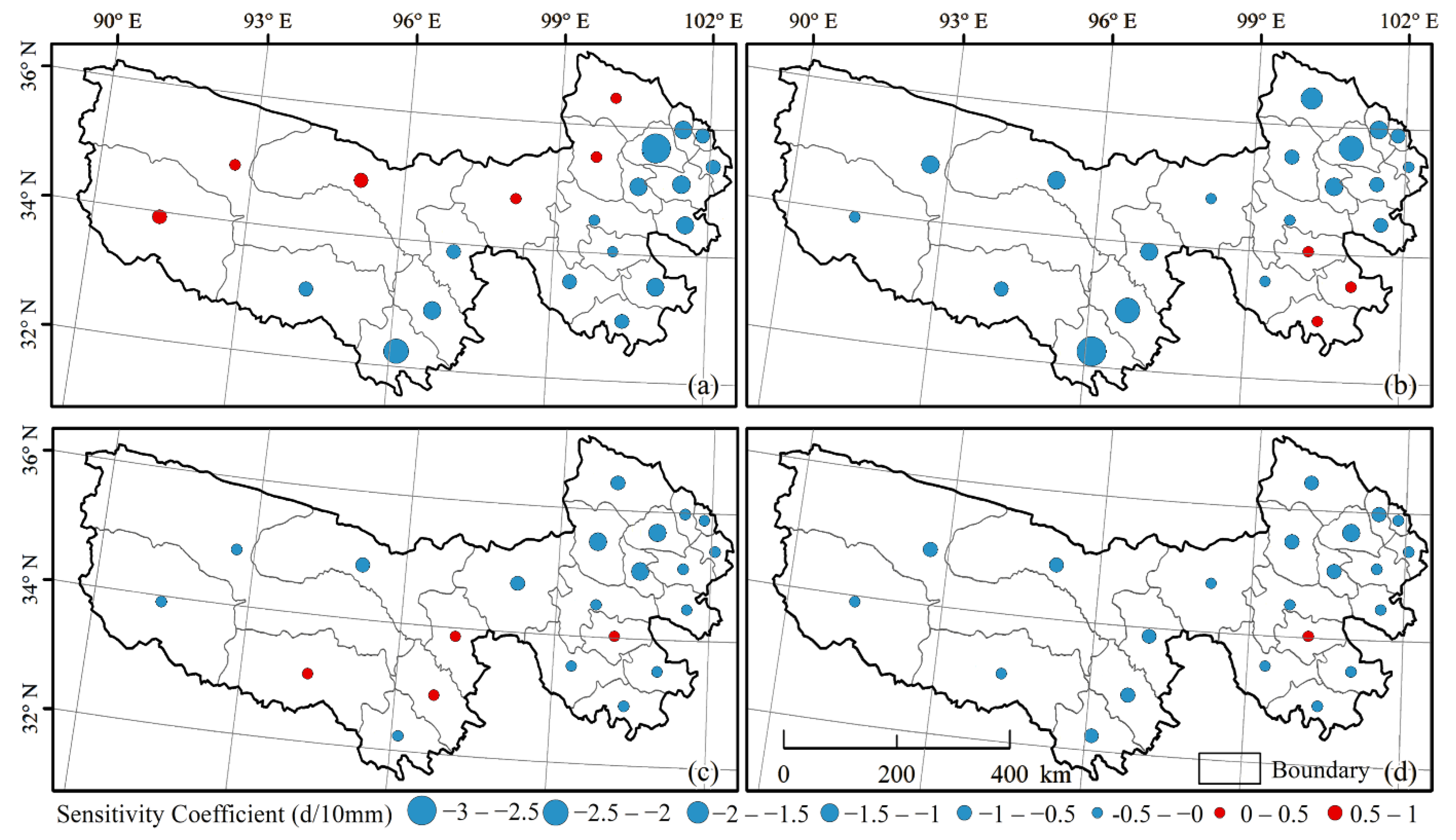
2.3.5. Sensitivity Analysis

There is spatial heterogeneity in the sensitivity of different meteorological factors during vegetation phenology and similarly for the same meteorological factors in different months [50]. The change of phenology depends on the influence of many factors, and it is difficult to distinguish the primary and secondary ones. In this study, multiple factors were used as independent variables to explain the changes in phenology.

In order to measure the degree of such sensitivity, this paper calculated the sensitivity of the SOS/EOS of the vegetation to the three meteorological factors (temperature, precipitation and sunshine duration) in the Three-River headwaters region through multiple linear regressions. The calculation method is shown in Formula (17):

$$y=b_0+b_1{x}_1+b_2{x}_2+b_3{x}_3$$

(17)

where y is the SOS/EOS of vegetation; $x_1$, $x_2$ and $x_3$ represent the temperature factor, precipitation factor and sunshine duration factor, respectively; $b_1$, $b_2$ and $b_3$ are the coefficients of sensitivity of the SOS/EOS of the vegetation to the temperature, precipitation and sunshine duration, respectively, and $b_0$ is a constant term. The absolute value of the sensitivity coefficient reflects the degree of sensitivity of the SOS/EOS of the vegetation and the meteorological factors. When the sign of the sensitivity coefficient is positive, it means that the corresponding factor plays a role in delaying the SOS/EOS of the vegetation; when the sign of the sensitivity coefficient is negative, it means that the corresponding meteorological factor plays a role in advancing the SOS/EOS of the vegetation.

3. Results

3.1. Extraction Results of Phenological Data

This paper extracted the three types of phenological data of the vegetation (namely, the SOS, EOS and LOS) by using the maximum slope method. The SOS, EOS and LOS data of the vegetation extracted year by year in the Three-River headwaters region was used pixel by pixel to calculate the multi-year mean value so as to get the spatial distribution of the SOS, EOS and LOS of the vegetation in the Three-River headwaters region, as shown in Figure 3.

Figure 3a shows the spatial distribution of the multi-year mean values of the vegetation SOS in the Three-River headwaters region from 2001 to 2018. From the analysis of Figure 3a, it can be seen that, in the Three-River headwaters region, the SOS of the vegetation is relatively early in the east, with a trend of increasingly later as it moves west, with the northwest the latest. The SOS of the vegetation in the Three-River headwaters region is mainly concentrated in the period from the 125th day of the year (early May) to the 150th day (late May), accounting for 81.11% of the vegetation area in the Three-River headwaters region. It can be seen from Figure 3c that the EOS of the vegetation in the Three-River headwaters region shows a decreasing trend from southeast to northwest, on the whole. The EOS of the vegetation in most of the study area is distributed in the period from the 269th day to the 284th day (late September to mid-October), accounting for 92.94%. In the Three-River headwaters region, the spatial distribution (see Figure 3e) of the LOS of the vegetation is basically consistent with that of the former two and still shows a decreasing trend from southeast to northwest. The length of the growing season in the Three-River headwaters region is mostly concentrated in the period of 115–165 days (3.8–5.5 months), accounting for 96.99%.

Figure 3b shows that there are great differences in the SOS of vegetation among the administrative regions of the Three-River headwaters region. In Jainca and Tongren Counties, the proportion of pixels of the SOS (earlier than the 125th day) of the vegetation is the highest, reaching up to 50%, and the corresponding SOS of the vegetation is the earliest, which are the 123rd day and the 124th day, respectively. In Zhiduo and Maduo Counties, the SOS of vegetation is the latest, which are the 148th day and the 146th day, respectively. It is worth noting that the proportion of pixels of the SOS (earlier than the 140th day) of the vegetation in the Mongolian Autonomous County of Henan reaches up to 99%, and the corresponding SOS of the vegetation is the 127th day. It can be seen from Figure 3d that the EOS of the vegetation is earlier (about the 272nd day) in Maduo, Qumarleb, Golmud and Zhiduo Counties but the latest (the 280th day) in the Mongolian Autonomous County of Henan. Figure 3f indicates that there are great differences in the LOS of the vegetation among the administrative regions of the Three-River headwaters region, with a range of 29 days. The LOS of the vegetation in the Mongolian Autonomous County of Henan is the longest, reaching 153 days, and the proportion of pixels of the LOS of the vegetation (longer than 135 days) is about 90%; the LOS of the vegetation in Zhiduo County is the shortest, reaching only 124 days, and the proportion of pixels of the LOS of the vegetation (shorter than 125 days) is about 93%.

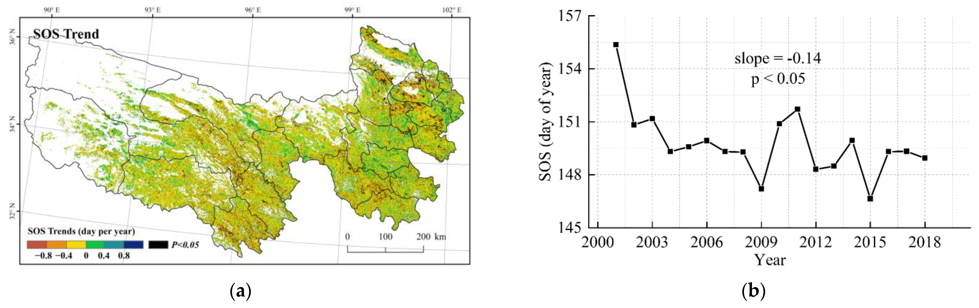
3.2. Temporal and Spatial Variation Trend of Vegetation Phenology

The SOS, EOS and LOS data of the vegetation obtained for many years was used pixel by pixel for the Sen’s trend analysis to get a variation trend of the vegetation phenological parameters, and the MK test was conducted to test the significance of the trend so as to obtain the spatial distributions of the variation trends of the SOS, EOS and LOS of the vegetation in the Three-River headwaters region, as shown in Figure 4 and

Table 1. Statistics of the variation trend of the SOS, EOS and LOS of the vegetation in the Three-River headwaters region from 2001 to 2018.

	Interannual Rate of Variation Classification (d/a)	Area Proportion (%)	Min of Interannual Variation Rate (d/a)	Max of Interannual Variation Rate (d/a)
SOS	<−0.8	7.71	−5.35	9.70
	−0.8–−0.4	19.77
	−0.4–0	47.84
	0–0.4	17.5
	0.4–0.8	5.63
	>0.8	1.55
EOS	<−0.6	2.05	−5.52	8.33
	−0.6–−0.3	9.71
	−0.3–0	31.9
	0–0.3	39.76
	0.3–0.6	13.98
	>0.6	2.60
LOS	<−1.2	1.23	−6.00	10.33
	−1.2–−0.6	5.46
	−0.6–0	33.72
	0–0.6	37.00
	0.6–1.2	17.95
	>1.2	4.64

d/a: day/year.

.

The spatial distribution and trend statistics of the interannual variation trend of the SOS of the vegetation in the Three-River headwaters region from 2001 to 2018 are shown in Figure 4a and Table 1. In the last 18 years, the SOS of the vegetation in the Three-River headwaters region varied in the range of −5.35–9.70 d/a (Table 1) and showed an advanced trend on the whole. A change in the SOS of the vegetation of −0.4 to 0 days/year was most common (47.84%, Table 1), which meant that there was a significant trend (p < 0.05, MK significance test) toward an earlier SOS between 2001 and 2018 (Figure 4b). However, for the EOS of the vegetation, the most common variations were in the slightly negative (−0.4 to 0) and slightly positive (0 to 0.4) days/year classes, consistent with no significant change in the EOS in the 2001–2018 period (Figure 4d). Similarly, for the LOS of the vegetation, the most common variations were in the slightly negative (−0.6 to 0) and slightly positive (0 to 0.6) days/year classes, consistent with no significant change in the LOS in the 2001–2018 period (Figure 4f).

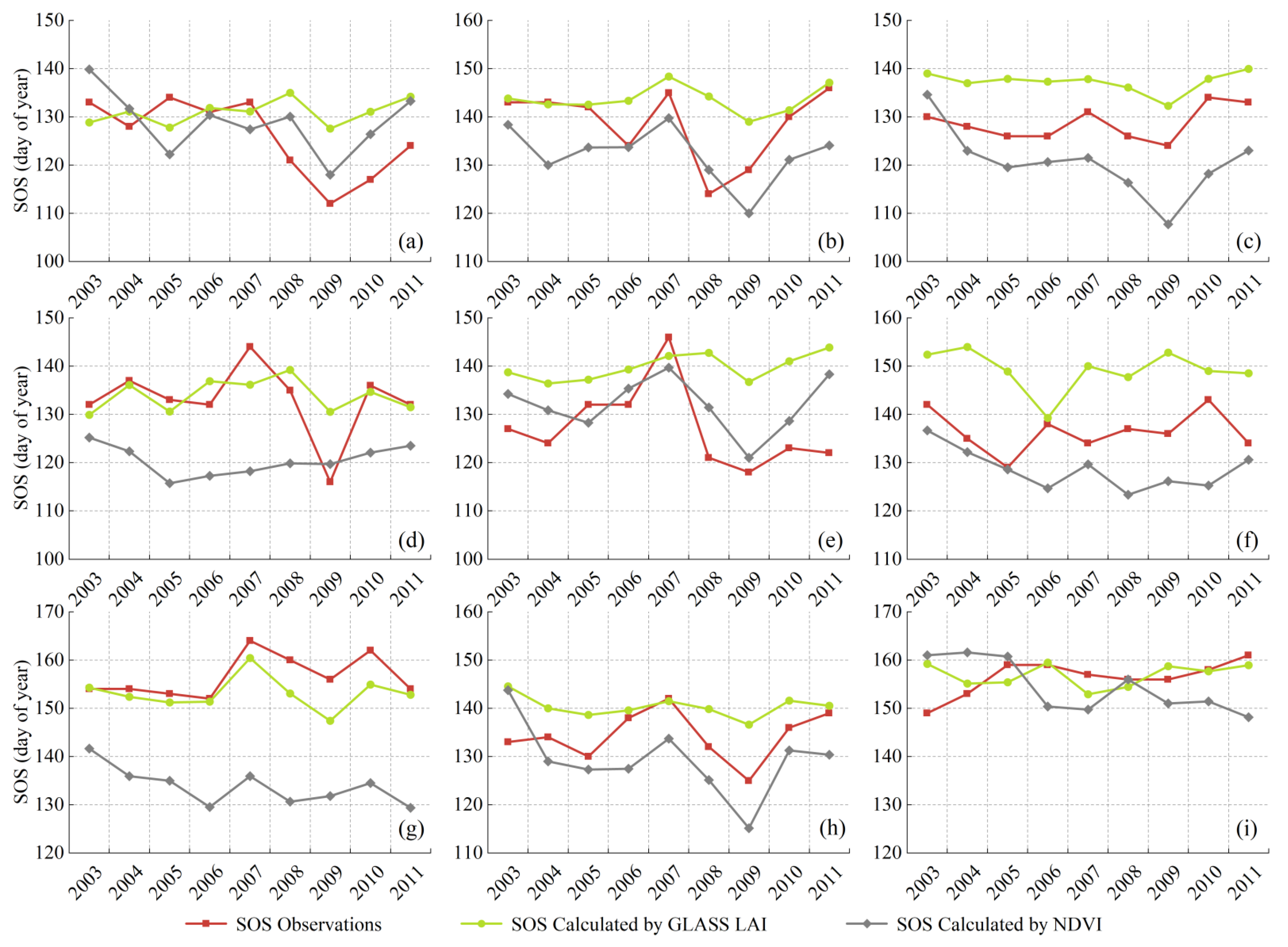
3.3. Precision Analysis

Based on the phenological observation data of nine meteorological stations, including Banma, Gande, Mongolian Autonomous County of Henan, Jiuzhi, Maqin, Nangqian, Qingshuihe, Zeku and Tuotuohe, the SOS of the vegetation calculated by using remote sensing data was verified in this paper. The phenological data observed at the station was generated by averaging the phenological values of the meteorological station within a radius of 5 km [51]. Figure 5 shows the comparisons among the phenological observation data, phenological data calculated based on the GLASS LAI and phenological data calculated based on the NDVI during the analysis period and a high level of consistency among the three types of data at most stations. Among the nine verified stations, except for Banma, Maqin and Tuotuohe, the SOS of the vegetation based on the GLASS LAI was better than that based on the NDVI in the remaining stations. The SOS of the vegetation based on the GLASS LAI and the SOS of the vegetation observed had a MAE of 7.6 d and a RMSE of 8.4 d. Considering that the temporal resolution of the GLASS LAI remote sensing data was 8 days, the SOS results of the vegetation calculated based on this data had a higher precision. The SOS of the vegetation based on the NDVI and the SOS of the vegetation observed had a MAE of 9.9 d and a RMSE of 10.9 d. In general, the SOS calculated based on the GLASS LAI, the SOS calculated based on the NDVI and the SOS observed can maintain consistency, indicating that the methods of phenology extraction in this paper were effective and reliable. According to the mean absolute error and root mean square error, the SOS results calculated based on the GLASS LAI were slightly better than those calculated based on the NDVI, as shown in

Table 2. Error comparison of the SOS data of the vegetation in the Three-River headwaters region.

Data Set	Error Index	Station
		Banma	Gande	Mongolian Autonomous County of Henan	Jiuzhi	Maqin	Nangqian	Qingshuihe	Zeku	Tuotuohe
LAI	RMSE	12.9	8.3	8.9	6.0	17.6	14.0	4.6	7.3	4.1
	MAE	10.3	5.2	8.6	4.3	15.8	12.7	3.5	6.1	3.0
NDVI	RMSE	7.6	8.3	10.1	14.7	8.0	9.7	23.4	7.9	8.0
	MAE	6.9	7.4	9.2	13.4	7.0	7.9	22.7	7.5	7.0

.

3.4. Relationship between Vegetation Phenology and Topography

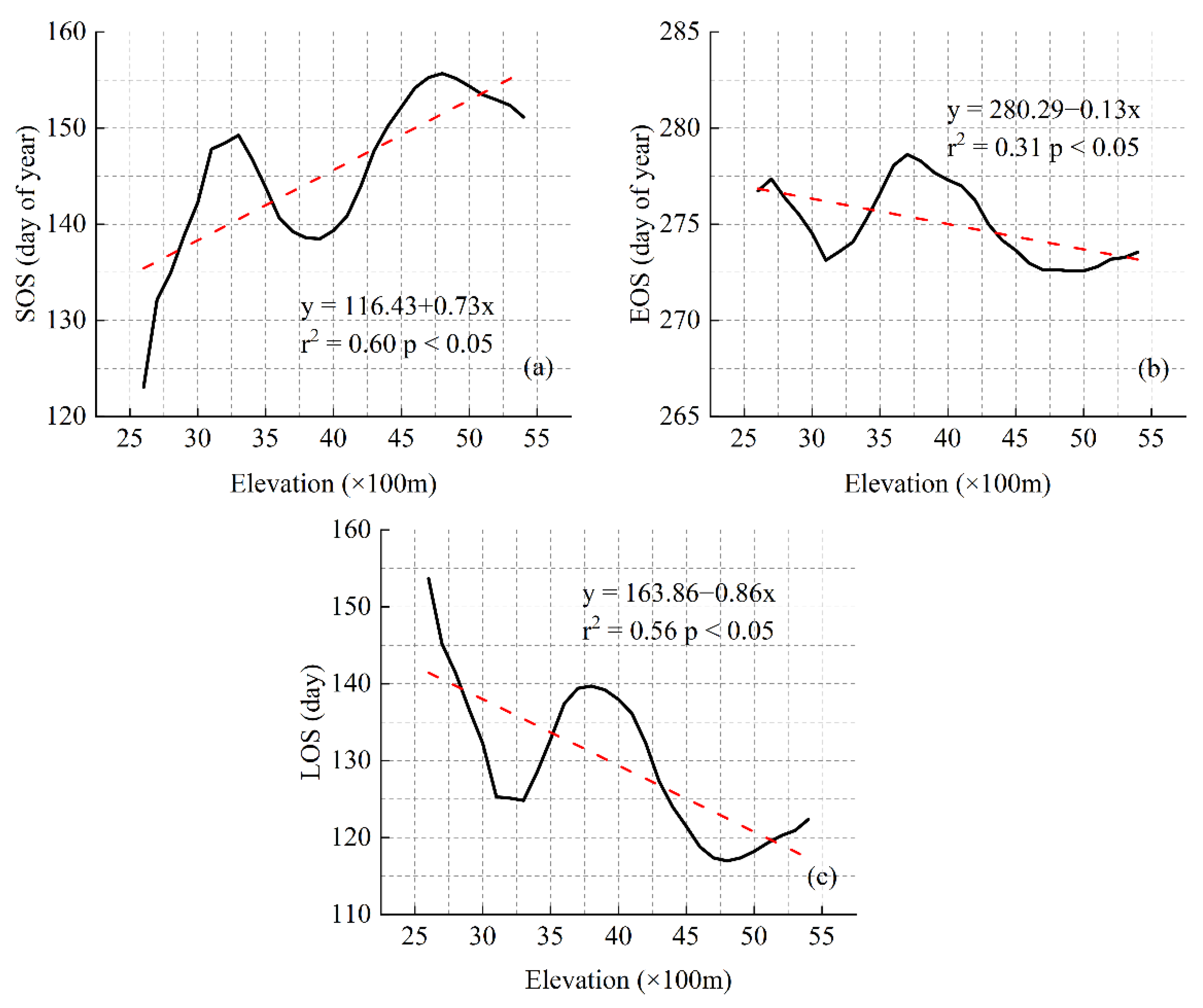
3.4.1. Relationship between Vegetation Phenology and Altitude

The Three-River headwaters region is characterized by complex terrain, extremely undulating topography and vertical zonal differentiation of the vegetation phenology. The elevation data were classified in 100-m intervals, and the change of the phenological index with the elevation was calculated by a unary linear regression model. It can be seen from Figure 6 that the SOS of the vegetation is delayed with an increase in the altitude, but the EOS is only slightly advanced, so the significant decrease in the LOS is largely caused by changes in the SOS.

Figure 6 demonstrates the relationship between the SOS, EOS and LOS of the vegetation changing and altitude in the Three-River headwaters region. It can be seen from Figure 6a that the SOS of the vegetation tends to be delayed with the increase of the altitude as a whole. The SOS of the vegetation will be delayed by 0.73 days for every 100-m increase in altitude. In addition, the curve has three extreme points, and their corresponding altitudes are 3300 m, 3900 m and 4800 m, respectively. The SOS of the vegetation will be delayed by 3.65 days for every 100-m increase in altitude in the altitude range of 2600–3300 m, be advanced by 1.90 days for every 100-m increase in altitude in the altitude range of 3300–3900 m, be delayed by 2.18 days for every 100-m increase in altitude in the altitude range of 3900–4800 m and be advanced by 0.74 days for every 100-m increase in altitude in the altitude range of 4800–5400 m.

Figure 6b demonstrates that the EOS of the vegetation tends to be advanced with the increase of the altitude as a whole. The EOS of the vegetation will be delayed by 0.13 days for every 100-m increase in the altitude. In addition, the curve has three extreme points, and their corresponding altitudes are 3100 m, 3700 m and 4700 m, respectively. The EOS of the vegetation will be advanced by 0.78 days for every 100-m increase in altitude in the altitude range of 2600–3100 m, be delayed by 1.00 day for every 100-m increase in altitude in the altitude range of 3100–3700 m, be advanced by 0.65 days for every 100-m increase in altitude in the altitude range of 3700–4700 m and be delayed by 0.14 days for every 100-m increase in altitude in the altitude range of 4700–5400 m.

Figure 6c demonstrates the variation of the LOS of the vegetation with the altitude in the Three-River headwaters region and also shows that the LOS of the vegetation tends to be shortened with the increase of the altitude. The LOS of the vegetation is shortened by 0.86 days for every 100-m increase in the altitude. In addition, the curve has three extreme points, and their corresponding altitudes are 3300 m, 3800 m and 4800 m, respectively. The LOS of the vegetation is shortened by 4.22 days for every 100-m increase in altitude in the altitude range of 2600–3300 m, be prolonged by 3.19 days for every 100-m increase in altitude in the altitude range of 3300–3800, be shortened by 2.69 days for every 100-m increase in altitude in the altitude range of 3800–4800 m and be prolonged by 0.91 days for every 100-m increase in altitude in the altitude range of 4800–5400 m.

From a comprehensive perspective, Figure 6 demonstrates that the SOS of the vegetation is delayed with the increase of the altitude, the EOS of the vegetation is advanced with the increase of the altitude and the LOS of the vegetation is shortened with the increase of the altitude. The variation characteristics of the LOS of the vegetation are largely caused by the variation of the SOS of the vegetation.

3.4.2. Relationship between Vegetation Phenology and Slope

In the Three-River headwaters region, the terrain is steep in the southeast but relatively flat in the northwest. In order to analyze the relationship between the vegetation phenology changing and the slope, the slope data was graded at 0.5° intervals, and the information of the SOS, EOS and LOS of the classified slope counted. When the slope was greater than 28°, the number of corresponding pixels was too small, so it was not analyzed.

Figure 7 demonstrates the relationship between the SOS, EOS and LOS of the vegetation and slope in the Three-River headwaters region. Vegetation phenology has a strong correlation with the slope. As the slope increases, the SOS of the vegetation is advanced (Figure 7a), the EOS of the vegetation is delayed (Figure 7b) and the LOS of the vegetation is prolonged (Figure 7c). For every 1° increase in the slope, the SOS of the vegetation is advanced by 0.42 days (Figure 7a), the LOS of the vegetation is delayed by 0.05 days (Figure 7b) and the LOS of the vegetation will be delayed by 0.42 days (Figure 7c).

3.5. Relationship between Vegetation Phenology and Meteorological Factors

If the interannual variation of the cumulative precipitation and air temperature correlate positively with the vegetation phenological characteristics—that is, the increase of the climatic factor values can change in the vegetation SOS and EOS—the LOS vegetation will be further changed, and the correlation coefficients need to be compared to determine whether such a change of the LOS of the vegetation is caused by the SOS or the EOS of the vegetation. Studies have shown that the land surface phenological models of vegetation often have a time lag response to climate factors. The Three-River headwaters region is located in the hinterlands of the Qinghai–Tibet Plateau, with high altitudes and variable climatic factors. In terms of time, the phenological pattern of the vegetation in different areas may have a lag and cumulative response to different climatic factors.

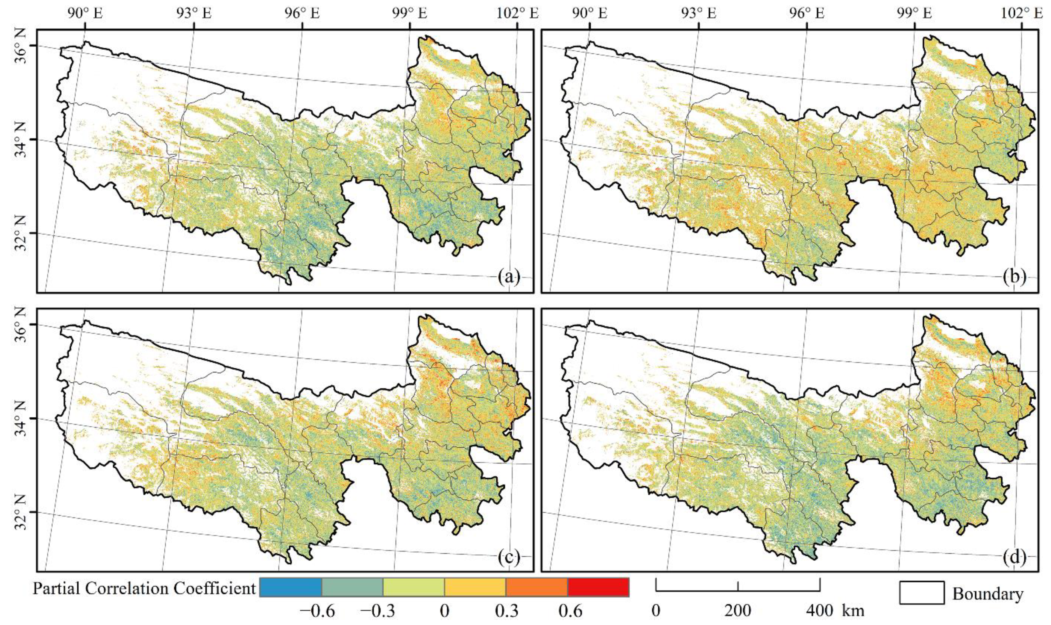
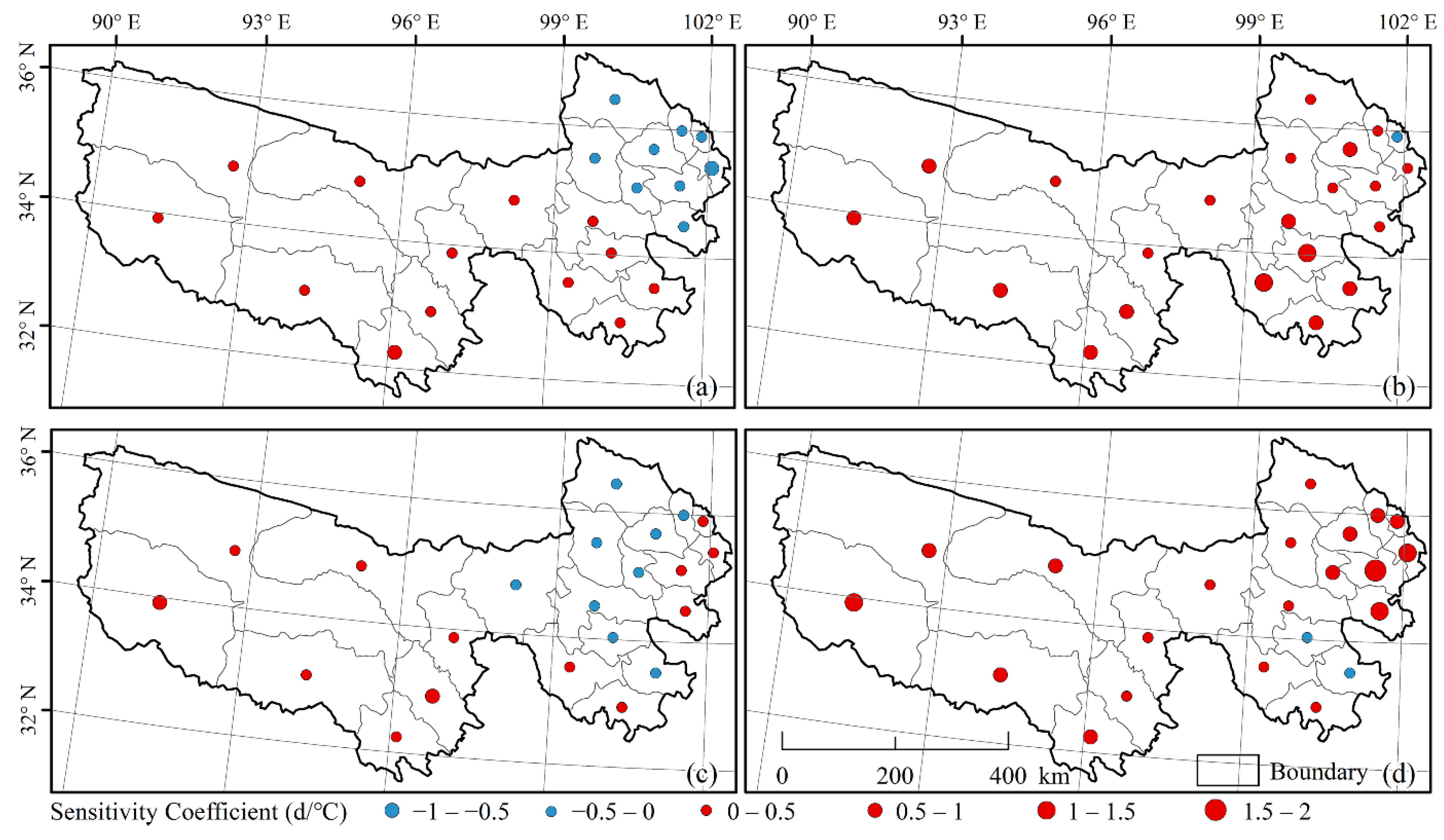
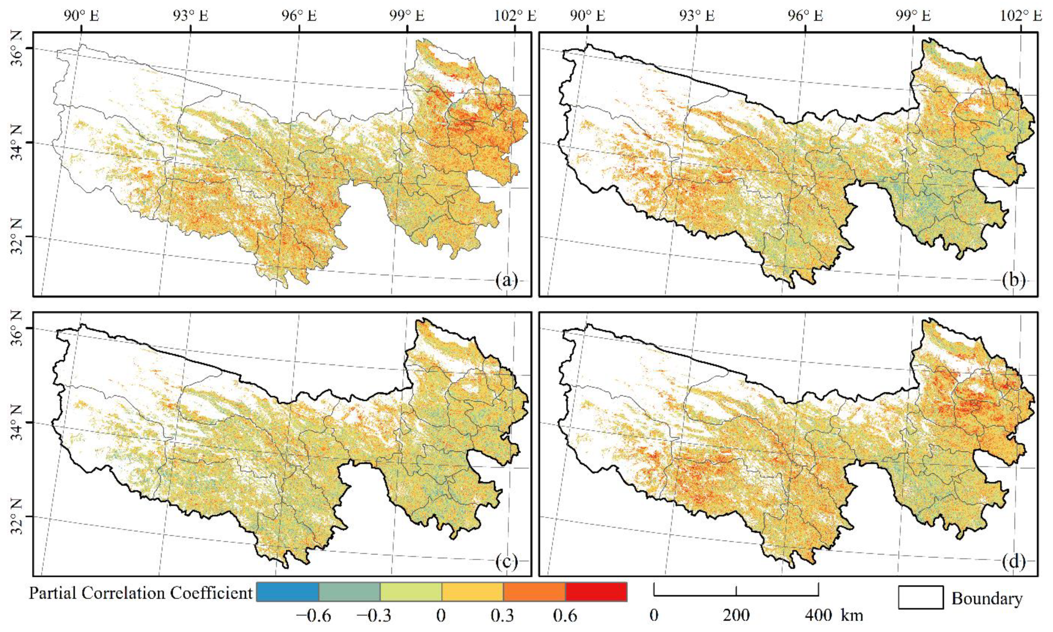
3.5.1. Relationship between SOS of Vegetation and Meteorological Factors

In this study, the average temperature, cumulative precipitation and cumulative sunshine duration of March, April, May and March–May were selected to calculate the partial correlation coefficients between the SOS of the vegetation and the climate factors in different time periods, so as to study the response relationship between the SOS of the vegetation and the climate. The partial correlation coefficient has a value range of −1 to 1. The closer the value is to 1, the stronger the positive correlation is; the closer the value is to −1, the stronger the negative correlation is. Meanwhile, the sensitivity of the SOS of the vegetation to different meteorological factors was calculated by multiple linear regressions, as shown in Figure 8, Figure 9, Figure 10, Figure 11, Figure 12 and Figure 13 and

Table 3. Statistics on the correlation between the SOS of the vegetation and meteorological factors in different time periods (%).

Meteorological Factor	Positive Correlation	Significant Positive Correlation	Negative Correlation	Significant Negative Correlation
$T_3$	26.58	0.65	73.42	8.92
$T_4$	42.00	1.72	58.00	4.10
$T_5$	32.85	1.23	67.15	6.39
$T_{3–5}$	27.45	0.90	72.45	9.07
$P_3$	42.10	1.72	57.90	4.10
$P_4$	38.64	1.67	62.23	5.64
$P_5$	41.46	1.48	58.54	4.13
$P_{3–5}$	34.11	1.29	65.89	6.71
$S_3$	49.16	2.24	50.84	2.55
$S_4$	38.64	1.33	61.36	4.68
$S_5$	52.81	2.50	47.19	1.61
$S_{3–5}$	43.97	1.55	56.03	3.01

$T_3$ is the average temperature for March, $T_4$ is the average temperature for April, $T_5$ is the average temperature for May and $T_{3–5}$ is the average temperature for March–May; $P_3$ is the cumulative precipitation for March, $P_4$ is the cumulative precipitation for April, $P_5$ is the cumulative precipitation for May and $P_{3–5}$ is the cumulative precipitation for March–May and $S_3$ is the cumulative sunshine duration for March, $S_4$ is the cumulative sunshine duration for April, $S_5$ is the cumulative sunshine duration for May and $S_{3–5}$ is the cumulative sunshine duration for March–May.

.

Figure 13 shows the spatial distribution of the sensitivity coefficients between the SOS of the vegetation and cumulative sunshine duration in March, April, May and March–May in the Three-River headwaters region. There is a great difference in the spatial distribution of the sensitivity coefficients between the SOS of the vegetation and cumulative sunshine duration. The SOS of the vegetation was advanced by 0.02 d for every 10-h increase in the cumulative sunshine duration in March. In the study area, the sensitivity coefficients between the SOS of the vegetation and cumulative sunshine duration in March were positive in 10 administrative regions distributed in the northeast, southwest and northwest of the study area. In particular, the sensitivity coefficient of Gonghe County was 0.67 d/10 h, and the corresponding sensitivity coefficients of the remaining 12 administrative regions were in the range of −0.5–0 d/10 h. In most areas of the study area, the sensitivity coefficients between the SOS of the vegetation and cumulative sunshine duration in April were negative (the SOS of the vegetation was advanced by 0.42 d for every 10-h increase in the cumulative sunshine duration in April), especially in Nangqian County, where the sensitivity coefficient was −0.93 d/10 mm; in the study area, the sensitivity coefficients between the SOS of the vegetation and cumulative precipitation in May were in the range of −0.5–0.5 d/10 mm. The corresponding sensitivity coefficients in the western part of the study area were basically positive, while those in the eastern part were basically negative. The SOS of the vegetation was delayed by 0.09 d for every 10-h increase in the cumulative sunshine duration in May. Compared with the other months, the sensitivity coefficients between the SOS of the vegetation and cumulative sunshine duration in March–May were in the range of −0.5–0.5 d/10 h. The corresponding sensitivity coefficients of the other administrative regions, except Gonghe County, Xinghai County and the Mongolian Autonomous County of Henan, were all negative. The SOS of the vegetation was advanced by 0.10 d for every 10-h increase in the cumulative sunshine duration in March–May.

The results of the partial correlation analysis between the SOS of the vegetation and meteorological factors in the Three-River headwaters region showed that, among all the air temperature factors, the SOS of the vegetation has the strongest correlation with the air temperature in March–May in the Three-River headwaters region (Figure 9d). The proportion of negatively correlated pixels is 72.45%, while the proportion of significantly negatively correlated (p < 0.05) pixels is 9.07% (Table 3: T_3–5). The SOS of the vegetation is advanced by 1.97 d for every 1 °C increase in the air temperature in March–May. Among all the precipitation factors, the SOS of the vegetation has the strongest correlation with precipitation in March–May in the Three-River headwaters region (Figure 11d). The proportion of negatively correlated pixels is 65.89%, while the proportion of significantly negatively correlated (p < 0.05) pixels is 6.71% (Table 3: P_3–5). The SOS of the vegetation is advanced by 0.49 d for every 10-mm increase in the precipitation in March–May. Among all the sunshine duration factors, the SOS of the vegetation has strongest correlation with the sunshine duration in April in the Three-River headwaters region (Figure 13a). The proportion of negatively correlated pixels is 61.36%, while the proportion of significantly negatively correlated (p < 0.05) pixels is 4.68% (Table 3: S₄). The SOS of the vegetation is advanced by 0.42 d for every 10-h increase in the sunshine duration in April. The SOS of the vegetation is mainly affected by the air temperature in March–May.

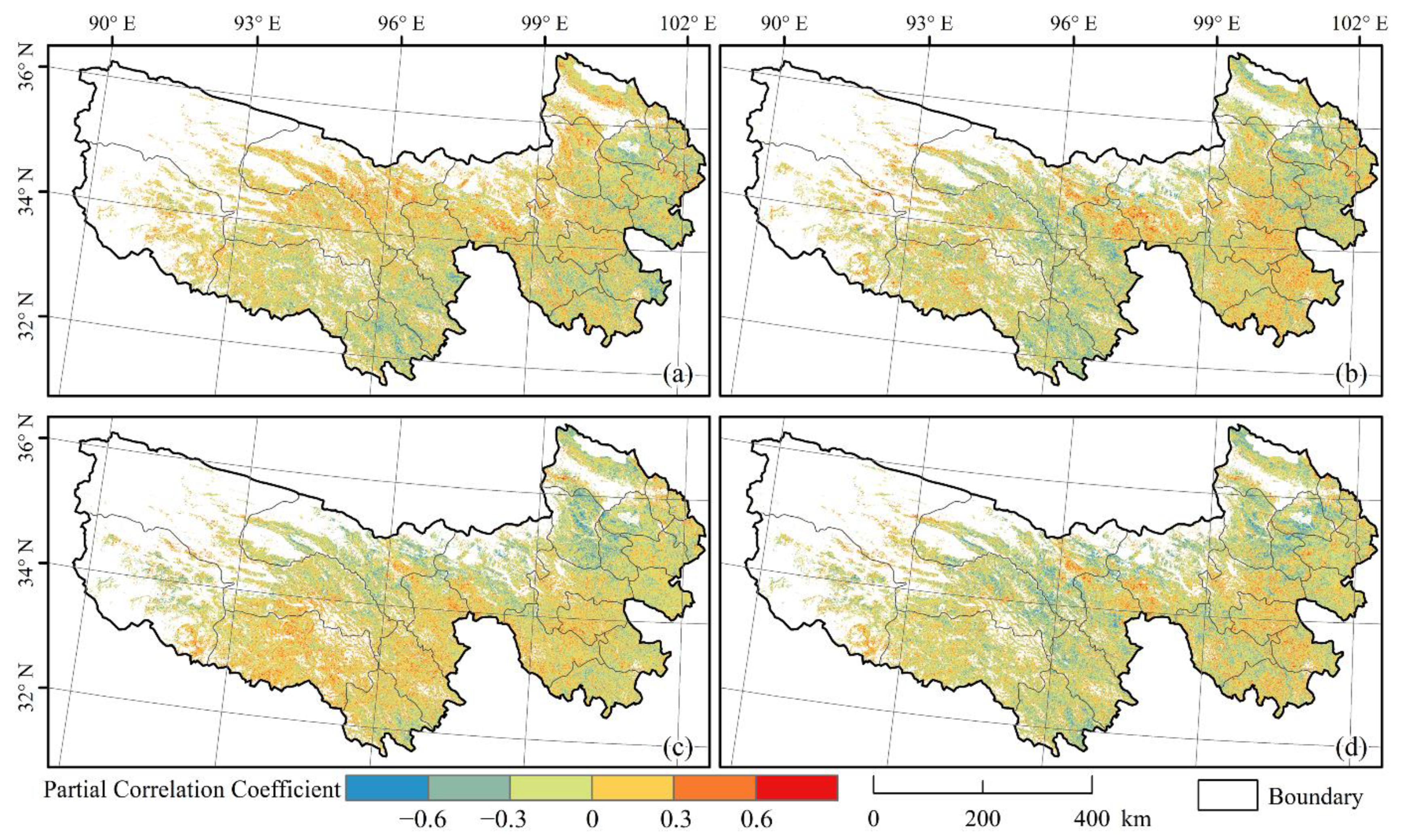
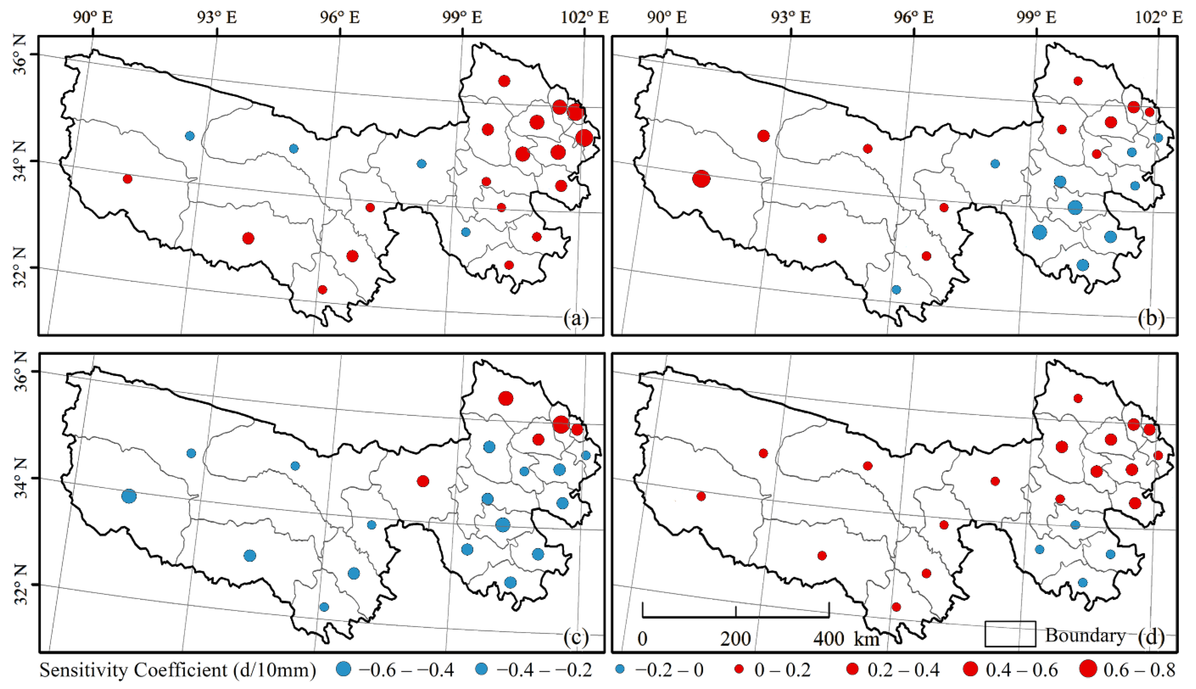
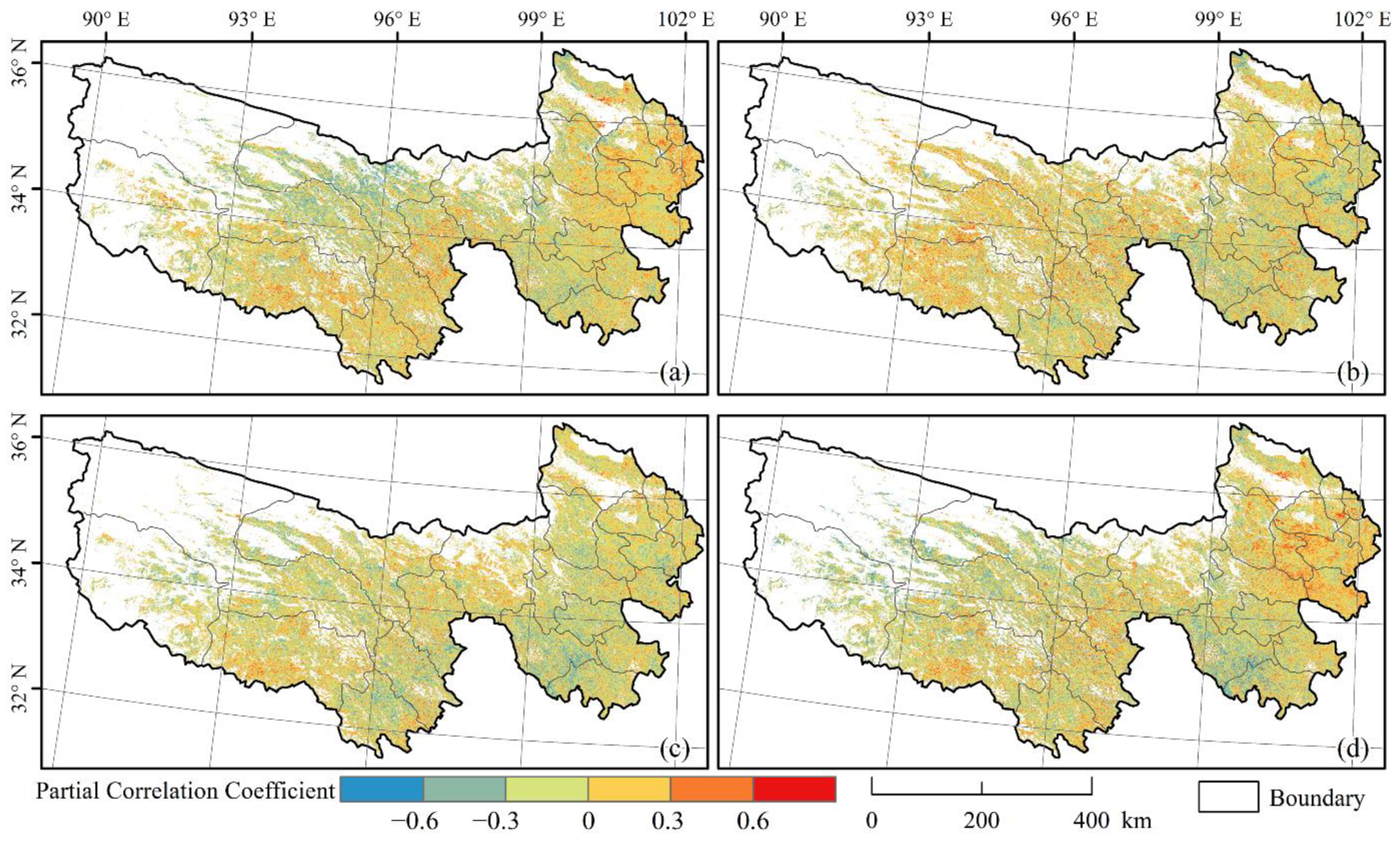
3.5.2. Relationship between EOS of Vegetation and Meteorological Factors

Considering the lag and cumulative response to the meteorological factors, this study selected the average temperature, cumulative precipitation and cumulative sunshine duration of August, September, October and August–October to calculate the partial correlation coefficients between the EOS of the vegetation and the meteorological factors so as to study the response relationship between the EOS of the vegetation and the autumn climate and calculate the sensitivity of autumn phenology to different climatic data, as shown in Figure 14, Figure 15, Figure 16, Figure 17, Figure 18 and Figure 19 and

Table 4. Statistics on the correlation between the EOS of the vegetation and meteorological factors in different time periods in the Three-River headwaters region (%).

Meteorological Factor	Positive Correlation	Significant Positive Correlation	Negative Correlation	Significant Negative Correlation
$T_8$	56.86	3.58	43.14	1.78
$T_9$	62.19	5.09	37.81	1.61
$T_{10}$	56.55	3.68	43.45	2.09
$T_{8–10}$	60.25	3.85	39.75	1.22
$P_8$	58.67	5.29	41.33	2.01
$P_9$	50.19	3.21	49.81	3.23
$P_{10}$	44.69	1.69	55.31	3.45
$P_{8–10}$	58.55	5.55	41.45	1.94
$S_8$	42.50	2.25	57.50	5.22
$S_9$	45.60	3.18	54.40	4.16
$S_{10}$	37.50	1.53	62.50	5.23
$S_{8–10}$	41.54	3.04	58.46	6.33

$T_8$ is the average temperature for August, $T_9$ is the average temperature for September, $T_{10}$ is the average temperature for October and $T_{8–10}$ is the average temperature for August–October; $P_8$ is the cumulative precipitation for August, $P_9$ is the cumulative precipitation for September, $P_{10}$ is the cumulative precipitation for October and $P_{8–10}$ is the cumulative precipitation for August–October and $S_8$ is the cumulative sunshine duration for August, $S_9$ is the cumulative sunshine duration for September, $S_{10}$ is the cumulative sunshine duration for October and $S_{8–10}$ is the cumulative sunshine duration for August–October.

.

The results of the partial correlation analysis between the EOS of the vegetation and meteorological factors in the Three-River headwaters region showed that, among all the air temperature factors, the EOS of the vegetation has the strongest correlation with the air temperature in September in the Three-River headwaters region (Figure 15b). The proportion of positively correlated pixels is 62.19%, while the proportion of significantly positively correlated (p < 0.05) pixels is 5.09% (Table 4: T₉). The EOS of the vegetation is delayed by 0.55 d for every 1 °C increase in the air temperature in September. Among all the precipitation factors, the EOS of the vegetation has the strongest correlation with precipitation in August–October in the Three-River headwaters region (Figure 17d). The proportion of positively correlated pixels is 58.55%, while the proportion of significantly positively correlated (p < 0.05) pixels is 5.55% (Table 4: P_8–10). The EOS of the vegetation is delayed by 0.10 d for every 10-mm increase in precipitation in August–October. With the sunshine duration, the EOS of the vegetation had the strongest correlation with the sunshine duration in October (Figure 19c). The proportion of the negatively correlated pixels is 62.5%, while 5.23% are significantly negatively correlated (Table 4: S₁₀). The EOS of the vegetation advanced by 0.26 d for every 10-h increase in the sunshine duration in October, the month that the sunshine duration mainly restricted the EOS.

4. Discussion

4.1. Comparative Analysis of Phenological Research Methods

As the Three-River headwaters region is located in the hinterlands of the Qinghai–Tibet Plateau, which is the highest and largest physical geographical unit on the Earth, previous researchers have made rich achievements in this region [52,53,54].

Table 5. Comparisons between this study and previous studies.

Study Periods	Data Sources	SOS of Vegetation (DOY)	EOS of Vegetation (DOY)	LOS of Vegetation (Day)	References
1999–2013	SPOT-VGT NDVI (1 km)	130–150	——	——	Liu et al. [52]
2000–2014	MOD09Q1 NDVI (250 m)	125–155	280–290	130–160	Liu [53]
2001–2018	MOD13A1 NDVI (500 m)	125–145	268–277	——	Sun [54]
2001–2018	GLASS LAI (500 m)	125–150	269–284	115–165	This paper

DOY, day of the year.

explains the comparisons of the results of this study with the works of previous researchers in detail. Previous researchers (Table 5) calculated the vegetation phenology in the Three-River headwaters region by using different data sources. Among these researchers, except Liu et al. [52], the SOS of the vegetation calculated by other researchers was roughly the same, but the EOS of the vegetation calculated by Liu [53] was relatively late. It can be seen that, although there are some differences between the SOS, EOS and LOS of the vegetation calculated based on the leaf area index in this paper and the results of previous researchers, they are basically consistent.

4.2. Analysis of Influencing Factors

According to the analysis of the spatial characteristics of global vegetation phenology based on AVHRR and MODIS satellite data, the occurrence of plant phenology shows regional characteristics [55,56,57,58,59,60]. Studies on plant phenology in different climatic regions indicated that the key influencing factors of vegetation phenology vary between regions [3,32,37]. A large number of studies on the SOS of grassland vegetation also showed that the differences in the date of green returning of grassland vegetation in different regions are mainly reflected in factors such as vegetation species [61], vegetation types [2], regional differences [56] and topographic and landform characteristics [62,63].

As shown in Figure 7, the complex geometric shape of the mountain surface and the randomness and difference of the physical processes and ecological functions cause a high degree of spatial and temporal heterogeneity. Influenced by the gravitational potential energy, the matter (such as soils, minerals and water) accelerates its migration speed in the mountainous areas, which will dramatically change the shape of the land surface and redistribute energy and nutrients in a short time. The low-slope region is usually located in the northwest of the study area, where the altitude is generally higher and the hydrothermal condition is poor. In addition, the distribution pattern of the vegetation phenology may partly be attributed to the interference of human activities [64].

Plant phenology has a clearer impact on temperature changes and also has a more accurate action period of the temperature. The results of the partial correlation analysis between the SOS of the vegetation and different meteorological factors in different time periods in the Three-River headwaters region in the last 18 years showed that air temperatures in different time periods led to an earlier SOS of the vegetation. Huang, B. [65] believed that it is more affected by the average temperature in May, but this study showed that, compared with May, the average temperature in March–May has a greater impact on the SOS of the vegetation in the Three-River headwaters region. With the increase of the temperature in March–May, the metabolism of the plants accelerates, and the biochemical reactions and physiological activities become active. The rise of the temperature also promotes the ice and snow melting in the Three-River headwaters region to further meet the requirements of vegetation growth in the water conditions. In addition, the increase of the air temperature may shorten the dormancy period of the vegetation. This series of conditions has made the SOS of the vegetation advanced. According to Figure 5a, the average temperature in March–May shows an increasing trend, which may keep the SOS of the vegetation in the Three-River headwaters region advanced. Studies conducted by Huang, W.J. [66] showed that the SOS of the vegetation has a strong correlation with the precipitation in April in the Qinghai–Tibet Plateau, but this study showed that the SOS of the vegetation has a strong correlation with the precipitation in March–May in the Three-River headwaters region, indicating that, although the Three-River headwaters region is a part of the Qinghai–Tibet Plateau, its relationship with the climate has regional characteristics. Moreover, this study also showed that the sunshine duration, especially in April, has a negative correlation with the SOS of the vegetation, and its correlation with the SOS of the vegetation is weaker than that of the air temperature and precipitation with the SOS of the vegetation.

The results of the partial correlation analysis between the EOS of the vegetation and the air temperature, precipitation and sunshine duration in different time periods in the Three-River headwaters region from 2001 to 2018 showed that the air temperatures in different time periods have a positive correlation with the EOS of the vegetation—that is, the increase of the air temperature can delay the EOS of the vegetation, which is consistent with the studies conducted by An [67], Xia [68] and others. In addition, this paper shows that the air temperature in September has a greater impact. Compared with other time periods, the EOS of the vegetation has a stronger correlation with precipitation in August–October. The increase of precipitation is conducive to the growth and development of the vegetation and can delay the EOS of the vegetation but may be limited by the soil moisture in biological communities. Compared with other factors, the EOS of the vegetation is more affected by the sunshine duration, especially in August–October. The increase of the sunshine duration can advance the EOS of the vegetation. Generally, the increase of the sunshine duration may be conducive to the growth of the vegetation, but the sufficient and relatively strong sunshine in the Three-River headwaters region may increase the evapotranspiration of the soil moisture and accelerate the loss of water, thus causing a premature end to the growing season of the vegetation. It can be seen from Figure 19 that the sunshine duration in August–October shows a decreasing trend, which may keep the EOS of the vegetation in the Three-River headwaters region delayed. The significant changes in the EOS in this study can support the hypothesis that the EOS may make a nonlinear response to climate change.

4.3. Uncertainty Analysis

At present, there are many methods to preprocess remote sensing time series data, and different studies usually adopt the most suitable method according to the vegetation growth characteristics and data source quality in the study area. So far, there have still been no commonly used time series data reconstruction methods for vegetation phenology remote sensing, and these methods are more or less subjective (such as the selection of the smoothing window size or the setting of the polynomial order). Due to the periodic changes of the environment, plants show completely different physiological changes in the spring and autumn [69]. As the vegetation growing season curve is asymmetrical [70], most of the existing studies extract different phenological periods based on the same extraction model or threshold, which leads to errors due to insufficient consideration of the plant physiological characteristics and laws and is also one of the main reasons why the remote sensing extraction precision in the green returning stage is generally better than that in the withering stage in the existing studies. There is a certain spatial and temporal law in the asymmetry of vegetation phenology that is helpful to deeply understand the detailed process of terrestrial ecosystems.

The quantitative detection of the regional vegetation growth variation trend and its response to the climate are the premise of formulating the sustainable development strategy for the global ecosystem. Based on the GLASS LAI products, this study analyzed the long time series variation law of vegetation phenology and its response to different climate factors in the Three-River headwaters region in China. It must be emphasized that the series of regression models used in this study can only analyze the linear relationship between the vegetation phenology and climate. Some studies pointed out that the correlation and response mechanisms between ecosystems and natural changes are nonlinear, which highlights the potential defects of the linear statistical analysis. This limitation can be overcome through the correct and appropriate use of process-based ecosystem models in further research.

In addition, the high uncertainty of the surface reflectance data limits the potential development of the biophysical product algorithm, which affects the performance of the GLASS products in land surface phenological inversion in mountainous areas. The comprehensive consideration of the improvement of the inversion algorithm of the topography and heterogeneous surface will help to improve the inversion precision. Moreover, high-resolution pixels will greatly increase the uncertainty of the spectral information, which will be spread to the production of global products. End users use multiple time series satellite products for comprehensive analyses, which may lead to contradictory conclusions [71] and pose a challenge to the reliable monitoring and attribution of vegetation dynamics under some special circumstances. Therefore, it is an urgent research topic to develop various satellite products with higher resolutions (such as 30 m or even higher) on heterogeneous land surfaces and complex topography.

5. Conclusions

Based on the GLASS LAI data, this study extracted the temporal and spatial variation characteristics of vegetation phenology in the Three-River headwaters region from 2001 to 2018 by using the A-G fitting method and the maximum slope method and analyzed the relationship between the vegetation phenology and the three meteorological factors of the air temperature, precipitation and sunshine duration through the partial correlation analysis method and multiple linear regression model. The conclusions are as follows:

(1)

The phenological data of the vegetation in the Three-River headwaters region can be better extracted by using the A-G fitting method and maximum slope method. Compared with the NDVI, the precision of the vegetation phenology extracted based on the GLASS LAI is higher. The SOS of the vegetation in the Three-River headwaters region is mainly concentrated in May, showing a trend of gradually decreasing from the northwest to southeast in space; the EOS of the vegetation is mainly concentrated in a period from early October to mid-October, showing a trend of gradually increasing from the northwest to Southeast in space and the LOS of the vegetation is between about 115 and 165 days, showing a trend of gradually extending from the northwest to southeast in space. In the Three-River headwaters region, the SOS of the vegetation in the southeast is earlier than that in the northwest; the EOS of the vegetation in the southeast is later than that in the northwest and the LOS of the vegetation in the southeast is longer than that in the northwest. With the increase in altitude, the SOS of the vegetation is delayed, the EOS of the vegetation is advanced and the LOS of the vegetation is shortened. With the increase of the slope, the SOS of the vegetation is advanced, and the EOS of the vegetation is delayed, resulting in a longer LOS.

(2)

The vegetation SOS has a stronger correlation with the air temperature than with the precipitation or sunshine duration. In particular, the SOS of the vegetation has the strongest correlation with the average temperature in the period from March to May. In terms of the spatial distribution, except the northeast, most of the other regions are negatively correlated. The average temperature in this period showed an upward trend in the last 18 years, which may result in the vegetation SOS starting earlier and earlier over time. Compared with the air temperature and precipitation, the EOS of the vegetation has a stronger correlation with the sunshine duration, particularly during October. However, the cumulative sunshine duration in October has shown a downward trend in the past 18 years, and this may have contributed to the EOS of the vegetation not changing, even though the SOS changed.

References

1. White, M.A.; de Beurs, K.M.; Didan, K.; Inouye, D.W.; Richardson, A.D.; Jensen, O.P.; O’Keefe, J.; Zhang, G.; Nemani, R.R.; van Leeuwen, W.J.D.; et al. Intercomparison, interpretation, and assessment of spring phenology in North America estimated from remote sensing for 1982–2006. Glob. Chang. Biol. 2009, 15, 2335–2359. [Google Scholar] [CrossRef]
2. Wu, L.; Ma, X.; Dou, X.; Zhu, J.; Zhao, C. Impacts of climate change on vegetation phenology and net primary productivity in arid Central Asia. Sci. Total Environ. 2021, 796, 149055. [Google Scholar] [CrossRef] [PubMed]
3. Zhang, Q.; Kong, D.; Shi, P.; Singh, V.P.; Sun, P. Vegetation phenology on the Qinghai-Tibetan Plateau and its response to climate change (1982–2013). Agric. For. Meteorol. 2018, 248, 408–417. [Google Scholar] [CrossRef]
4. Zhu, W.; Tian, H.; Xu, X.; Pan, Y.; Chen, G.; Lin, W. Extension of the growing season due to delayed autumn over mid and high latitudes in North America during 1982–2006. Glob. Ecol. Biogeogr. 2012, 21, 260–271. [Google Scholar] [CrossRef]
5. Wang, S.; Yang, B.; Yang, Q.; Lu, L.; Wang, X.; Peng, Y. Temporal Trends and Spatial Variability of Vegetation Phenology over the Northern Hemisphere during 1982–2012. PLoS ONE 2016, 11, e0157134. [Google Scholar] [CrossRef] [PubMed]
6. PetersLidard, C.D.; Zion, M.S.; Wood, E.F. A soil-vegetation-atmosphere transfer scheme for modeling spatially variable water and energy balance processes. J. Geophys. Res. Atmos. 1997, 102, 4303–4324. [Google Scholar] [CrossRef]
7. Root, T.L.; Price, J.T.; Hall, K.R.; Schneider, S.H.; Rosenzweig, C.; Pounds, J.A. Fingerprints of global warming on wild animals and plants. Nature 2003, 421, 57–60. [Google Scholar] [CrossRef]
8. Chen, X.Q.; Hu, B.; Yu, R. Spatial and temporal variation of phenological growing season and climate change impacts in temperate eastern China. Glob. Chang. Biol. 2005, 11, 1118–1130. [Google Scholar] [CrossRef]
9. Deng, M.; Meng, X.; Lu, Y.; Li, Z.; Zhao, L.; Niu, H.; Chen, H.; Shang, L.; Wang, S.; Sheng, D. The Response of Vegetation to Regional Climate Change on the Tibetan Plateau Based on Remote Sensing Products and the Dynamic Global Vegetation Model. Remote Sens. 2022, 14, 3337. [Google Scholar] [CrossRef]
10. Helman, D. Land surface phenology: What do we really ‘see’ from space? Sci. Total Environ. 2018, 618, 665–673. [Google Scholar] [CrossRef]
11. Zheng, C.; Tang, X.; Gu, Q.; Wang, T.; Wei, J.; Song, L.; Ma, M. Climatic anomaly and its impact on vegetation phenology, carbon sequestration and water-use efficiency at a humid temperate forest. J. Hydrol. 2018, 565, 150–159. [Google Scholar] [CrossRef]
12. Crimmins, T.M.; Crimmins, M.A.; Bertelsen, C.D. Complex responses to climate drivers in onset of spring flowering across a semi-arid elevation gradient. J. Ecol. 2010, 98, 1042–1051. [Google Scholar] [CrossRef]
13. Doussoulin-Guzman, M.-A.; Perez-Porras, F.-J.; Trivino-Tarradas, P.; Rios-Mesa, A.-F.; Garcia-Ferrer Porras, A.; Mesas-Carrascosa, F.-J. Grassland Phenology Response to Climate Conditions in Biobio, Chile from 2001 to 2020. Remote Sens. 2022, 14, 475. [Google Scholar] [CrossRef]
14. Wu, C.; Peng, D.; Soudani, K.; Siebicke, L.; Gough, C.M.; Arain, M.A.; Bohrer, G.; Lafleur, P.M.; Peichl, M.; Gonsamo, A.; et al. Land surface phenology derived from normalized difference vegetation index (NDVI) at global FLUXNET sites. Agric. For. Meteorol. 2017, 233, 171–182. [Google Scholar] [CrossRef]
15. Duarte, L.; Teodoro, A.C.; Monteiro, A.T.; Cunha, M.; Goncalves, H. QPhenoMetrics: An open source software application to assess vegetation phenology metrics. Comput. Electron. Agric. 2018, 148, 82–94. [Google Scholar] [CrossRef]
16. Meroni, M.; Rossini, M.; Guanter, L.; Alonso, L.; Rascher, U.; Colombo, R.; Moreno, J. Remote sensing of solar-induced chlorophyll fluorescence: Review of methods and applications. Remote Sens. Environ. 2009, 113, 2037–2051. [Google Scholar] [CrossRef]
17. Kang, S.Y.; Running, S.W.; Lim, J.H.; Zhao, M.S.; Park, C.R.; Loehman, R. A regional phenology model for detecting onset of greenness in temperate mixed forests, Korea: An application of MODIS leaf area index. Remote Sens. Environ. 2003, 86, 232–242. [Google Scholar] [CrossRef]
18. Chen, J.; Jonsson, P.; Tamura, M.; Gu, Z.H.; Matsushita, B.; Eklundh, L. A simple method for reconstructing a high-quality NDVI time-series data set based on the Savitzky-Golay filter. Remote Sens. Environ. 2004, 91, 332–344. [Google Scholar] [CrossRef]
19. Hird, J.N.; McDermid, G.J. Noise reduction of NDVI time series: An empirical comparison of selected techniques. Remote Sens. Environ. 2009, 113, 248–258. [Google Scholar] [CrossRef]
20. Roerink, G.J.; Menenti, M.; Verhoef, W. Reconstructing cloudfree NDVI composites using Fourier analysis of time series. Int. J. Remote Sens. 2000, 21, 1911–1917. [Google Scholar] [CrossRef]
21. Pitas, I.; Karasaridis, A. Multichannel transforms for signal/image processing. IEEE Trans. Image Process. 1996, 5, 1402–1413. [Google Scholar] [CrossRef] [PubMed]
22. Jonsson, P.; Eklundh, L. Seasonality extraction by function fitting to time-series of satellite sensor data. IEEE Trans. Geosci. Remote Sens. 2002, 40, 1824–1832. [Google Scholar] [CrossRef]
23. Beck, P.S.A.; Atzberger, C.; Høgda, K.A.; Johansen, B.; Skidmore, A.K. Improved monitoring of vegetation dynamics at very high latitudes: A new method using MODIS NDVI. Remote Sens. Environ. 2006, 100, 321–334. [Google Scholar] [CrossRef]
24. Julien, Y.; Sobrino, J.A. Global land surface phenology trends from GIMMS database. Int. J. Remote Sens. 2009, 30, 3495–3513. [Google Scholar] [CrossRef] [Green Version]
25. Song, C.Q.; Ke, L.H.; You, S.C.; Liu, G.H.; Zhong, X.K. Comparison of Three NDVI Time-series Fitting Methods based on TIMESAT-Taking the Grassland in Northern Tibet as Case. Remote Sens. Technol. Appl. 2011, 26, 147–155. [Google Scholar]
26. Ding, X.; Wang, C.Y. The Extraction of Regional Phonological Information Based on MODIS Time Series Vegetation Index. Geomat. Spat. Inf. Technol. 2015, 38, 85–87+91. [Google Scholar]
27. Piao, S.L.; Liu, Q.; Chen, A.P.; Janssens, I.A.; Fu, Y.; Dai, J.; Liu, L.; Lian, X.; Shen, M.; Zhu, X. Plant phenology and global climate change: Current progresses and challenges. Glob. Chang. Biol. 2019, 25, 1922–1940. [Google Scholar] [CrossRef]
28. Fischer, A. A model for the seasonal variations of vegetation indices in coarse resolution data and its inversion to extract crop parameters. Remote Sens. Environ. 1994, 48, 220–230. [Google Scholar] [CrossRef]
29. Zhang, J. Comparative Study on Land Surface Phenological Parameters and Its Climate Responses Retrieved from Different Data Sources; Northeast Normal University: Changchun, China, 2021. [Google Scholar]
30. Verger, A.; Filella, I.; Baret, F.; Peñuelas, J. Vegetation baseline phenology from kilometric global LAI satellite products. Remote Sens. Environ. 2016, 178, 1–14. [Google Scholar] [CrossRef] [Green Version]
31. Li, Z.; Fang, H.; Tu, J.; Li, X.; Sha, Z. Phenological Shifts of the Deciduous Forests and Their Responses to Climate Variations in North America. Forests 2022, 13, 1137. [Google Scholar] [CrossRef]
32. Li, C.; Wang, R.; Cui, X.; Wu, F.; Yan, Y.; Peng, Q.; Qian, Z.; Xu, Y. Responses of vegetation spring phenology to climatic factors in Xinjiang, China. Ecol. Indic. 2021, 124, 107286. [Google Scholar] [CrossRef]
33. Ren, S.; Li, Y.; Peichl, M. Diverse effects of climate at different times on grassland phenology in mid-latitude of the Northern Hemisphere. Ecol. Indic. 2020, 113, 106260. [Google Scholar] [CrossRef]
34. Du, J.; He, Z.; Piatek, K.B.; Chen, L.; Lin, P.; Zhu, X. Interacting effects of temperature and precipitation on climatic sensitivity of spring vegetation green-up in arid mountains of China. Agric. For. Meteorol. 2019, 269, 71–77. [Google Scholar] [CrossRef]
35. Gui, X.; Wang, L.; Su, X.; Yi, X.; Chen, X.; Yao, R.; Wang, S. Environmental factors modulate the diffuse fertilization effect on gross primary productivity across Chinese ecosystems. Sci. Total Environ. 2021, 793, 148443. [Google Scholar] [CrossRef] [PubMed]
36. Fitchett, J.M.; Grab, S.W.; Thompson, D.I. Plant phenology and climate change: Progress in methodological approaches and application. Prog. Phys. Geogr. 2015, 39, 460–482. [Google Scholar] [CrossRef]
37. Shen, M.; Piao, S.; Cong, N.; Zhang, G.; Janssens, I.A. Precipitation impacts on vegetation spring phenology on the Tibetan Plateau. Glob. Chang. Biol. 2015, 21, 3647–3656. [Google Scholar] [CrossRef] [Green Version]
38. Du, Y.; Wang, C.; Zhao, H.; Yang, X. Functional regionalization with the restriction of ecological shelter zones. J. Geogr. Sci. 2007, 17, 365–374. [Google Scholar] [CrossRef]
39. Zhang, J.; Zhang, L.; Liu, W.; Qi, Y.; Wo, X. Livestock-carrying capacity and overgrazing status of alpine grassland in the Three-River Headwaters region, China. J. Geogr. Sci. 2014, 24, 303–312. [Google Scholar] [CrossRef]
40. Wang, J.Y.; Sun, H.Z.; Xiong, J.N.; He, D.; Cheng, W.M.; Ye, C.C.; Yong, Z.W.; Huang, X.L. Dynamics and Drivers of Vegetation Phenology in Three-River Headwaters Region Based on the Google Earth Engine. Remote Sens. 2021, 13, 2528. [Google Scholar] [CrossRef]
41. Xiao, Z.Q.; Liang, S.L.; Wang, J.D.; Chen, P.; Yin, X.J.; Zhang, L.Q.; Song, J.L. Use of General Regression Neural Networks for Generating the GLASS Leaf Area Index Product From Time-Series MODIS Surface Reflectance. IEEE Trans. Geosci. Remote Sens. 2014, 52, 209–223. [Google Scholar] [CrossRef]
42. Tang, H.; Yu, K.; Hagolle, O.; Jiang, K.; Geng, X.; Zhao, Y. A cloud detection method based on a time series of MODIS surface reflectance images. Int. J. Digit. Earth 2013, 6, 157–171. [Google Scholar] [CrossRef]
43. Yang, Y.S.; Li, A.N.; Jin, H.A.; Yin, G.F.; Zhao, W.; Lei, G.B.; Bian, J.H. Intercoparsion Among GEOV1, GLASS and MODIS LAI Products over Mountainous Area in Southwestern, China. Remote Sens. Technol. Appl. 2016, 31, 438–450. [Google Scholar] [CrossRef]
44. Piao, S.L.; Fang, J.Y.; Zhou, L.M.; Ciais, P.; Zhu, B. Variations in satellite-derived phenology in China’s temperate vegetation. Glob. Chang. Biol. 2006, 12, 672–685. [Google Scholar] [CrossRef]
45. Chai, T.; Draxler, R.R. Root mean square error (RMSE) or mean absolute error (MAE)?—Arguments against avoiding RMSE in the literature. Geosci. Model Dev. 2014, 7, 1247–1250. [Google Scholar] [CrossRef] [Green Version]
46. Hirsch, R.M.; Slack, J.R.; Smith, R.A. Techniques of trend analysis for monthly water quality data. Water Resour. Res. 1982, 18, 107–121. [Google Scholar] [CrossRef] [Green Version]
47. Sen, P.K. Estimates of the Regression Coefficient Based on Kendall’s Tau. J. Am. Stat. Assoc. 1968, 63, 1379–1389. [Google Scholar] [CrossRef]
48. Yue, S.; Pilon, P.; Phinney, B.; Cavadias, G. The influence of autocorrelation on the ability to detect trend in hydrological series. Hydrol. Process. 2002, 16, 1807–1829. [Google Scholar] [CrossRef]
49. Gocic, M.; Trajkovic, S. Analysis of changes in meteorological variables using Mann-Kendall and Sen’s slope estimator statistical tests in Serbia. Glob. Planet. Chang. 2013, 100, 172–182. [Google Scholar] [CrossRef]
50. Zhu, W.; Zhang, X.; Zhang, J.; Zhu, L. A comprehensive analysis of phenological changes in forest vegetation of the Funiu Mountains, China. J. Geogr. Sci. 2019, 29, 131–145. [Google Scholar] [CrossRef] [Green Version]
51. Zhang, G.L.; Zhang, Y.J.; Dong, J.W.; Xiao, X.M. Green-up dates in the Tibetan Plateau have continuously advanced from 1982 to 2011. Proc. Natl. Acad. Sci. USA 2013, 110, 4309–4314. [Google Scholar] [CrossRef] [Green Version]
52. Liu, X.; Zhu, X.; Zhu, W.; Pan, Y.; Zhang, C.; Zhang, D. Changes in Spring Phenology in the Three-Rivers Headwater Region from 1999 to 2013. Remote Sens. 2014, 6, 9130–9144. [Google Scholar] [CrossRef] [Green Version]
53. Liu, Y. Vegetation Phenology and Response to Climate Change Based on MODIS Vegetation Index in Three-River Headwater Region; East China University of Technology: Nanchang, China, 2017. [Google Scholar]
54. Sun, J.H. Spatiotemporal Distribution of Snow Cover and Plant Phenology and Its Influence Relationship over Three-River Headwaters Region; Chang’an University: Xi’an, China, 2021. [Google Scholar]
55. Wang, L.; Fensholt, R. Temporal Changes in Coupled Vegetation Phenology and Productivity are Biome-Specific in the Northern Hemisphere. Remote Sens. 2017, 9, 1277. [Google Scholar] [CrossRef] [Green Version]
56. Zeng, H.; Jia, G.; Epstein, H. Recent changes in phenology over the northern high latitudes detected from multi-satellite data. Environ. Res. Lett. 2011, 6, 045508. [Google Scholar] [CrossRef] [Green Version]
57. Jeganathan, C.; Dash, J.; Atkinson, P.M. Remotely sensed trends in the phenology of northern high latitude terrestrial vegetation, controlling for land cover change and vegetation type. Remote Sens. Environ. 2014, 143, 154–170. [Google Scholar] [CrossRef]
58. Tucker, C.J.; Slayback, D.A.; Pinzon, J.E.; Los, S.O.; Myneni, R.B.; Taylor, M.G. Higher northern latitude normalized difference vegetation index and growing season trends from 1982 to 1999. Int. J. Biometeorol. 2001, 45, 184–190. [Google Scholar] [CrossRef]
59. Karkauskaite, P.; Tagesson, T.; Fensholt, R. Evaluation of the Plant Phenology Index (PPI), NDVI and EVI for Start-of-Season Trend Analysis of the Northern Hemisphere Boreal Zone. Remote Sens. 2017, 9, 485. [Google Scholar] [CrossRef] [Green Version]
60. Liu, Q.; Fu, Y.H.; Zhu, Z.; Liu, Y.; Liu, Z.; Huang, M.; Janssens, I.A.; Piao, S. Delayed autumn phenology in the Northern Hemisphere is related to change in both climate and spring phenology. Glob. Chang. Biol. 2016, 22, 3702–3711. [Google Scholar] [CrossRef]
61. Weisberg, P.J.; Dilts, T.E.; Greenberg, J.A.; Johnson, K.N.; Pai, H.; Sladek, C.; Kratt, C.; Tyler, S.W.; Ready, A. Phenology-based classification of invasive annual grasses to the species level. Remote Sens. Environ. 2021, 263, 112568. [Google Scholar] [CrossRef]
62. Kosczor, E.; Forkel, M.; Hernández, J.; Kinalczyk, D.; Pirotti, F.; Kutchartt, E. Assessing land surface phenology in Araucaria-Nothofagus forests in Chile with Landsat 8/Sentinel-2 time series. Int. J. Appl. Earth Obs. Geoinf. 2022, 112, 102862. [Google Scholar] [CrossRef]
63. Hwang, T.; Song, C.; Vose, J.M.; Band, L.E. Topography-mediated controls on local vegetation phenology estimated from MODIS vegetation index. Landsc. Ecol. 2011, 26, 541–556. [Google Scholar] [CrossRef]
64. Li, P.; Peng, C.; Wang, M.; Luo, Y.; Li, M.; Zhang, K.; Zhang, D.; Zhu, Q. Dynamics of vegetation autumn phenology and its response to multiple environmental factors from 1982 to 2012 on Qinghai-Tibetan Plateau in China. Sci. Total Environ. 2018, 637–638, 855–864. [Google Scholar] [CrossRef] [PubMed]
65. Huang, B. Tibetan Plateau’s Phenological Changes and the Analysis of Its Driving Factors; China University of Geosciences (Beijing): Beijing, China, 2020. [Google Scholar]
66. Huang, W. Alpine Grasslands Phenology Response to Climate Change over Tibetan Plateau; Lanzhou University: Lanzhou, China, 2019. [Google Scholar]
67. An, C.C. Monitoring of Vegetation Phenology Based on MODIS Data and Its Response to Climate Change in Tibetan Plateau, China; Chinese Academy of Sciences: Chengdu, China, 2019. [Google Scholar]
68. Xia, J.; Yi, G.; Zhang, T.; Zhou, X.; Miao, J.; Bie, X. Interannual variation in the start of vegetation growing season and its response to climate change in the Qinghai-Tibet Plateau derived from MODIS data during 2001 to 2016. J. Appl. Remote Sens. 2019, 13, 048506. [Google Scholar] [CrossRef]
69. Yang, Y.; Wu, Z.; Guo, L.; He, H.S.; Ling, Y.; Wang, L.; Zong, S.; Na, R.; Du, H.; Li, M.-H. Effects of winter chilling vs. spring forcing on the spring phenology of trees in a cold region and a warmer reference region. Sci. Total Environ. 2020, 725, 138323. [Google Scholar] [CrossRef] [PubMed]
70. Shen, X.; Liu, B.; Henderson, M.; Wang, L.; Wu, Z.; Wu, H.; Jiang, M.; Lu, X. Asymmetric effects of daytime and nighttime warming on spring phenology in the temperate grasslands of China. Agric. For. Meteorol. 2018, 259, 240–249. [Google Scholar] [CrossRef]
71. Zhang, J.; Zhao, J.; Wang, Y.; Zhang, H.; Zhang, Z.; Guo, X. Comparison of land surface phenology in the Northern Hemisphere based on AVHRR GIMMS3g and MODIS datasets. ISPRS J. Photogramm. Remote Sens. 2020, 169, 1–16. [Google Scholar] [CrossRef]
Figure 1. Geographical Location of the study area.
Remotesensing 14 03748 g001
Figure 2. Distribution of the meteorological stations.
Remotesensing 14 03748 g002
Figure 3. Spatial distribution and partition statistical diagram of the SOS (Start of Growing Season), EOS (End of Growing Season) and LOS (Length of Growing Season) of vegetation in the Three-River headwaters region. (a) Spatial distribution of the multi-year mean values of the vegetation SOS in the Three-River headwaters region. (b) Multi-year mean values of the vegetation SOS in the administrative regions of the Three-River headwaters region. (c) Spatial distribution of the multi-year mean values of the vegetation EOS in the Three-River headwaters region. (d) Multi-year mean values of the vegetation EOS in the administrative regions of the Three-River headwaters region. (e) Spatial distribution of the multi-year mean values of the vegetation LOS in the Three-River headwaters region. (f) Multi-year mean values of the vegetation LOS in the administrative regions of the Three-River headwaters region. Note: Horizontal coordinates a–v in (b,d,f) respectively represent a. Banma, b. Chengduo, c. Dari, d. Gande, e. Golmud, f. Gonghe, g. Guide, h. Guinan, i Mongolian Autonomous County of Henan, j. Jainca, k. Jiuzhi, l. Maduo, m. Maqin, n. Nangqian, o. Qumarleb, p. Tongde, q. Tongren, r. Xinghai, s. Yushu, t. Zadoi, u. Zeku and v. Zhiduo County/City/Autonomous County.
Remotesensing 14 03748 g003
Figure 4. Variation trend distribution and interannual variation statistical diagram of the SOS, EOS and LOS of the vegetation in the Three-River headwaters region. (a) Spatial distribution pattern of the variation trend of the vegetation SOS in the Three-River headwaters region. (b) Interannual variation of the vegetation SOS in the Three-River headwaters region. (c) Spatial distribution pattern of the variation trend of the vegetation EOS in the Three-River headwaters region. (d) Interannual variation of the vegetation EOS in the Three-River headwaters region. (e) Spatial distribution pattern of the variation trend of the vegetation LOS in the Three-River headwaters region. (f) Interannual variation of the vegetation LOS in the Three-River headwaters region.
Remotesensing 14 03748 g004aRemotesensing 14 03748 g004b
Figure 5. Verification and comparison of the SOS data of the vegetation in the Three-River headwaters region. Note: The data are for the following stations: (a) Banma, (b) Gande, (c) Mongolian Autonomous County of Henan, (d) Jiuzhi, (e) Maqin, (f) Nangqian, (g) Qingshuihe, (h) Zeku and (i) Tuotuohe, respectively.
Remotesensing 14 03748 g005
Figure 6. Relationship between altitude and vegetation phenology in the Three-River headwaters region. (a) Relationship between altitude and the SOS. (b) Relationship between altitude and the EOS. (c) Relationship between altitude and the LOS.
Remotesensing 14 03748 g006
Figure 7. Relationship between the slope and vegetation phenology in the Three-River headwaters region. (a) Relationship between the slope and the SOS. (b) Relationship between the slope and the EOS. (c) Relationship between the slope and the LOS.
Remotesensing 14 03748 g007
Figure 8. Spatial distribution of the partial correlation coefficients between the SOS of the vegetation and air temperature in March (a), April (b), May (c) and March–May (d) in the Three-River headwaters region.
Remotesensing 14 03748 g008
Figure 9. Spatial distribution of the sensitivity coefficients between the SOS of the vegetation and air temperature in March (a), April (b), May (c) and March–May (d) in the Three-River headwaters region.
Remotesensing 14 03748 g009
Figure 10. Spatial distribution of the partial correlation coefficients between the SOS of the vegetation and precipitation in March (a), April (b), May (c) and March–May (d) in the Three-River headwaters region.
Remotesensing 14 03748 g010
Figure 11. Spatial distribution of the sensitivity coefficients between the SOS of the vegetation and precipitation in March (a), April (b), May (c) and March–May (d) in the Three-River headwaters region.
Remotesensing 14 03748 g011
Figure 12. Spatial distribution of the partial correlation coefficients between the SOS of the vegetation and sunshine duration in March (a), April (b), May (c) and March–May (d) in the Three-River headwaters region.
Remotesensing 14 03748 g012
Figure 13. Spatial distribution of the sensitivity coefficients between the SOS of the vegetation and sunshine duration in March (a), April (b), May (c) and March–May (d) in the Three-River headwaters region.
Remotesensing 14 03748 g013
Figure 14. Spatial distribution of the partial correlation coefficients between the EOS of the vegetation and air temperature in August (a), September (b), October (c) and August–October (d) in the Three-River headwaters region.
Remotesensing 14 03748 g014
Figure 15. Spatial distribution of the sensitivity coefficients between the EOS of the vegetation and air temperature in August (a), September (b), October (c) and August–October (d) in the Three-River headwaters region.
Remotesensing 14 03748 g015
Figure 16. Spatial distribution of the partial correlation coefficients between the EOS of the vegetation and precipitation in August (a), September (b), October (c) and August–October (d) in the Three-River headwaters region.
Remotesensing 14 03748 g016
Figure 17. Spatial distribution of the sensitivity coefficients between the EOS of the vegetation and precipitation in August (a), September (b), October (c) and August–October (d) in the Three-River headwaters region.
Remotesensing 14 03748 g017
Figure 18. Spatial distribution of the partial correlation coefficients between the EOS of the vegetation and sunshine duration in August (a), September (b), October (c) and August–October (d) in the Three-River headwaters region.
Remotesensing 14 03748 g018
Figure 19. Spatial distribution of the sensitivity coefficients between the EOS of the vegetation and sunshine duration in August (a), September (b), October (c) and August–October (d) in the Three-River headwaters region.
Remotesensing 14 03748 g019