Article

Monitoring Cropland Abandonment in Hilly Areas with Sentinel-1 and Sentinel-2 Timeseries

1
Key Laboratory of Geoscience Spatial Information Technology, Ministry of Land and Resources of China, Chengdu University of Technology, Chengdu 610059, China
2
College of Resources and Environment, Chengdu University of Information Technology, Chengdu 610225, China
3
College of Ecology and Environment, Chengdu University of Technology, Chengdu 610059, China
4
Lizhou Branch of Guangyuan Natural Resources Bureau, Guangyuan 628017, China
5
College of Management Science, Chengdu University of Technology, Chengdu 610059, China
6
Center for Global Change and Earth Observations, Michigan State University, East Lansing, MI 48824, USA
*
Author to whom correspondence should be addressed.
Remote Sens. 2022, 14(15), 3806; https://doi.org/10.3390/rs14153806
Submission received: 23 June 2022 / Revised: 30 July 2022 / Accepted: 3 August 2022 / Published: 7 August 2022
(This article belongs to the Special Issue Monitoring Agricultural Land-Use Change and Land-Use Intensity Ⅱ)

Abstract

:
Abandoned cropland may lead to a series of issues regarding the environment, ecology, and food security. In hilly areas, cropland is prone to be abandoned due to scattered planting, relatively fewer sunlight hours, and a lower agricultural input–output ratio. Furthermore, the impact of abandoned rainfed cropland differs from abandoned irrigated cropland; thus, the corresponding land strategies vary accordingly. Unfortunately, monitoring abandoned cropland is still an enormous challenge in hilly areas. In this study, a new approach was proposed by (1) improving the availability of Sentinel-1 and Sentinel-2 images by a series of processes, (2) obtaining training samples from multisource data overlay analysis and timeseries viewer tool, (3) mapping annual land cover from all available Sentinel-1 and Sentinel-2 images, training samples, and the random forest classifier, and (4) mapping the spatiotemporal distribution of abandoned rainfed cropland and irrigated cropland in hilly areas by assessing land-cover trajectories along with time. The result showed that rainfed cropland had lower F1 scores (0.759 to 0.8) compared to that irrigated cropland (0.836 to 0.879). High overall accuracies of around 0.90 were achieved, with the kappa values ranging from 0.851 to 0.862, which outperformed the existing products in accuracy and spatial detail. Our study provides a reference for extracting the spatiotemporal distribution of abandoned rainfed cropland and irrigated cropland in hilly areas.

Graphical Abstract

1. Introduction

Cropland abandonment is a common type of land-cover change worldwide as a result of a range of social, economic, environmental, and terrain factors [1]. For example, the rapid development in developing countries, rural-to-urban immigration, advanced social security system, and attenuated social insurance function of cropland have led to cropland abandonment [2]. Similarly, environmental pollution, soil desertification, and terrain fragmentation may also lead to cropland abandonment. Correspondingly, cropland abandonment may cause a series of environmental and ecological problems. It increases the occurrence of natural disasters [3], threatens water resources [4], deteriorates the ecosystem, but improves soil stability [5], mitigates the pollution from agricultural chemicals [6], and creates new habitats for wildlife [7]. Moreover, rainfed cropland and irrigated cropland have different degrees of dependence on water resources, and their abandonment has different effects on the environment and ecology, especially in hilly areas. The spatiotemporal distribution of abandoned rainfed cropland and irrigated cropland is useful data for land management departments, whose land adjustment policies can be carried out according to local conditions.
Remote sensing technology is a reliable scientific method for monitoring cropland abandonment [8]. It has been widely used to monitor large-scale cropland abandonment [9,10,11]. However, these methods are based on MODIS imagery, which is only applicable to monitor homogenized cropland abandonment. Some researchers used Landsat imagery for long-term monitoring of cropland abandonment, to increase the spatial resolution of classification results and reduce errors caused by mixed pixels [12,13,14]. Nevertheless, Landsat imagery is generated every 16 days at 30 m resolution, which may result in no available imagery for areas suffering from extended cloud cover. These aforementioned studies provided fundamental knowledge for the research on large-scale homogenized cropland abandonment. However, for the hilly areas, i.e., transition areas between plains and mountains, remote sensing imagery with higher temporal and spatial resolution is required. Previous studies illustrated that the extraction of short-term abandoned farmland by Sentinel-2 imagery could minimize the error caused by cloud interference and mixed pixels [15]. Our team also showed that a better spatial distribution of cropland abandonment could be obtained by using the spatiotemporal fusion of multisource optical imagery [8]. Unfortunately, large-scale extraction is limited with these methods due to relatively low processing efficiency. In addition, Sentinel-1 combined with Sentinel-2 was shown to improve the accuracy of land-cover classification [16].
Google Earth Engine (GEE) is a cloud platform that integrates massive remote sensing data and existing classification products, as well as a large number of functions and available algorithms, all of which facilitate the monitoring of large-scale land use and land cover [17]. Currently, the GEE-based change feature extraction includes global forest spatiotemporal change monitoring [18], global surface water spatiotemporal change monitoring [19], global land-cover mapping [20,21], global photovoltaic distribution mapping [22], and global urban spatiotemporal distribution mapping [23]. Using the GEE platform to combine scientific algorithms and frameworks is an effective way to solve the problems of monitoring cropland abandonment in hilly areas. Yin et al. [1] used timeseries Landsat images on the GEE platform to analyze the mechanism of cropland abandonment in China, Nepal, Iraq, Russia, and other countries. The results were satisfactory in most of these areas. Furthermore, they pointed out that extraction of abandoned cropland remains challenging for small-scale cropland and areas with strong heterogeneity. Wuyun et al. [24] employed Sentinel-1 and Sentinel-2 on the GEE platform to map the fallow land in the agro-pastoral mixed areas in northern China. The study showed that, for areas with strong heterogeneity, the monthly scale synthetic image was favored in terms of classification accuracy.
Generally speaking, the most peculiar characteristics of hilly areas include scattered planting, relatively fewer sunlight hours, and lower agricultural input–output ratio, where the cropland is more likely to be abandoned (especially in China). Using remote sensing technology to extract abandoned cropland is often subject to serious cloud interference, and temporal and spatial images with higher resolution become crucial. Therefore, remote sensing images must be properly processed to achieve higher usability. For optical images, spatiotemporal data fusion is the most advanced method to improve the availability of image, including unmixing-based [25], weight function-based [26], Bayesian-based [27], learning-based [28], and hybrid methods [29]. However, these algorithms are difficult to be implemented on GEE due to its limitations. The fill-and-fit (FF) approach is the most commonly used method to repair optical remote sensing images disturbed by clouds, especially for land use and land cover [30,31,32]. Chen et al. [33] filled the Landsat timeseries with MODIS interpolation and reconstructed the Landsat dataset with high timeseries using Savitzky–Golay filtering. This method had good performance in the Coleambally irrigated areas in Australia and the Taian cultivated areas in China. However, this method may not be applicable due to the large differences in spectral and spatial resolution between MODIS and Sentinel-2 [34]. Kong et al. [35] developed a MODIS-EVI image reconstruction method using weighted Whittaker with dynamic parameter λ in the spatial domain (wWHd), but the λ of this method did not apply to Sentinel-2 imagery. Liu et al. [36] used gap filling and Savitzky–Golay filtering with adjacent timeseries remote sensing imagery for good collection, which allowed mapping the cropping intensity on GEE successfully. For SAR backscatter imagery, the rugged terrain and side-looking SAR imaging geometry causes radiometric distortion. To minimize the loss of information content and user freedom to adapt, as well as to optimize the preprocessing to specific application needs, the processing of the Sentinel-1 SAR backscatter data ingested in GEE is limited to thermal noise removal, data calibration, multi-looking, and range-Doppler terrain correction. For a wider range of monitoring and mapping needs, Adugna Mullissa et al. [37,38] upgraded the preprocessing framework on GEE, including additional border noise correction, speckle filtering, and radiometric terrain normalization. The framework has been successfully used in the studies of land use and land cover [39,40].
Currently, monitoring the abandoned rainfed cropland and irrigated cropland remains an enormous challenge in hilly areas. In response to the problem, a new approach was proposed for extracting abandoned cropland using Sentinel-1 and Sentinel-2 imageries on the GEE platform, including the following aspects: (1) performing a series of processing on Sentinel-1 and Sentinel-2 imageries on the GEE platform to improve the availability of imagery; (2) combining multisource data and the developed timeseries viewer tool of GEE platform to obtain reliable samples; (3) using the processed imageries, the acquired samples, and the random forest classifier to map the annual land-cover distribution; (4) constructing the evaluation system of cropland abandonment and mapping the spatiotemporal distribution of abandoned rainfed cropland and irrigated cropland; (5) validating and evaluating the distribution results concerning the cropland abandonment.

2. Materials and Methods

2.1. Study Area

Lizhou District is a municipal district under the jurisdiction of Guangyuan City, Sichuan Province, China. It is located on the northern edge of the Sichuan Basin, on the upper reaches of the Jialing River, at the intersection of Sichuan, Shaanxi, and Gansu provinces, in the middle of Guangyuan City. It lies between 105°27′ and 106°04′ east longitude and 32°19′ and 32°37′ north latitude, covering an area of 1538 square kilometers (Figure 1). Crops are interspersed in this region, with the main types being rice, corn, soybeans, peanuts, potatoes, winter wheat, and rape. The region is underdeveloped, and its per capita GDP is far below the national average. According to the Guangyuan Municipal Government’s 2021 sample survey, migrant workers accounted for 33.6% of the total labor force in the first quarter and 36.5% in the second quarter (data available at: https://www.cngy.gov.cn/artic/show/20210909102901371.html, accessed on 22 June 2022). A high proportion of migrant workers no longer engage in agriculture work, which may lead to unmanaged cropland, low activity, or even abandonment. Moreover, the area is dominated by hills and basins with a fragmented terrain and complex planting situation, labile climate, and frequent cloud interference, all of which are considerable barriers for remote sensing monitoring.

2.2. Datasets

2.2.1. Sentinel-1 and Sentinel-2 Imageries

Sentinel-1 and Sentinel-2 are free and publicly accessible imageries on GEE with the used band information shown in Table 1. The Sentinel-1 mission provides data from a dual-polarization C-band synthetic aperture radar (SAR) instrument at 5.405 GHz (C band). This collection includes the S1 ground range detected (GRD) scenes, which were calibrated and ortho-corrected in the Google Earth Engine (data available at: https://developers.google.com/earth-engine/datasets/catalog/COPERNICUS_S1_GRD, accessed on 21 July 2022). The Sentinel-2 is a wide-swath, high-resolution, multi-spectral imaging mission supporting Copernicus land monitoring studies. A single Sentinel satellite revisits every 10 days, while the dual satellite constellations revisit every 5 days. The multispectral instrument (MSI) supports high-temporal-resolution data (data available at: https://developers.google.com/earth-engine/datasets/catalog/COPERNICUS_S2_SR_HARMONIZED?hl=en, accessed on 21 July 2022).
In this study, a total of 404 Sentinel-2 images with less than 85% cloud coverage were used, as well as 371 Sentinel-1 images, with dates ranging from 1 January 2019 to 31 December 2021. For Sentinel-1 imagery, the vertical transmit/horizontal receive (VH) and vertical transmit/vertical receive (VV) bands were considered, which are widely used for classification [41,42]. For Sentinel-2 imagery, the SWIR2 band with 20 m resolution was resampled to 10 m with the nearest neighbor resampling method to match the blue/green/red/NIR bands. The bands of SLC, MSK_CLDPRB, and MSK_SNWPRB were utilized to remove distractions from clouds and shadows (Section 2.3.2).

2.2.2. Auxiliary Data

Auxiliary data used in this study included the Google image, the Global Forest Change (GFC) land cover [18], the JRC annual water surface data [19], the ESA WorldCover 2020 land cover [20], and the global ESRI 2020 land cover [21], all of which are available on GEE. Furthermore, the Global land cover product with a fine classification system at 30 m (GLC_FCS30) in 2020 [43] and China Land Cover Dataset (CLCD) in 2020 [44] were used. Auxiliary data were used to select the training and validation samples for the pre-classification and compared with the classification result of our method in the study area.

2.2.3. Ground Data and GF-2 for Verification of the Reliability of the Method
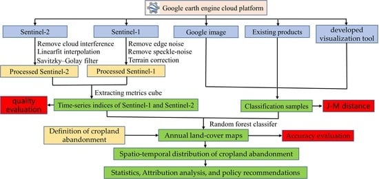
The ground-truth data contained samples of 752 irrigated cropland, 1237 rainfed cropland, 1576 wood vegetation, and 623 herbaceous vegetation from 2019 to 2021. In addition, cloudless GF-2 satellite imagery in July 2020 was obtained in the study area. These data were used to verify the accuracy of the classification and spatial detail.

2.3. Method

The technical flowchart of the study included five steps (Figure 2). The purpose of Step 1 was to extract the metrics of classification after Sentinel-1 and Sentinel-2 processing (Section 2.3.2). Step 2 was to generate pre-classification samples by combining multisource data and timeseries index curves (Section 2.3.3). Step 3 was to produce annual land-cover maps using a random forest classifier (Section 2.3.4). Step 4 was to map cropland abandonment with different types and degrees according to the class definition (Section 2.3.1 and Section 2.3.5). Step 5 was to quantify and evaluate the accuracies and reliability of the method (Section 2.3.6).

2.3.1. Definition of Cropland Abandonment

At present, the definition of abandoned cropland remains controversial around the world. The Food and Agriculture Organization of the United Nations (FAO) defines abandoned cropland as that which has not been cultivated for at least 5 years [45]. In Asia, abandoned cropland has a shorter time boundary due to more frequent land-cover changes. In this study, abandoned cropland referred to areas that were cultivated in the first year but no longer cultivated in the subsequent 2 years [46], which included abandoned irrigated cropland and abandoned rainfed cropland. Correspondingly, active cropland was designated as the areas cultivated for three consecutive years. Intermittent cropland was designated as the areas cultivated for only 2 years among the three consecutive years, which included intermittent irrigated cropland and intermittent rainfed cropland. Herbaceous vegetation was defined as any unplowed area that was not dominated by shrubs or trees. Wood vegetation was defined as areas where shrubs and trees were dominant. The annual land-cover maps enabled the identification of abandoned rainfed cropland and irrigated cropland by assessing land-cover trajectories along with time.

2.3.2. Sentinel-1 and Sentinel-2 Imageries Processing

There is a need for more advanced timeseries analyses on short-term phenological characteristics to extract cropland abandonment in hilly areas. The monthly interval composition method is commonly used in land-cover classification and phenological characteristic analysis. It can effectively utilize the cloudless pixels of the image during the period and reduce interference of clouds and shadows [8,15,24]. Furthermore, we mapped the spatial distribution and calculated the number of available pixels each month in the study area (Figure 3).
Sentinel-1 imagery was preprocessed with thermal noise removal, data calibration, multi-looking, and range-Doppler terrain correction to a resolution of 10 m before being integrated into the GEE data pool. Even with such corrections applied, Sentinel-1 imagery suffered from speckle noise and radiometric distortion. Speckle noise is unique to SAR imagery and is caused by backscatter interferences between adjacent returns. Although images affected by speckle noise show large-scale distinguishable features, they may be seriously compromised at smaller scales. It has been shown that speckle noise may create confusion in machine learning algorithms [47]. Radiometric distortions over rugged terrain within the backscatter products on GEE originate from the side-looking SAR imaging geometry. Such distortions are strong enough to exceed weaker differences of the signal due to variation in land cover [48]. It is, therefore, necessary to account for these effects during the generation of higher-level backscatter products to enable a variety of land applications [49]. In this study, we processed Sentinel-1 on GEE by selecting instrument mode (IW), transmitter–receiver polarization (VV, VH), and ascending orbits. Furthermore, the framework proposed by Adugna Mullissa was used to remove additional border noise, reduce speckle noise, and normalize radiometric terrain (code available at: https://github.com/adugnag/gee_s1_ard, accessed on 22 June 2022).
Level-2A Sentinel-2 surface reflectance (SR) imagery was processed with calibration and atmospheric correction before being integrated into the GEE data pool. In this study, Sentinel-2 imagery was processed by the removal of the interference of cloud and shadow, linear fit interpolation, and Savitzky–Golay filtering. Removing the interference of cloud and shadow is an important step, and a reasonable method can greatly reduce the error in cloudy areas. The bands of SCL, MSK_CLDPRB, and MSK_SNWPRB included in Sentinel-2 were used to remove cloud and shadow. Preliminary experiments informed that when the thresholds of the MSK_CLDPRB band and MSK_SNWPRB band were larger than 20, the removal of some clouds was poor (especially thin clouds). However, when the thresholds of the MSK_CLDPRB band and MSK_SNWPRB band were larger than 10, some urban areas were misidentified as clouds. In addition, the shadow and cirrus values of the SCL band 3 three and 10. By comprehensively using the MSK_CLDPRB band, MSK_SNWPRB band, and SCL band, the thresholds of the MSK_CLDPRB band and MSK_SNWPRB band were set to 15. As a result, the value of the SCL band was no longer equal to 3 and 10, and the optimal cloud removal was achieved. Linear fit interpolation was carried out to fill missing values by properties of “system:time_start”. The code of removing cloud and shadow, and the interpolating value linear fit was akin to the example provided by the SpatialThoughts official website: https://spatialthoughts.com/2021/11/08/temporal-interpolation-gee, accessed on 22 June 2022. The Savitzky–Golay filter is a digital filter that can be applied to a set of images to smooth the image, i.e., to increase the precision of the image without distorting the phenology tendency. This was achieved, in a process known as convolution, by fitting successive subsets of adjacent data points with a low-degree polynomial using the method of linear least squares [50]. Many articles have proven the excellent efficiency of Savitzky–Golay (SG) filtering to reconstruct remote sensing images, especially in areas seriously disturbed by clouds [30,33,51]. The Open Earth Engine Library (OEEL) is an open-source SG filter library which can be easily applied on GEE; an application example is given at https://code.earthengine.google.com/?scriptPath=users/OEEL/examples:MODISFiltering, accessed on 22 June 2022. The moving window of observation was set to three, with a filter order of two, as the growth period of most crops exceeds 3 months [36]. After image processing, a set of commonly used indices were composited by Sentinel-1 and Sentinel-2. A summary of the indices and their expressions is reported in Table 2.

2.3.3. Training and Validation Samples Generation for Classification

The quality of the samples directly determines the reliability of the classification results. On the one hand, the samples must be representative and must be able to represent the characteristics of the features in the study area; on the other hand, the samples must be independent to reduce errors caused by spatial correlation. Google imagery is an important sample source for visual interpretation, where different types of land cover present different shapes, textures, colors, etc. [65]. However, due to the limitation of surface changes and the experience of visual interpreters, the interpretation may be far from accurate. Using existing classification products to select samples has been recognized as a fast and effective method in many articles [52,66,67]. Nevertheless, existing classification products may not perform well in hilly areas, and they can only be used as a preliminary reference. Phenological features are the most common and reliable features of vegetation, and the use of high-temporal spectral changes can adequately characterize vegetation, in order to achieve the goal of identification. However, the phenological feature may be deformed to some extent due to cloud disturbance. In this study, Google imagery was used for visual interpretation, and the GFC, JRC, ESA WorldCover 2020 land cover, global ESRI 2020 land cover, CLCD in 2020, and GLC_FCS30 in 2020 datasets were used to select the same land cover. The study area was divided into 3 km × 3 km grids, and 1–10 samples were obtained in each grid [68,69]. Then, the multiple indices of GCVI, NDVI, EVI, LSWI, BSI, NBR, NDWI, VV, and VH timeseries were used to match the phenological characteristics of the land cover by applying the developed timeseries viewer tool of GEE [1]. With the two steps above, a set of samples for pre-classification was obtained.

2.3.4. Annual Land-Cover Classification

The samples were split randomly in the ratio of 7:3 for training and validation respectively. The random forest (RF) classifier was selected to map both pre-classification and the secondary classification, as it has been successfully used in a variety of satellite-based applications including crop type mapping, with the valuable advantage of being intrinsically not prone to overfitting [70,71,72]. More importantly, the implementation of RF is available in GEE, allowing large-scale predictions at the pixel level. As with many other models, RF is sensitive to the choice of hyperparameters and the training data used [73]. On the basis of several fitting experiments, the number of random forest trees was set to 250 to achieve better accuracy in this study. Following pre-classification for three consecutive years, the spatial distribution of six categories of features was obtained, namely, irrigated cropland, rainfed cropland, woody vegetation, herbaceous vegetation, water bodies, and impervious surfaces. The total area of non-vegetation type cover (i.e., water bodies and impervious surfaces) for three consecutive years was masked so that only vegetation cover types remained. The samples with consistent results from three consecutive years of pre-classification were selected for secondary classification. During pre-classification, the non-vegetated areas of the image were masked, and stable and reliable training samples were obtained. Using the masked image and samples for classification, the spatial distribution of land cover was obtained for each year for irrigated cropland, rainfed cropland, woody vegetation, and herbaceous vegetation. Following pre-classification screening, accurate vegetation regions were identified, while the stable pixels obtained from the results of pre-classification for three consecutive years were expanded using the samples of secondary classification to increase the reliability of the samples. Through the above steps, the spatial distribution of the vegetation region in the study area was generated for three consecutive years.

2.3.5. Mapping Spatial Distribution of Cropland Abandonment

On the basis of the definition of abandoned cropland and annual land-cover classification, the spatial distribution of cropland abandonment with rainfed cropland and irrigated cropland was mapped. Abandoned cropland was considered for areas out of cultivation for 2 years, and strong land policy support is required to improve the situation. Special attention is required for the potential abandonment of intermittent cropland. Active cropland represented areas always under cultivation, which serve as an important safeguard for food production. According to the area and proportion of cropland abandonment, reasonable adjustment and planning of the cropland will be carried out in future work.

2.3.6. Accuracy Assessment

The verification samples were divided into two categories; one was obtained using our method (Section 2.3.3 and Section 2.3.4), and the other constituted field samples (Section 2.2.3). On the basis of the validation samples, confusion matrices were created, and the max, min, and mean of producer accuracy (PA), user accuracy (UA), and overall accuracy (OA), as well as the kappa coefficient, were calculated for the 3 years. The F1 score (F1 = 2 × UA × PA (UA + PA)), a harmonic mean of user and producer accuracy, was calculated. It ranges from 0 to 1 with a higher score indicating better classification performance, and it is advantageous when learning from imbalanced data [74]. The classification results were compared with existing classification products, highlighting the classification accuracy and spatial detail in the study area.

3. Results

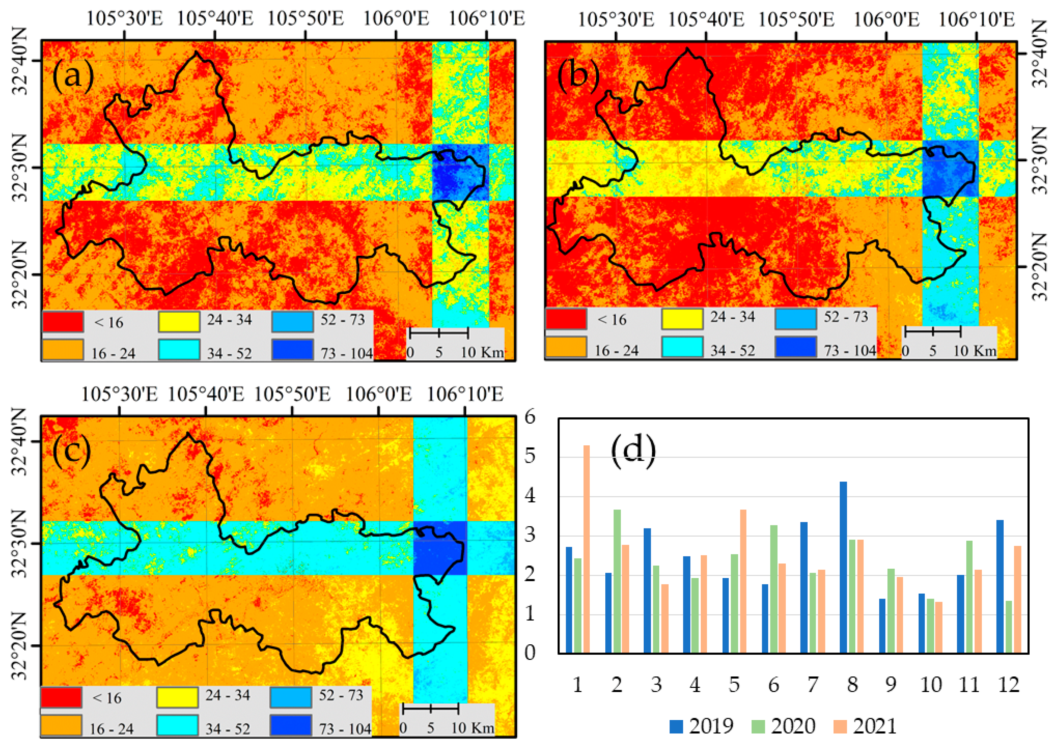
3.1. Usability Assessment of Imagery Processing

To ensure the imagery quality for accurate classification, the median value of NDVI was chosen to assess the accuracy of the processed images. Next, the standard deviation was calculated to assess the effect of cloud interference. It was expected that a larger standard deviation would indicate more severe cloud interference.
The results showed that the median of NDVI showed good variation in phenological characteristics, with no abrupt changes in standard deviation produced, indicating good results from the processed image (Figure 4). These statistical results demonstrated that the image quality was significantly improved after cloud interference removal, linear interpolation, and SG filtering.

3.2. Separability Assessment of Samples

The Jeffries–Matusita (JM) distance between a pair of probability functions is a measure of the average distance between the two class density functions [75]. The JM distance between the two classes was closer to 2, indicating a classification accuracy. All the samples were generated in a grid-by-grid manner, whose spatial autocorrelation was reduced, and whose reliability was improved. After calculation, the JM distances of different samples were greater than 1.85 in this study, indicating that the reliability of sample quality was enhanced.

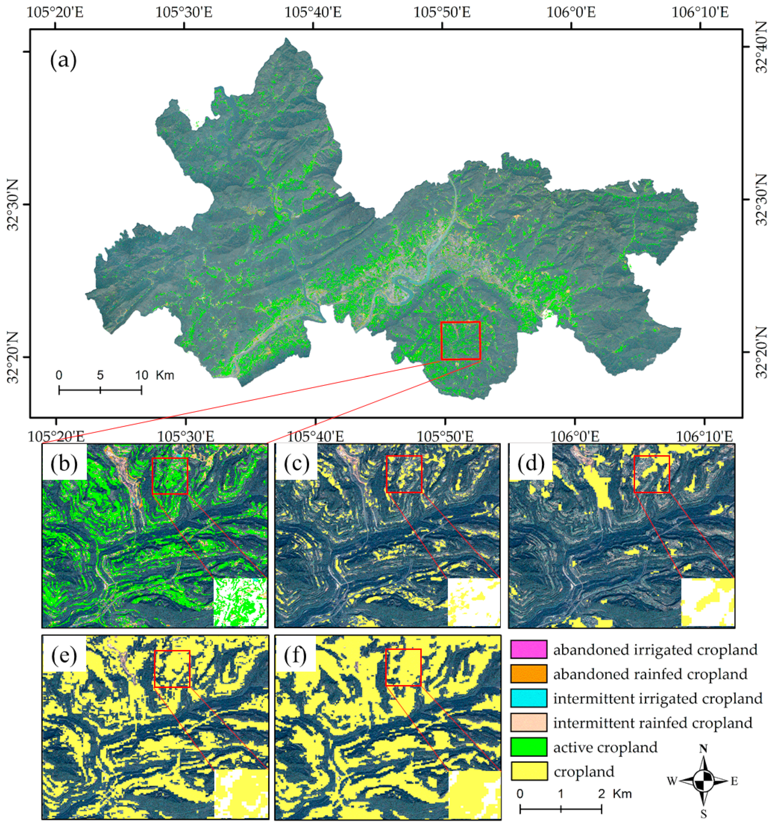
3.3. Spatial Distribution and Statistics of Cropland Abandonment

Visually, the cropland was mainly located near rivers and residential areas, with a greater concentration in urban centers and greater dispersion in remote areas. Small cropland fields (<1 ha) and small-holder agriculture were prevalent in the study area (Figure 5).
The areas and percentages of active cropland, intermittent irrigated cropland, intermittent rainfed cropland, abandoned irrigated cropland, and abandoned rainfed cropland were calculated (Table 3). In general, the area of abandoned cropland had a high proportion, and the abandoned rainfed cropland was the most obvious. In addition, the intermittently abandoned cropland had a high proportion, indicating that the area of cropland abandonment tended to expand in the study area.

3.4. Accuracy Assessment of Annual Land-Cover Maps

The accuracies of annual land-cover maps were quantified from 2019 to 2021. Firstly, the classification result was validated using the samples obtained by our method. The result showed that the overall accuracies ranged from 0.895 to 0.902, with the kappa ranged from 0.851 to 0.862. The F1 scores of irrigated cropland, rainfed cropland, woody vegetation, and herbaceous vegetation ranged from 0.836 to 0.879, 0.759 to 0.8, 0.964 to 0.981, and 0.958 to 0.978, respectively. Then, some field samples were selected to validate the classification results. The results show that the overall accuracy and kappa accuracy ranged from 0.902 to 0.921 and from 0.87 to 0.895, respectively. The F1 score of irrigated cropland, rainfed cropland, woody vegetation, and herbaceous vegetation ranged from 0.863 to 0.902, from 0.781 to 0.813, from 0.971 to 0.990, and from 0.961 to 0.980, respectively (Figure 6). By comparing the classification accuracy of the samples obtained using our method with field samples, the results showed good agreement, thus affirming the reliability of our method in terms of classification accuracy.

4. Discussion

4.1. Comparison of Classification Accuracy with Existing Products

Through field survey collection and statistics, the cropland area of the field data in the study area was determined. The total area of cropland was calculated by merging abandoned, intermittent, and active cropland, which was compared with the area of cropland in the existing classification products. The results of different products were compared with the field data as a reference, as shown in Table 4. The results showed that the cropland areas of our method had the lowest deviation from the field data. The ESA WorldCover 2020 and the ESRI land cover 2020 underestimated the areas of cropland in the study area. By superimposing with the GF-2 imagery, it can be found that many small farmlands were missed, and the ESRI land cover still had obvious misclassification (Figure 5c,d). In contrast, the GLCF_FCS30 and the CLCD in 2020 overestimated the areas of cropland in the study area. The results showed that some of the woodland areas were misclassified as cropland areas (Figure 5e,f). In our method, irrigated cropland F1 scores exceeded 0.836 and rainfed cropland F1 scores exceeded 0.759, which outperformed the existing products.

4.2. The Spatial Distribution, Attribution, and Policy Recommendations for Cropland Abandonment

As shown in Table 3, the rainfed cropland occupied around 94% of the abandoned cropland, while the irrigated cropland accounted for only a small portion. Furthermore, most of the abandoned irrigated cropland fields were small, and there was no large-scale abandonment, whilst the abandoned rainfed cropland exhibited a certain degree of aggregation. The intermittent cropland was often distributed adjacent to abandoned cropland, with the possibility of abandonment. Intermittent cropland and abandoned cropland aggravated the spatial distribution of agglomeration, which posed a hidden danger to food security. Active cropland had the highest concentration, usually located around rivers and near settlements (Figure 5).
Our study found that the causes of cropland abandonment were influenced by both the impact of human activities and the natural environment. Firstly, rural–urban migration led to a shortage of labor for agricultural activities, especially in economically underdeveloped areas, which was the main reason for cropland abandonment. Secondly, the abandonment rate of rainfed cropland was much higher than that of irrigated cropland, which indicated that some arid areas were not suitable for cultivation. Lastly, the fragmentation of arable plots inhibited large-scale cultivation; thus, the agricultural input-output ratio was low.
Given the distribution of abandoned cropland in the study area, the government should take targeted measures to improve the use of cropland. Firstly, the government should further increase the subsidies for rural farming and narrow the income gap between urban migrant workers and agricultural laborers. Secondly, appropriate land-use conversion should be carried out for the rainfed cropland unsuitable for cultivation. Lastly, the government should establish a corresponding system of cropland transfer to reduce the fragmentation of cropland caused by human factors, strengthen the agglomeration of scattered cropland, and improve the farming input–output ratio.

4.3. The Effect of Terrain Correction on Classification Results

For hilly areas, variations in topographic relief can cause differences in backscatter coefficients and affect the accuracy of land-cover classification. Many studies have shown that topographic correction is the key to Sentinel-1 imagery processing [76,77,78]. In this study, we used the Sentinel-1 data processing process developed based on GEE, which included topographic correction [37]. The method depended on the angular relationships between the SAR imagery and the terrain geometry. We selected the NASA SRTM Digital Elevation 30 m as auxiliary data for terrain correction (data available at: https://developers.google.com/earth-engine/datasets/catalog/USGS_SRTMGL1_003?hl=en, accessed on 22 June 2022). The topography-corrected Sentinel-1 imagery improved the classification results by 0.006 to 0.024 in overall accuracy. For the coverage category, the extraction was most pronounced for irrigated cropland, where the Sentinel-1 responding to water bodies was most significant during the irrigation period.

4.4. Method Transferability and Improvement

Our approach provided a large degree of improvement in solving the problem of abandoned cropland in hilly areas. On the one hand, we obtained good available images at a monthly scale through cloudy interference removal, interpolation, and SG filtering. On the other hand, we improved efficiency by obtaining reliable samples through multisource data filtering and developed a visualization tool for GEE. The annual land-cover results were obtained by pre-classification and secondary classification, and then the definition was used to generate the final spatial distribution of cropland abandonment. However, additional adjustment may be needed according to local phenological characteristics, as also applied in other regions. For example, in this study, the abandoned cropland refers to areas not cultivated for two consecutive years, while the FAO defines it as cropland that has not been cultivated for more than 5 years. In addition, the timeseries window of the SG filter can be modified according to the degree of the impact image. There is still some room for improvement in our method. When a single optical remote sensing image is disturbed by clouds for a long period, the fill-and-fit (FF) approach may not be sufficient for surface phenology monitoring. It is necessary to use other images for filling in and to ensure a sufficient number of observations to effectively extract surface coverage changes. With the successful launch of Landsat-9, remote sensing images of each scene for 8 days can be jointly acquired with Landsat-8. Combining the timeseries of Landsat and Sentinel will increase the availability of remote sensing imagery in hilly areas. Furthermore, with the further development of the GEE platform, more reliable algorithms and data with higher precision will be available to improve the accuracy of cropland abandonment. In the future, free and publicly accessible images with a higher spatial resolution can reduce the influence of mixed pixels in hilly areas, as well as ameliorate the reliability of classification results.

5. Conclusions

The monitoring of cropland abandonment in hilly areas is a key but difficult task in the land-cover change field, and there is a lack of reliable and efficient approaches to monitor cropland abandonment in hilly areas on large scale. In this study, we presented an approach combining Sentinel-1 and Sentinel-2 imageries and incorporating them into the GEE platform to determine cropland abandonment on the basis of annual classification. Firstly, cloud interference removal, linear interpolation, and SG filtering were applied to synthesize the eligible indices with monthly intervals. Secondly, high-quality samples were generated using superimposed Google imagery, existing classification products, and developed visualization tools of GEE. Then, the RF classifier was used to perform pre-classification and secondary classification, resulting in annual land-cover distribution maps. Lastly, cropland abandonment of rainfed cropland and irrigated cropland was mapped in the study area as per the designated definition of cropland abandonment. Our work sheds some light on mapping the cropland abandonment in hilly areas on a global scale.

Author Contributions

S.H., conceptualization, data curation, methodology, writing—original draft, and writing—review and editing; H.S., conceptualization, funding acquisition, methodology, writing—review and editing, and project administration; W.X., conceptualization and funding acquisition; Z.Y., writing—review and editing; M.Y., investigation and data curation; J.Z., investigation; J.Q., conceptualization. All authors have read and agreed to the published version of the manuscript.

Funding

This study was supported by the National Natural Science Fund of China (Grant No. 41401659), the Science and Technology Department of Sichuan Province (Grant No. 2015JY0145), and the Natural Resources Department of Sichuan Province (Grant No. kj-2021-5).

Data Availability Statement

Sentinel-1, Sentinel-2, Google image, Global Forest Change (GFC) land cover, the JRC annual water surface data, the ESA WorldCover 2020 land cover, and global ESRI 2020 land cover data are available via the Google Earth Engine platform. The Global land cover product with a fine classification system at 30 m (GLC_FCS30) in 2020 is available via the Earth Science Big Data Science Engineering Data Sharing Service System. The China Land Cover Dataset (CLCD) in 2020 is available via the website https://zenodo.org/record/5210928#.YqB5whpByUl, accessed on 22 June 2022.

Conflicts of Interest

The authors declare no conflict of interest.

References

  1. Yin, H.; Brandão, A.; Buchner, J.; Helmers, D.; Iuliano, B.G.; Kimambo, N.E.; Lewińska, K.E.; Razenkova, E.; Rizayeva, A.; Rogova, N.; et al. Monitoring cropland abandonment with Landsat time series. Remote Sens. Environ. 2020, 246, 111873. [Google Scholar] [CrossRef]
  2. Min, R.; Yang, H.; Mo, X.; Qi, Y.; Xu, D.; Deng, X. Does Institutional Social Insurance Cause the Abandonment of Cultivated Land? Evidence from Rural China. Int. J. Environ. Res. Public Health 2022, 19, 1117. [Google Scholar] [CrossRef] [PubMed]
  3. Romero-Calcerrada, R.; Perry, G.L.W. The role of land abandonment in landscape dynamics in the SPA ‘Encinares del río Alberche y Cofio, Central Spain 1984–1999. Landsc. Urban Plan. 2004, 66, 217–232. [Google Scholar] [CrossRef]
  4. Knoke, T.; Calvas, B.; Moreno, S.O.; Onyekwelu, J.C.; Griess, V.C. Food production and climate protection—What abandoned lands can do to preserve natural forests. Glob. Environ. Change 2013, 23, 1064–1072. [Google Scholar] [CrossRef]
  5. Kurganova, I.; de Gerenyu, V.L.; Kuzyakov, Y. Large-scale carbon sequestration in post-agrogenic ecosystems in Russia and Kazakhstan. Catena 2015, 133, 461–466. [Google Scholar] [CrossRef]
  6. Lesschen, J.P.; Cammeraat, L.H.; Kooijman, A.M.; van Wesemael, B. Development of spatial heterogeneity in vegetation and soil properties after land abandonment in a semi-arid ecosystem. J. Arid Environ. 2008, 72, 2082–2092. [Google Scholar] [CrossRef]
  7. Sieber, A.; Uvarov, N.V.; Baskin, L.M.; Radeloff, V.C.; Bateman, B.L.; Pankov, A.B.; Kuemmerle, T. Post-Soviet land-use change effects on large mammals’ habitat in European Russia. Biol. Conserv. 2015, 191, 567–576. [Google Scholar] [CrossRef]
  8. He, S.; Shao, H.; Xian, W.; Zhang, S.; Zhong, J.; Qi, J. Extraction of Abandoned Land in Hilly Areas Based on the Spatio-Temporal Fusion of Multi-Source Remote Sensing Images. Remote Sens. 2021, 13, 3956. [Google Scholar] [CrossRef]
  9. Alcantara, C.; Kuemmerle, T.; Prishchepov, A.V.; Radeloff, V.C. Mapping abandoned agriculture with multi-temporal MODIS satellite data. Remote Sens. Environ. 2012, 124, 334–347. [Google Scholar] [CrossRef]
  10. Alcantara, C.; Kuemmerle, T.; Baumann, M.; Bragina, E.V.; Griffiths, P.; Hostert, P.; Knorn, J.; Müller, D.; Prishchepov, A.V.; Schierhorn, F.; et al. Mapping the extent of abandoned farmland in Central and Eastern Europe using MODIS time series satellite data. Environ. Res. Lett. 2013, 8, 035035. [Google Scholar] [CrossRef]
  11. Zhu, X.; Xiao, G.; Zhang, D.; Guo, L. Mapping abandoned farmland in China using time series MODIS NDVI. Sci. Total Environ. 2020, 755, 142651. [Google Scholar] [CrossRef]
  12. Prishchepov, A.V.; Radeloff, V.C.; Baumann, M.; Kuemmerle, T.; Müller, D. Effects of institutional changes on land use: Agricultural land abandonment during the transition from state-command to market-driven economies in post-Soviet Eastern Europe. Environ. Res. Lett. 2012, 7, 024021. [Google Scholar] [CrossRef]
  13. Yin, H.; Prishchepov, A.V.; Kuemmerle, T.; Bleyhl, B.; Buchner, J.; Radeloff, V.C. Mapping agricultural land abandonment from spatial and temporal segmentation of Landsat time series. Remote Sens. Environ. 2018, 210, 12–24. [Google Scholar] [CrossRef]
  14. Levers, C.; Schneider, M.; Prishchepov, A.V.; Estel, S.; Kuemmerle, T. Spatial variation in determinants of agricultural land abandonment in Europe. Sci. Total Environ. 2018, 644, 95–111. [Google Scholar] [CrossRef]
  15. Yoon, H.; Kim, S. Detecting abandoned farmland using harmonic analysis and machine learning. ISPRS J. Photogramm. Remote Sens. 2020, 166, 201–212. [Google Scholar] [CrossRef]
  16. Veloso, A.; Mermoz, S.; Bouvet, A.; Le Toan, T.; Planells, M.; Dejoux, J.-F.; Ceschia, E. Understanding the temporal behavior of crops using Sentinel-1 and Sentinel-2-like data for agricultural applications. Remote Sens. Environ. 2017, 199, 415–426. [Google Scholar] [CrossRef]
  17. Gorelick, N.; Hancher, M.; Dixon, M.; Ilyushchenko, S.; Thau, D.; Moore, R. Google Earth Engine: Planetary-scale geospatial analysis for everyone. Remote Sens. Environ. 2017, 202, 18–27. [Google Scholar] [CrossRef]
  18. Hansen, M.C.; Potapov, P.V.; Moore, R.; Hancher, M.; Turubanova, S.A.; Tyukavina, A.; Thau, D.; Stehman, S.V.; Goetz, S.J.; Loveland, T.R.; et al. High-Resolution Global Maps of 21st-Century Forest Cover Change. Science 2013, 342, 850–853. [Google Scholar] [CrossRef] [Green Version]
  19. Pekel, J.F.; Cottam, A.; Gorelick, N.; Belward, A.S. High-resolution mapping of global surface water and its long-term changes. Nature 2016, 540, 418–422. [Google Scholar] [CrossRef]
  20. Zanaga, D.; Van De Kerchove, R.; De Keersmaecker, W.; Souverijns, N.; Brockmann, C.; Quast, R.; Wevers, J.; Grosu, A.; Paccini, A.; Vergnaud, S.; et al. ESA WorldCover 10 m 2020 v100. Zenodo 2021. [Google Scholar] [CrossRef]
  21. Karra, K.; Kontgis, C.; Statman-Weil, Z.; Mazzariello, J.C.; Mathis, M.; Brumby, S.P. Global land use/land cover with Sentinel 2 and deep learning. In Proceedings of the 2021 IEEE International Geoscience and Remote Sensing Symposium IGARSS, Brussels, Belgium, 11–16 July 2021; pp. 4704–4707. [Google Scholar]
  22. Kruitwagen, L.; Story, K.T.; Friedrich, J.; Byers, L.; Skillman, S.; Hepburn, C. A global inventory of photovoltaic solar energy generating units. Nature 2021, 598, 604–610. [Google Scholar] [CrossRef]
  23. Liu, X.; Hu, G.; Chen, Y.; Li, X.; Xu, X.; Li, S.; Pei, F.; Wang, S. High-resolution multi-temporal mapping of global urban land using Landsat images based on the Google Earth Engine Platform. Remote Sens. Environ. 2018, 209, 227–239. [Google Scholar] [CrossRef]
  24. Wuyun, D.; Sun, L.; Sun, Z.; Chen, Z.; Hou, A.; Teixeira Crusiol, L.G.; Reymondin, L.; Chen, R.; Zhao, H. Mapping fallow fields using Sentinel-1 and Sentinel-2 archives over farming-pastoral ecotone of Northern China with Google Earth Engine. GIScience Remote Sens. 2022, 59, 333–353. [Google Scholar] [CrossRef]
  25. Zurita-Milla, R.; Clevers, J.; Schaepman, M.E. Unmixing-Based Landsat TM and MERIS FR Data Fusion. IEEE Geosci. Remote Sens. Lett. 2008, 5, 453–457. [Google Scholar] [CrossRef] [Green Version]
  26. Zhu, X.; Chen, J.; Gao, F.; Chen, X.; Masek, J.G. An enhanced spatial and temporal adaptive reflectance fusion model for complex heterogeneous regions. Remote Sens. Environ. 2010, 114, 2610–2623. [Google Scholar] [CrossRef]
  27. Li, A.; Bo, Y.; Zhu, Y.; Guo, P.; Bi, J.; He, Y. Blending multi-resolution satellite sea surface temperature (SST) products using Bayesian maximum entropy method. Remote Sens. Environ. 2013, 135, 52–63. [Google Scholar] [CrossRef]
  28. Song, H.; Liu, Q.; Wang, G.; Hang, R.; Huang, B. Spatiotemporal Satellite Image Fusion Using Deep Convolutional Neural Networks. IEEE J. Sel. Top. Appl. Earth Obs. Remote Sens. 2018, 11, 821–829. [Google Scholar] [CrossRef]
  29. Zhu, X.; Helmer, E.H.; Gao, F.; Liu, D.; Chen, J.; Lefsky, M.A. A flexible spatiotemporal method for fusing satellite images with different resolutions. Remote Sens. Environ. 2016, 172, 165–177. [Google Scholar] [CrossRef]
  30. Chen, J. A simple method for reconstructing a high-quality NDVI time-series data set based on the Savitzky–Golay filter. Remote Sens. Environ. 2004, 91, 332–344. [Google Scholar] [CrossRef]
  31. Yan, L.; Roy, D. Spatially and temporally complete Landsat reflectance time series modelling: The fill-and-fit approach. Remote Sens. Environ. 2020, 241, 111718. [Google Scholar] [CrossRef]
  32. Zhu, X.; Liu, D.; Chen, J. A new geostatistical approach for filling gaps in Landsat ETM+ SLC-off images. Remote Sens. Environ. 2012, 124, 49–60. [Google Scholar] [CrossRef]
  33. Chen, Y.; Cao, R.; Chen, J.; Liu, L.; Matsushita, B. A practical approach to reconstruct high-quality Landsat NDVI time-series data by gap filling and the Savitzky–Golay filter. ISPRS J. Photogramm. Remote Sens. 2021, 180, 174–190. [Google Scholar] [CrossRef]
  34. Zhou, J.; Chen, J.; Chen, X.; Zhu, X.; Qiu, Y.; Song, H.; Rao, Y.; Zhang, C.; Cao, X.; Cui, X. Sensitivity of six typical spatiotemporal fusion methods to different influential factors: A comparative study for a normalized difference vegetation index time series reconstruction. Remote Sens. Environ. 2021, 252, 112130. [Google Scholar] [CrossRef]
  35. Kong, D.; Zhang, Y.; Gu, X.; Wang, D. A robust method for reconstructing global MODIS EVI time series on the Google Earth Engine. ISPRS J. Photogramm. Remote Sens. 2019, 155, 13–24. [Google Scholar] [CrossRef]
  36. Liu, L.; Xiao, X.; Qin, Y.; Wang, J.; Xu, X.; Hu, Y.; Qiao, Z. Mapping cropping intensity in China using time series Landsat and Sentinel-2 images and Google Earth Engine. Remote Sens. Environ. 2020, 239, 111624. [Google Scholar] [CrossRef]
  37. Mullissa, A.; Vollrath, A.; Odongo-Braun, C.; Slagter, B.; Balling, J.; Gou, Y.; Gorelick, N.; Reiche, J. Sentinel-1 SAR Backscatter Analysis Ready Data Preparation in Google Earth Engine. Remote Sens. 2021, 13, 1954. [Google Scholar] [CrossRef]
  38. Vollrath, A.; Mullissa, A.; Reiche, J. Angular-Based Radiometric Slope Correction for Sentinel-1 on Google Earth Engine. Remote Sensing 2020, 12, 1867. [Google Scholar] [CrossRef]
  39. Han, J.; Zhang, Z.; Luo, Y.; Cao, J.; Zhang, L.; Cheng, F.; Zhuang, H.; Zhang, J.; Tao, F. NESEA-Rice10: High-resolution annual paddy rice maps for Northeast and Southeast Asia from 2017 to 2019. Earth Syst. Sci. Data 2021, 21, 5969–5986. [Google Scholar] [CrossRef]
  40. Verhelst, K.; Gou, Y.; Herold, M.; Reiche, J. Improving Forest Baseline Maps in Tropical Wetlands Using GEDI-Based Forest Height Information and Sentinel-1. Forests 2021, 12, 1374. [Google Scholar] [CrossRef]
  41. Dong, D.; Wang, C.; Yan, J.; He, Q.; Wei, Z. Combing Sentinel-1 and Sentinel-2 image time series for invasive Spartina alterniflora mapping on Google Earth Engine: A case study in Zhangjiang Estuary. J. Appl. Remote Sens. 2020, 14, 044504. [Google Scholar]
  42. You, N.; Dong, J. Examining earliest identifiable timing of crops using all available Sentinel 1/2 imagery and Google Earth Engine. ISPRS J. Photogramm. Remote Sens. 2020, 161, 109–123. [Google Scholar] [CrossRef]
  43. Zhang, X.; Liu, L.; Chen, X.; Gao, Y.; Xie, S.; Mi, J. GLC_FCS30: Global land-cover product with fine classification system at 30 m using time-series Landsat imagery. Earth Syst. Sci. Data Discuss. 2020, 13, 2753–2776. [Google Scholar] [CrossRef]
  44. Yang, J.; Huang, X. 30 m annual land cover and its dynamics in China from 1990 to 2019. Earth Syst. Sci. Data 2021, 13, 3907–3925. [Google Scholar] [CrossRef]
  45. Pointereau, P. Analysis of Farmland Abandonment and the Extent and Location of Agricultural Areas That Are Actually Abandoned or Are in Risk to be Abandoned; EUR-OP: Luxembourg, 2008. [Google Scholar]
  46. Navarro, L.M.; Pereira, H.M. Rewilding Abandoned Landscapes in Europe. Ecosystems 2012, 15, 900–912. [Google Scholar] [CrossRef] [Green Version]
  47. Dasari, K.; Anjaneyulu, L.; Jayasri, P.; Prasad, A. Importance of Speckle Filtering in Image Classification of SAR Data. In Proceedings of the 2015 International Conference on Microwave, Optical and Communication Engineering (ICMOCE), Bhubaneswar, India, 18–20 December 2015; IEEE: Piscataway, NJ, USA. [Google Scholar]
  48. Small, D. Flattening Gamma: Radiometric Terrain Correction for SAR Imagery. IEEE Trans. Geosci. Remote Sens. 2011, 49, 3081–3093. [Google Scholar] [CrossRef]
  49. Hoekman, D.H.; Reiche, J. Multi-model radiometric slope correction of SAR images of complex terrain using a two-stage semi-empirical approach. Remote Sens. Environ. 2015, 156, 1–10. [Google Scholar] [CrossRef]
  50. Savitzky, A.; Golay, M.J. Smoothing and differentiation of data by simplified least squares procedures. Anal. Chem. 1964, 36, 1627–1639. [Google Scholar] [CrossRef]
  51. Cao, R.; Chen, Y.; Shen, M.; Chen, J.; Zhou, J.; Wang, C.; Yang, W. A simple method to improve the quality of NDVI time-series data by integrating spatiotemporal information with the Savitzky-Golay filter. Remote Sens. Environ. 2018, 217, 244–257. [Google Scholar] [CrossRef]
  52. Ni, R.; Tian, J.; Li, X.; Yin, D.; Li, J.; Gong, H.; Zhang, J.; Zhu, L.; Wu, D. An enhanced pixel-based phenological feature for accurate paddy rice mapping with Sentinel-2 imagery in Google Earth Engine. ISPRS J. Photogramm. Remote Sens. 2021, 178, 282–296. [Google Scholar] [CrossRef]
  53. He, Y.; Dong, J.; Liao, X.; Sun, L.; Wang, Z.; You, N.; Li, Z.; Fu, P. Examining rice distribution and cropping intensity in a mixed single- and double-cropping region in South China using all available Sentinel 1/2 images. Int. J. Appl. Earth Obs. Geoinf. 2021, 101, 102351. [Google Scholar] [CrossRef]
  54. Gitelson, A.A.; Gritz, Y.; Merzlyak, M.N. Relationships between leaf chlorophyll content and spectral reflectance and algorithms for non-destructive chlorophyll assessment in higher plant leaves. J. Plant Physiol. 2003, 160, 271–282. [Google Scholar] [CrossRef]
  55. Pan, L.; Xia, H.; Yang, J.; Niu, W.; Wang, R.; Song, H.; Guo, Y.; Qin, Y. Mapping cropping intensity in Huaihe basin using phenology algorithm, all Sentinel-2 and Landsat images in Google Earth Engine. Int. J. Appl. Earth Obs. Geoinf. 2021, 102, 102376. [Google Scholar] [CrossRef]
  56. Liu, H.; Gong, P.; Wang, J.; Wang, X.; Ning, G.; Xu, B. Production of global daily seamless data cubes and quantification of global land cover change from 1985 to 2020-iMap World 1.0. Remote Sens. Environ. 2021, 258, 112364. [Google Scholar] [CrossRef]
  57. You, N.; Dong, J.; Huang, J.; Du, G.; Zhang, G.; He, Y.; Yang, T.; Di, Y.; Xiao, X. The 10-m crop type maps in Northeast China during 2017–2019. Sci. Data 2021, 8, 41. [Google Scholar] [CrossRef]
  58. Poortinga, A.; Tenneson, K.; Shapiro, A.; Nquyen, Q.; San Aung, K.; Chishtie, F.; Saah, D. Mapping Plantations in Myanmar by Fusing Landsat-8, Sentinel-2 and Sentinel-1 Data along with Systematic Error Quantification. Remote Sens. 2019, 11, 831. [Google Scholar] [CrossRef] [Green Version]
  59. Huete, A.R.; Liu, H.Q.; Batchily, K.; van Leeuwen, W. A Comparison of Vegetation Indices over a Global Set of TM Images for EOS-MODIS. Remote Sens. Environ. 1997, 59, 440–451. [Google Scholar] [CrossRef]
  60. Diek, S.; Fornallaz, F.; Schaepman, M.E. Barest Pixel Composite for Agricultural Areas Using Landsat Time Series. Remote Sens. 2017, 9, 1245. [Google Scholar] [CrossRef] [Green Version]
  61. McFeeters, S.K. The use of the Normalized Difference Water Index (NDWI) in the delineation of open water features. Int. J. Remote Sens. 2007, 17, 1425–1432. [Google Scholar] [CrossRef]
  62. Steinhausen, M.J.; Wagner, P.D.; Narasimhan, B.; Waske, B. Combining Sentinel-1 and Sentinel-2 data for improved land use and land cover mapping of monsoon regions. Int. J. Appl. Earth Obs. Geoinf. 2018, 73, 595–604. [Google Scholar] [CrossRef]
  63. Moola, W.S.; Bijker, W.; Belgiu, M.; Li, M. Vegetable mapping using fuzzy classification of Dynamic Time Warping distances from time series of Sentinel-1A images. Int. J. Appl. Earth Obs. Geoinf. 2021, 102, 102405. [Google Scholar] [CrossRef]
  64. Wang, Y.; Fang, S.; Zhao, L.; Huang, X.; Jiang, X. Parcel-based summer maize mapping and phenology estimation combined using Sentinel-2 and time series Sentinel-1 data. Int. J. Appl. Earth Obs. Geoinf. 2022, 108, 102720. [Google Scholar] [CrossRef]
  65. Zhao, Q.; Yu, L.; Li, X.; Peng, D.; Zhang, Y.; Gong, P. Progress and Trends in the Application of Google Earth and Google Earth Engine. Remote Sens. 2021, 13, 3778. [Google Scholar] [CrossRef]
  66. Wang, S.; Di Tommaso, S.; Deines, J.M.; Lobell, D.B. Mapping twenty years of corn and soybean across the US Midwest using the Landsat archive. Sci. Data 2020, 7, 307. [Google Scholar] [CrossRef] [PubMed]
  67. Pan, L.; Xia, H.; Zhao, X.; Guo, Y.; Qin, Y. Mapping Winter Crops Using a Phenology Algorithm, Time-Series Sentinel-2 and Landsat-7/8 Images, and Google Earth Engine. Remote Sens. 2021, 13, 2510. [Google Scholar] [CrossRef]
  68. Sazib, N.; Mladenova, I.; Bolten, J. Leveraging the google earth engine for drought assessment using global soil moisture data. Remote Sens. 2018, 10, 1265. [Google Scholar] [CrossRef] [Green Version]
  69. Zhang, M.; Huang, H.; Li, Z.; Hackman, K.O.; Liu, C.; Andriamiarisoa, R.L.; Ny Aina Nomenjanahary Raherivelo, T.; Li, Y.; Gong, P. Automatic high-resolution land cover production in Madagascar using sentinel-2 time series, tile-based image classification and google earth engine. Remote Sens. 2020, 12, 3663. [Google Scholar] [CrossRef]
  70. Breiman, L. Random Forests. Mach. Learn. 2001, 45, 5–32. [Google Scholar] [CrossRef] [Green Version]
  71. Inglada, J.; Arias, M.; Tardy, B.; Hagolle, O.; Valero, S.; Morin, D.; Dedieu, G.; Sepulcre, G.; Bontemps, S.; Defourny, P. Assessment of an Operational System for Crop Type Map Production Using High Temporal and Spatial Resolution Satellite Optical Imagery. Remote Sens. 2015, 7, 12356–12379. [Google Scholar] [CrossRef] [Green Version]
  72. Belgiu, M.; Drăguţ, L. Random forest in remote sensing: A review of applications and future directions. ISPRS J. Photogramm. Remote Sens. 2016, 114, 24–31. [Google Scholar] [CrossRef]
  73. Jin, Z.; Azzari, G.; You, C.; Di Tommaso, S.; Aston, S.; Burke, M.; Lobell, D.B. Smallholder maize area and yield mapping at national scales with Google Earth Engine. Remote Sens. Environ. 2019, 228, 115–128. [Google Scholar] [CrossRef]
  74. Powers, D.M. Evaluation: From precision, recall and F-measure to ROC, informedness, markedness and correlation. arXiv, 2020; arXiv:2010.16061. [Google Scholar]
  75. Schmidt, K.; Skidmore, A. Spectral discrimination of vegetation types in a coastal wetland. Remote Sens. Environ. 2003, 85, 92–108. [Google Scholar] [CrossRef]
  76. Shelestov, A.; Lavreniuk, M.; Vasiliev, V.; Shumilo, L.; Kolotii, A.; Yailymov, B.; Kussul, N.; Yailymova, H. Cloud Approach to Automated Crop Classification Using Sentinel-1 Imagery. IEEE Trans. Big Data 2020, 6, 572–582. [Google Scholar] [CrossRef]
  77. Xu, L.; Zhang, H.; Wang, C.; Zhang, B.; Liu, M. Crop Classification Based on Temporal Information Using Sentinel-1 SAR Time-Series Data. Remote Sens. 2018, 11, 53. [Google Scholar] [CrossRef] [Green Version]
  78. Markert, K.N.; Markert, A.M.; Mayer, T.; Nauman, C.; Haag, A.; Poortinga, A.; Bhandari, B.; Thwal, N.S.; Kunlamai, T.; Chishtie, F.; et al. Comparing Sentinel-1 Surface Water Mapping Algorithms and Radiometric Terrain Correction Processing in Southeast Asia Utilizing Google Earth Engine. Remote Sens. 2020, 12, 2469. [Google Scholar] [CrossRef]
Figure 1. (a) The location of the study areas in China; (b) the location of the study areas in Sichuan provinces; (c) the location of the study areas in Guangyuan city; (d) NASA SRTM digital elevation 30 m; (e) reclass map of GLC_FCS30 in 2020.
Remotesensing 14 03806 g001
Figure 2. Flowchart of extracting abandoned cropland in hilly areas.
Remotesensing 14 03806 g002
Figure 3. The numbers of cloudless pixels of Sentinel-2 image in the study area from 2019 to 2021. (ac) The numbers of cloudless pixels in 2019 to 2021, respectively. (d) The monthly numbers of cloudless pixels from 2019 to 2021.
Remotesensing 14 03806 g003
Figure 4. Monthly median and standard deviation of NDVI from 2019 to 2021.
Remotesensing 14 03806 g004
Figure 5. Spatial distribution map of cropland abandonment, using GF-2 imagery as the background. Abandoned irrigated cropland/abandoned rainfed cropland, intermittent irrigated cropland, intermittent rainfed cropland, and active cropland were the classes considered. (a) Spatial distribution map of rules including active cropland, intermittent irrigated cropland, intermittent rainfed cropland, abandoned irrigated cropland, and abandoned rainfed cropland in the study area. (b) Partial enlargement of (a). (cf) Corresponding partial enlargements of the ESA WorldCover 2020 land cover product, the global ESRI 2020 land cover product, the GLC_FCS30 in 2020, and the CLCD in 2020; yellow represents the spatial distribution of cropland.
Remotesensing 14 03806 g005
Figure 6. The mean of F1 score, overall accuracy, and kappa from 2019 to 2021. Error bars indicate the min and max intervals.
Remotesensing 14 03806 g006
Table 1. Band information of Sentinel-1 and Sentinel-2.
SatelliteBandsDescriptionsResolution (d/m)
Sentinel-1IW-VV5.405 GHz6/10
IW-VH5.405 GHz
Sentinel-2Band 2—Blue496.6 (A)/492.1 (B)5/10
Band 3—Green560 (A)/559 (B)
Band 4—Red664.5 (A)/665 (B)
Band 8—NIR835.1 (A)/833 (B)
Band 12—SWIR22202.4 (A)/2185.7 (B)5/20
SLCScene classification map
MSK_CLDPRBCloud probability map
MSK_SNWPRBSnow probability map5/10
Table 2. Spectral indices and their expressions from Sentinel-1 and Sentinel-2.
IndicatorsExpressionsReferences
GCVI ρ NIR ρ Green 1 [52,53,54]
NDVI ρ NIR ρ Red ρ NIR + ρ Red [1,36,52,53,55,56,57,58]
EVI 2.5 × ρ NIR ρ Red   ρ NIR + 6.0 ρ Red 7.5 ρ Blue + 1 [52,53,57,59]
LSWI ρ NIR ρ SWIR 2 ρ NIR + ρ SWIR 2 [36,52,53,55,57]
BSI ρ SWIR 2 + ρ Red ρ NIR   ρ Blue ρ SWIR 2 + ρ Red + ρ NIR ρ Blue [1,52,60]
NBR ρ NIR ρ SWIR 2 ρ NIR + ρ SWIR 2   [1,56,58]
NDWI ρ Green ρ NIR ρ Green + ρ NIR [15,53,58,61]
VVSingle co-polarization, vertical transmit/vertical receive[53,62,63,64]
VHDual-band cross-polarization, vertical transmit/horizontal receive[53,62,63,64]
Table 3. The area and percentage of active cropland, intermittent cropland, and abandoned cropland.
Area (km2)Percentage (%)
Active cropland137.477.8
Intermittent irrigated cropland3.01.7
Intermittent rainfed cropland19.811.2
Abandoned irrigated cropland0.90.5
Abandoned rainfed cropland15.58.8
Total176.6100
Table 4. Cropland area statistics of different products.
Area (km2)Field DataOur MethodESAESRIGLC_FCS30CLCD
Cropland180.2176.680.846.3337.2377.5
Publisher’s Note: MDPI stays neutral with regard to jurisdictional claims in published maps and institutional affiliations.

