UAV-Based Hyperspectral Imagery for Detection of Root, Butt, and Stem Rot in Norway Spruce

Abstract

Numerous species of pathogenic wood decay fungi, including members of the genera Heterobasidion and Armillaria, exist in forests in the northern hemisphere. Detection of these fungi through field surveys is often difficult due to a lack of visual symptoms and is cost-prohibitive for most applications. Remotely sensed data can offer a lower-cost alternative for collecting information about vegetation health. This study used hyperspectral imagery collected from unmanned aerial vehicles (UAVs) to detect the presence of wood decay in Norway spruce (Picea abies L. Karst) at two sites in Norway. UAV-based sensors were tested as they offer flexibility and potential cost advantages for small landowners. Ground reference data regarding pathogenic wood decay were collected by harvest machine operators and field crews after harvest. Support vector machines were used to classify the presence of root, butt, and stem rot infection. Classification accuracies as high as 76% with a kappa value of 0.24 were obtained with 490-band hyperspectral imagery, while 29-band imagery provided a lower classification accuracy (~60%, kappa = 0.13).

1. Introduction

Root, butt, and stem rot (RBSR) is a group of fungal diseases that is one of the most significant forest health issues in Europe and throughout the northern hemisphere. RBSR is primarily characterized by the decay of tree roots and the lower tree bole, which can result in reduced tree growth and ultimately lead to tree mortality. In Norway, over 80% of RBSR is caused by fungi from the genera Heterobasidion and Armillaria [1]. Most of the losses occur in forests of Norway spruce (Picea abies L. Karst). Two species in the Heterobasidion genus exist in Norway: Heterobasidion parviporum (Niemelä & Korhonen 1998) and H. annosum s.s. H. parviporum is more common in Norway and primarily infects spruce trees, although pines are also somewhat susceptible, while H. annosum s.s. occurs more often in pine than in spruce. Both species spread via spores and mycelia. Spores can land on tree wounds caused by logging or storm damage, which allows the fungus to spread to healthy stands of trees. Once a tree is infected, the fungus can spread through the root network to adjacent trees (although not directly through the soil) [2].

Armillaria species account for a smaller but significant portion of RBSR infection in Norway. Compared to Heterobasidion, Armillaria tend to cause more significant hollowing of the tree bole but are generally limited to a maximum height of 2 m. In comparison, Heterobasidion may extend as high as 7 m within the stem. Other fungal species which may cause RBSR in Norway include Stereum sanguinolentum (Alb. & Schwein.) Fr., Phellinus chrysoloma (Fr.) Donk, and Climacocystis borealis (Fr.) Kotl. & Pouzar [3]. These species are generally believed to account for a small proportion of RBSR cases in Norway. However, Phellinus chrysoloma can account for a large proportion of infection in high-elevation spruce forests.

In Norway, RBSR is responsible for an estimated 10 million euros in losses for the forest products industry every year, while Europe-wide losses have been estimated at over 800 million euros annually [1,2]. Some losses occur due to the reduction in wood quality in infected trees: logs that could otherwise be used as sawtimber may become pulpwood or biomass feedstock instead, reducing the price forest owners receive for the wood. In contrast, other losses occur due to reduced volume growth and tree death. While H. parviporum, the most common RBSR pathogen in Norway, is rarely fatal (and only after several decades of infection), H. annosum s.s. and H. irregulare both cause tree mortality. The latter is also an invasive pathogen in Europe and other places around the world, with the potential to cause severe ecological damage. There is significant interest in monitoring the presence of these fungi to facilitate control methods, both for ecological and financial reasons. Unfortunately, detecting RBSR infection in the field can be difficult or impossible until the very late stages of infection, and the cost of fieldwork can make effective monitoring programs cost-prohibitive for large areas [4].

One approach for reducing the cost of monitoring programs is the use of remotely sensed data. Remote sensing platforms such as satellites, fixed-wing aircraft, and UAVs facilitate the collection of wall-to-wall data throughout an area of interest, something which is either impractical or impossible with field surveys. These platforms allow for the use of cameras that detect infrared light, making possible the detection of changes in vegetation properties that are invisible to the naked eye. Changes in cellular structure due to stress are usually apparent in the near-infrared (NIR) portion of the spectrum [5], while changes in foliar water content are shown in the shortwave infrared (SWIR) [6]. Consequently, remote sensing can replace expensive sampling methods such as tree coring or felling, which may be necessary to detect pathogens in the field.

Previous research has examined the use of remotely sensed data for more broadly studying a variety of plant pathogens and health issues. Much of the work has focused on the use of passive spectral cameras, both multi-spectral and hyperspectral. Multi-spectral sensors have been more widely utilized due to their lower cost, while hyperspectral sensors offer the advantages of collecting information across a wider portion of the electromagnetic spectrum and of providing finer spectral resolution. Some studies have also incorporated airborne laser scanning (ALS) data to provide information about changes to crown density and other structural properties of trees. Leckie et al. used a multi-spectral sensor with 2.5 m resolution to detect jack pine budworm in Ontario, Canada [7]. They found that classification models using just three bands (red, NIR, and SWIR bands) could provide classification accuracies greater than 80%. Meng et al., used hyperspectral imagery and ALS data to detect defoliation in a mixed-pine oak forest due to gypsy moth infestation [8]. Their analysis used regression models to predict the amount of defoliation, with the best models delivering R² values of 0.81. From the hyperspectral imagery, red-edge and near-infrared bands proved to be the most useful for detecting defoliation.

A few studies have specifically examined spectral information’s use for detecting root and stem rot fungi in woody plants. Examples include Leckie et al., who classified the severity of Phellinus weirii infection in Douglas fir with accuracies as high as 80%, and LeLong et al., who detected the presence of Ganoderma in oil palm [7,9]. This work shows that detecting root rot diseases with remote sensing is possible. An important caveat is that both of these diseases cause significant changes in tree foliage, which are visible to the naked eye, which is not generally true of RBSR in Norway spruce. Kankaanhuhta et al. attempted to detect the presence of RBSR in forests in Finland [10]. They had some success with detecting Heterobasidion in pine forests, but not in spruce, a disparity which is likely due to the greater effect on foliage color in pine trees. Thus, current field-based studies of RBSR detection cannot settle the question of whether pre-visual detection is possible.

Calamita et al. used a laboratory-based hyperspectral camera to classify grape leaves based on the presence of Armillaria in the grapevine of origin [11]. They found significant differences around 705 nm (the red edge) and 550 nm. They were able to identify both visibly diseased and infected but visually asymptomatic plants with an accuracy of 90% and 75%, respectively. This indicates that Armillaria does affect the spectral properties of at least some woody plants. However, it leaves open the question of whether such differences will be noticeable in a field setting. Allen et al. classified the presence of RBSR in spruce trees at a site in Norway using hyperspectral imagery with two different classifiers [12]. Results from this study indicated that detection of RBSR in spruce trees is possible, although classification accuracies were modest (64%).

UAV-based sensors offer several advantages over sensors mounted on conventional fixed-wing aircraft. UAVs can be deployed more rapidly and at a lower cost for very small areas (although costs are higher for large areas). UAVs also allow for more rapid deployment in response to favorable weather conditions. The low flying height of UAVs allows for higher spatial resolution than airborne systems. High spatial resolution UAV imagery has been found to allow for the detection of finer scale variation in plant health than is possible with satellite-based or airborne sensors [13]. Overall, UAVs are highly suitable for gathering remotely sensed data on small tracts of land and provide valuable information for forest owners to aid in management decisions.

Numerous studies have examined using UAV-based sensors to monitor forest pathogens and other health issues. Otsu et al. detected pine processionary moth defoliation in Spain using a combination of Landsat 8 and multi-spectral UAV imagery [14]. Zhang et al. predicted the extent of defoliation on Pinus tabulaeformis Carrière due to the Chinese pine caterpillar using data from a UAV-based hyperspectral camera [15]. Lin et al. used hyperspectral imagery and ALS data to predict damage from pine shoot beetle in Yunnan pine [16]. Their study found that hyperspectral imagery-based estimates of chlorophyll levels and ALS intensity metrics were the most significant predictors of pine shoot beetle infestation. Näsi et al. used a hyperspectral camera with a spectral range of 500–900 nm to classify Norway spruce trees based on bark beetle infection status (healthy, infested, dead) with an overall accuracy of 76% [17]. Subsequent work showed that UAV imagery delivered greater classification accuracies than satellite imagery, likely due to the finer spatial resolution of the UAV imagery [18]. Honkavaara et al. used multitemporal hyperspectral and multi-spectral imagery to attempt to detect RBSR and European spruce beetle attacks at a site in Finland. Their work focused specifically on detecting beetle infestation before any visible changes in foliage color had occurred, rather than beetle infestation with visible foliar symptoms. The overall accuracy obtained in their study was around 45%, although their study used a relatively small sample size, which could have limited the accuracy of their models. While RBSR-infected trees were included in their classification, detecting RBSR was not their study’s primary goal [19].

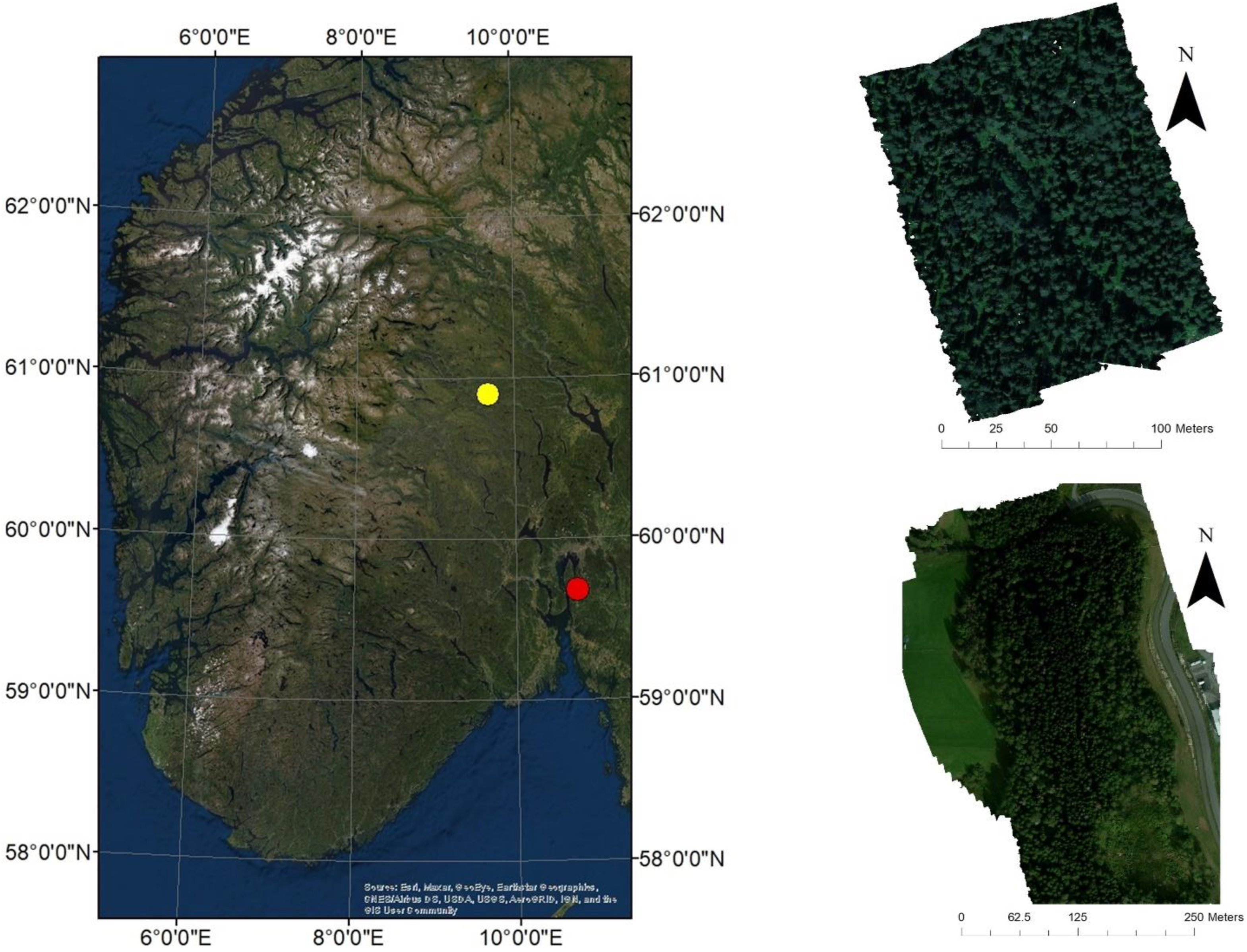
The primary objective of this study was to assess the potential of remotely sensed data from UAV-based cameras to facilitate the detection of RBSR in Norway Spruce by producing classification models. Unlike most previous studies of UAV applications in forest pathology, this study focused solely on pre-visual detection of infection since RBSR rarely produces visible changes to foliage in Norwegian conditions. Two cameras were used, allowing for a comparison between two sensor types. With the use of two sensors, it was hoped that the effect of different spectral regions or numbers of spectral bands on the accuracy of classification could be assessed. Since the cameras used in this study covered different wavelength regions, resampling was also performed on one of the images to enable such comparisons. Based on the spectral data collected from the imagery, trees were classified according to rot infection status. The second major objective of the study was to determine which vegetation indices were statistically different between infected and healthy trees. Such a comparison could also shed light on the physiological changes induced in spruce trees by RBSR infection.

2. Materials and Methods

2.1. Study Areas and Remotely Sensed Data

Two study areas were utilized for this study (Figure 1). The first study area is located in Etnedal, Norway, while the second area is located in Ås, Norway (this site is hereafter referred to as the Nordskogen site). For the Etnedal site, hyperspectral imagery was collected on 25 June 2020 from a BDF Systems 1400-SE8 UAV using a HySpex Mjolnir VS-620 camera (NEO, Oslo, Norway). This camera contains two sensors (V and S), which collect 490 bands from 400 to 2500 nm. The V sensor covers 400–1000 nm with a 3.0 nm bandwidth, while the S sensor covers 970–2500 nm with a bandwidth of 5.1 nm. After processing, the resulting orthoimage had a GSD of 16 cm.

For the Nordskogen site, hyperspectral imagery containing 29 bands from 450 to 895 nm was collected on 23 August 2018 from a DJI S1000+ UAV (DJI, Shenzhen, China) and the Rikola HSI camera (Rikola, Oulu, Finland). Irradiance measurements were collected with an Oceanoptics Flame-T-VIS-NIR spectrometer with a CC-3-UV-S cosine receptor (Oceanoptics, Orlando, FL, USA). Imagery was radiometrically and geometrically corrected, and co-registered with an algorithm based on the method described by Jakob et al. [20]. An orthoimage was generated via structure-from motion analysis, with a GSD of 8 cm. A comparison of the sensors used in the two study areas can be found in

Table 1. Comparison of sensors used in the study.

	Etnedal	Nordskogen
Name of Sensor	HySpex Mjolnir VS-620	Rikola HSI
Number of Bands	490	29
Spectral Range (nm)	400–2500	450–895
GSD (cm)	16	8

.

ALS data were acquired in both study areas. For Etnedal, ALS data were collected on 3 August 2019 using a Leica ALS70-HP system (leica, St. Gallen, Switzerland). The flying altitude was 1150 m above ground level, and the flight was conducted with a terrain-following strategy. These parameters resulted in a point density of 17.6 pts/m². For Nordskogen, publicly available ALS data (collected in 2014) were downloaded from the Norwegian Mapping and Cadaster Authority. This dataset was collected with a Riegle Q780 sensor (Riegle, Horn, Austria) at an altitude of 1030 m above ground level, with an average point density of 5 pts/m².

2.2. Field Data

For the Etnedal study area, field data collection occurred in July of 2020 with the assistance of a cut-to-length harvester. A harvest machine operator recorded field data indicating rot presence as trees were harvested. As the harvester grabbed each tree, onboard sensors measured the crane length and angle, which allowed the location of each tree relative to the harvester to be ascertained. This information was combined with differentially corrected GPS coordinates from a high-accuracy GPS onboard the harvester. By following this procedure, a complete stem map with average locational errors of <1 m can be produced [21]. Rot severity was recorded based on a visual assessment by the operator of the percentage of the stem diameter occupied by rotten wood at each cut. Three severity classes were used for trees with rot: <21% of the stem diameter, 21–50% of stem diameter, and >50% of stem diameter. The harvester recorded information on 1685 trees (285 were infected with rot, 16.9% of the total). In addition to rot status, tree diameter was recorded at each cut and at 10 cm increments along the tree bole. Tree height was estimated from the diameter profiles with the aid of taper equations.

Field crews collected ground reference data for the Nordskogen study area after the trees had already been harvested. Field crews used survey-grade GPS equipment to record the location of stumps within the harvest site. Rot presence was recorded for all stumps, while diameter and rot severity were recorded for a subset of the stumps. In total, 1162 trees were recorded in the field data, of which 142 (12.2%) were infected with rot.

2.3. Methods

Figure 2 presents the scheme of the processing steps adopted in this study. In the following paragraphs, each step is detailed.

2.3.1. ITCs Delineation and Matching

ALS data (from a separate airborne data collection) were utilized for ITC delineation. Delineation was performed with the R package itcSegment [22]. A canopy height model (CHM) with a resolution of 0.25 m was created on-the-fly before the identification of local maxima in the CHM with a variable-size moving window. These local maxima were used as the apexes of the trees, and tree crowns were grown outward until the CHM height reached 40% percent of the apex height.

ITCs were matched to field trees based on the closest three-dimensional Euclidean distance. For each ITC, the Z value from the highest ALS point was calculated, along with the X and Y coordinates of the centroid. Three-dimensional distances were then calculated from each ITC to each field tree, using the GPS coordinates of each tree, along with the estimated tree height from the field data. Only tree-ITC pairs with distances of <3 m were treated as valid matches. In the Nordskogen study area, only X and Y locations were used for matching, as most trees’ height was unknown. For Etnedal, of the 1685 trees, 872 were successfully matched to ITCs, while for Nordskogen, the figures were 1162 and 852, respectively. This gives a tree detection rate of 52% for Etnedal and 73.3% for Nordskogen. In Etnedal, 164 matched trees (18.7%) were infected with rot; in Nordskogen, 91 (10.7%) were infected with rot.

2.3.2. Spectral Resampling

To eliminate site effects and allow a more direct comparison of the sensors, a spectral resampling was performed on the Mjolnir VS-620 imagery. The orthoimage from the Etnedal study was resampled to match the spectral bands from the Rikola HIS camera using the ENVI software program. This resampled image was included in the analysis as a third dataset. Spectral resampling was performed with a Gaussian model, and the FWHM was set equal to the width of each band for the Rikola imagery.

2.3.3. Feature Extraction

Features were extracted from the imagery. Three groups of features were considered: (i) individual bands; (ii) vegetation indices; and (iii) first and second derivatives (only for the Etnedal dataset). All indices (shown in

Table 2. List of vegetation indices used in the study. Asterisks (*) indicate a broad-band index. All others are narrow-band. Indices computed for Nordskogen are indicated with a dagger (†). Formulas for all indices can be found in Appendix A.

Abbreviation	Index Name	Reference
NDVI *†	Normalized Difference Vegetation Index	Rouse et al., 1973 [23]
SRI	Simple Ratio Index	Birth & McVey 1968 [24]
ARVI *	Atmospherically Resistant Vegetation Index	Kaufman & Tanre 1992 [25]
RENDVI †	Red Edge Normalized Difference Vegetation Index	Sims & Gammon 2002 [26]
MRESRI	Modified Red Edge Simple Ratio Index	Datt 1999 [27]
MRENDVI	Modified Red Edge Normalized Difference Vegetation Index	Datt 1999
VREI1 †	Vogelmann Red Edge Index 1	Vogelmann et al., 1993 [28]
REPI †	Red Edge Position Index	Curran et al., 1991 [29]
SIPI	Structure Insensitive Pigment Index	Penuelas et al., 1993 [30]
RGRI *†	Red Green Ratio Index	Gammon & Surfus 1999 [31]
WBI	Water Band Index	Panuelas et al., 1993 [32]
NDWI	Normalized Difference Water Index	Gao 1995 [33]
MSI	Moisture Stress Index	Ceccato et al., 2001 [34]
NDII	Normalized Difference Infrared Index	Hardisky et al., 1983 [35]
SGI	Sum Green Index	Lobell & Asner 2004 [36]
PRI	Photochemical Reflectance Index	Gamon et al., 1997 [37]
CRI1 †	Carotenoid Reflectance Index 1	Gitelson et al., 2002 [38]
CRI2 †	Carotenoid Reflectance Index 2	Gitelson et al., 2002
ARI1 †	Anthocyanin Reflectance Index 1	Gitelson et al., 2007 [39]
ARI2 †	Anthocyanin Reflectance Index 2	Gitelson et al., 2007

) were calculated with the ENVI software program. Vegetation indices can mitigate the effect of terrain and atmospheric conditions on reflectance values. However, these effects should be non-substantial in this case due to the small area covered by the imagery and the short time required for image collection. All vegetation indices used in this study are standard, commonly calculated indices chosen for their ability to provide information regarding a variety of plant functional traits, including various plant pigments (such as chlorophyll and anthocyanins), water content, internal leaf structure, and overall greenness.

For the hyperspectral imagery in Etnedal, the first and second derivatives of the spectral curve were also calculated for all 490 bands. Because derivatives reflect the shape of the spectral curve (slope in the case of the first derivative, concavity in the case of the second derivative), rather than the absolute values of each pixel, they are less influenced by lighting changes across an image resulting from terrain or camera angle changes. Some important spectral regions relevant for assessing plant health are defined in terms of derivatives. An example is the “red-edge,” a portion of the spectrum where reflectance values rapidly increase, particularly in healthy vegetation. The exact location of the red edge, as well as the steepness of the spectral curve in this region, can vary depending on the health of vegetation and chlorophyll content [29]. Previous studies have shown that spectral derivatives can be used to predict the presence of diseases in trees, including pine root nematode and RBSR, which motivated their use in this study [12,40]. For each ITCs, the average value of each feature was computed. Pixels with NDVI lower than 0.55 were excluded from the average to remove the effect of shadows. Initial analysis of the vegetation indices alone was carried out using the Student’s t-test and Wilcoxon’s rank sum test to determine which indices were significantly different between infected and healthy trees.

2.3.4. Feature Selection

Feature selection was performed using a filter method based on the Jeffries Matusita distance as a distance metric and the sequential forward floating selection as a search strategy [41]. This approach has previously been used for tree species classification [42]. Feature selection was intended to reduce the dimensionality of the data and avoid model overfitting. The method does not select a fixed number of features but rather selects the variables that contain the greatest amount of information up to a certain threshold. Variables were selected to keep the Jeffries–Matusita distance below the square root of two, as previous studies have found that selecting additional variables provides little information [42].

2.3.5. RSBR Classification

RBSR classification was done using a support vector machine classifier [43]. Class weights were used as an input for modeling to correct for imbalances in the training data and ensure that the model performed well for both the rot and rot-free classes, rather than favoring the rot-free class. SVM modeling was performed with the R package kernlab [44]. Due to the small number of rotten trees in the datasets and the fact that rot severity was not recorded for all trees in Nordskogen, no attempt was made to classify trees into different rot severity classes. Each dataset (Etnedal and Nordskogen) was divided into training and testing sets using a 70/30 split and simple random sampling.

To test the importance of different variable types (average band values, derivatives, spectral indices), some models used only one variable type, while other models included all variable types. In addition, each individual index was tested separately to evaluate the ability of individual indices to predict the presence of rot. It was also hoped that this would deliver insight into which vegetation properties (leaf moisture content, pigments, etc.) may be altered by RBSR. For the models with feature selection and individual index-based models, the penalty parameter C was varied from 1 to 20,000, with fifteen different values tested (1, 2, 5, 10, 50, 100, 200, 500, 1000, 2000, 5000, 10,000, 12,000, 15,000, 20,000). Higher values of C will cause the SVM to classify training sample observations more accurately by penalizing misclassifications more heavily, at the cost of potentially greater overfitting [43]. Models were selected based on their performance according to the kappa statistic.

Different variable combinations were tested in the modeling to assess which variables were most important for accurate classification (

Table 3. List of the variable combinations used for SVM modeling.

Variable Combinations Tested
Selection Based on All Features, with variables selected by filtering method
Combination of All Vegetation Indices
Single Vegetation Indices
Single Bands
Single Derivatives (Etnedal only)

). In addition to selecting the best variables from all variable classes (spectral bands, derivatives, and indices, as described above), we also tested the use of indices alone. Some trials made use of indices selected according to the feature selection procedures, while others made use of only one spectral index at a time to assess if any indices were capable of making accurate predictions alone.

3. Results

3.1. Vegetation Indices Analysis

An initial analysis was carried out to see which vegetation indices were significantly different between rot-affected and rot-free trees, t-tests, and Wilcoxon tests were performed.

Table 4. Result of comparison of vegetation index values between rot-infected and rot-free trees using Student’s t-test and Wilcoxon’s rank sum test for original Etnedal imagery.

Index	t-Statistics	p (t)	w-Statistic (×102)	p (w)
NDVI	3.66	<0.001	513	<0.001
SRI	3.22	0.001	510	0.001
EVI	2.70	0.007	507	0.001
ARVI	3.16	0.002	503	0.002
RENDVI	3.78	<0.001	528	<0.001
MRESRI	1.18	0.241	488	0.012
MRENDVI	2.87	0.005	505	0.001
SGI	−0.31	0.753	420	0.695
VREI1	3.03	0.003	522	<0.001
REPI	1.28	0.203	450	0.373
PRI	2.09	0.038	482	0.025
SIPI	−2.37	0.019	377	0.026
RGRI	−2.61	0.010	378	0.028
CRI1	1.33	0.186	456	0.258
CRI2	1.65	0.010	467	0.108
ARI1	−0.72	0.475	430	0.997
ARI2	−2.79	0.006	357	0.002
WBI	−0.92	0.360	428	0.952
NDWI	2.40	0.017	506	0.001
NDII	2.28	0.024	488	0.007
MSI	−2.49	0.014	366	0.012

shows the results of these tests for the original Etnedal imagery, while the results for Nordskogen and the resampled Etnedal imagery are shown in

Table 5. Result of comparison of vegetation index values between rot-infected and rot-free trees using Student’s t-test and Wilcoxon’s rank sum test for Nordskogen imagery.

Index	t-Statistics	p (t)	w-Statistic (×102)	p (w)
NDVI	−1.10	0.274	353	0.397
RENDVI	−0.46	0.650	351	0.448
VREI1	0.01	0.990	353	0.378
REPI	−2.02	0.046	307	0.217
RGRI	0.86	0.390	327	0.735
CRI1	−0.49	0.630	324	0.629
CRI2	−0.71	0.477	319	0.497
ARI1	−0.33	0.740	336	0.928
ARI2	0.06	0.951	332	0.904

and

Table 6. Result of comparison of vegetation index values between infected and healthy trees using Student’s t-test and Wilcoxon’s rank-sum test for resampled Etnedal imagery.

Index	t-Statistics	p (t)	w-Statistic (×102)	p (w)
NDVI	−0.08	0.933	403	0.925
SRI	4.64	<0.001	499	<0.001
EVI	2.89	0.004	481	0.001
ARVI	4.04	<0.001	487	<0.001
RENDVI	4.74	<0.001	507	<0.001
SGI	−0.92	0.361	383	0.302
VREI1	4.68	<0.001	504	<0.001
REPI	1.11	0.268	422	0.127
PRI	2.41	0.017	445	0.069
REPI	−2.58	0.011	359	0.036
RGRI	3.03	0.003	465	0.006
CRI1	3.40	0.001	478	0.001
CRI2	−1.81	0.071	400	0.820
ARI1	−3.13	0.002	356	0.025
ARI2	1.65	0.010	467	0.108

, respectively. Most spectral indices showed statistically significant differences for the Etnedal study area, including indices that are affected by greenness, water content, and certain pigments such as anthocyanins. By contrast, only the red-edge position index (REPI) showed statistically significant differences for the Nordskogen study area and only in the case for which a normal distribution was assumed.

3.2. RSBR Classification

Table 7. Selected model results from the Etnedal study area.

Variable Combinations	PA-No Rot 2	PA-Rot	UA-No Rot 3	UA-Rot	OA 4	Kappa	F1 Score
FS 1	82.3	44.4	87.3	35.1	75.6	0.24	0.39
All Indices	59.7	65.3	85.5	32.2	61.0	0.18	0.43
MSI	80.1	38.3	85.4	30.0	72.5	0.17	0.34
EVI	55.0	72.3	89.9	26.4	58.1	0.16	0.39
NDII	87.2	27.7	84.4	31.9	76.4	0.16	0.30

¹ FS-variables chosen by the feature selection algorithm described in the methods section. Selected features were: Band 1 (410 nm), Band 266 (1364 nm), Band 358 (1834 nm), Band 364 (1865 nm), the first derivatives of bands 367, 376, 399, and 419 (1881, 1927, 2045 and 2147 nm), the second derivatives of bands 19, 28, 46, 132, 334, 342, 367, 482, 483 (463, 489, 542, 792, 1712, 1753, 2469, 2474 nm), and Anthocyanin Reflectance Index 2. All-Indices indicates that all variables of a given type were used. MSI–Moisture Stress Index. EVI–Enhanced Vegetation Index. NDII–Normalized Difference Infrared Index. ² PA: Producer’s Accuracy (%). ³ UA: User’s Accuracy (%). ⁴ OA: Overall Accuracy (%).

shows modeling results from the Etnedal study area, while results from the Nordskogen area are shown in

Table 8. Selected model results from the Nordskogen study area.

Variable Combinations	PA-No Rot 2	PA-Rot	UA-No Rot 3	UA-Rot	OA 4	Kappa	F1 Score
FS 1	55.6	79.3	95.9	17.2	60.1	0.13	0.28
All Indices	57.2	75.9	95.3	17.1	59.1	0.13	0.28
RENDVI	84.4	31.0	91.3	18.8	57.7	0.12	0.23
NDVI	77.60	41.4	91.9	17.7	73.8	0.12	0.25
CRI1	61.6	62.1	93.3	15.8	61.8	0.10	0.25

¹ FS–variables chosen by the feature selection algorithm described in the methods section. Selected features were: Band 2 (480 nm), Band 16 (695 nm), NDVI, RGRI, REPI, CRI1, and CRI2. All-Indices indicates that all variables of a given type were used. RENDVI–red edge normalized difference vegetation index. NDVI–Normalized Difference Vegetation Index. ² PA: Producer’s Accuracy (%). ³ UA: User’s Accuracy (%). ⁴ OA: Overall Accuracy (%).

. All tables show the five best models for each set of images according to the kappa statistic. The best model came from the Etnedal site, used variables of all types (spectral bands, derivatives, and indices) selected according to the procedures described in the methods section, and delivered an overall accuracy of 75.6%, with a kappa value of 0.24. Models which only used one category of variables suffered a substantial decrease in performance, especially for model runs for which only one index was used. Using all vegetation indices delivered an overall accuracy of 61.0% and a kappa value of 0.18. The best single-index model used the Moisture Stress Index (MSI), with an overall accuracy of 72.5% and a kappa value of 0.17.

From the Nordskogen study site, the accuracies obtained were lower than from Etnedal, with the best classification giving an overall accuracy of 60.1% (kappa value 0.13). In contrast to the Etnedal study area, using only spectral indices did not significantly affect classification accuracy or kappa values. The red-edge normalized difference vegetation index (RENDVI) and NDVI were the two vegetation indices that gave the greatest kappa values when used alone.

Table 9. Select Model results from the Etnedal study area with image resampling.

Variable Combinations	PA-No Rot 2	PA-Rot	UA-No Rot 3	UA-Rot	OA 4	Kappa	F1 Score
ARVI	78.0	44.7	85.1	33.3	71.4	0.20	0.38
CRI2	79.6	40.4	84.4	32.8	71.9	0.18	0.36
VREI	70.2	51.1	85.4	29.6	66.4	0.17	0.37
RENDVI	66.5	53.2	85.2	28.1	63.9	0.15	0.37
FS 1	71.2	46.8	84.5	28.6	66.4	0.15	0.36

¹ FS–variables chosen by the feature selection algorithm described in the methods section. For this study area, selected variables were Band 6 (550 nm), Band 22 (735 nm), ARVI, & CRI2. All-indicates that all variables of a given type were used. ARVI–aerosol resistant vegetation index. CRI2–carotenoid reflectance index 2. VREI: Vogelmann red edge index. ² PA: Producer’s Accuracy (%). ³ UA: User’s Accuracy (%). ⁴ OA: Overall Accuracy (%).

shows the results obtained from using the resampled Etnedal imagery. Accuracies and kappa values were greater than those from the Nordskogen site but lower than the original Etnedal imagery. In contrast to the other datasets, the best classification models were built from single indices rather than a combination of variables.

4. Discussion

The results of this paper indicate that detection of RBSR in Picea abies is possible with UAV-based hyperspectral sensors. However, accuracies and kappa values were relatively modest. Classification accuracies were greater in the Etnedal study area, where a 490-band hyperspectral sensor was used, than in the Nordskogen study area, where a 29-band hyperspectral sensor was used. Likely explanations include the greater number of bands and the wider spectral range of the sensor used in the Etnedal study area. The sensor used in Etnedal contained enough bands with small enough bandwidths to calculate spectral derivatives, while the camera used in Nordskogen did not. A second explanation for these results is that the 29-band sensor used in this study covered a narrower portion of the spectrum than the 490-band sensor (450–895 nm vs. 400–2500 nm). Consequently, the 29-band camera lacked data from much of the near-infrared spectrum and the entire shortwave infrared spectrum. Given the importance of these bands for detecting changes to leaf cellular structure and water content, the difference in spectral coverage remains a plausible explanation for the difference in classification accuracy between the two sensors. Future research should aim to control these differences more carefully by using sensors covering identical portions of the electromagnetic spectrum, ideally in the same study area.

An important limitation of this study is the fact that the imagery was collected from two separate study areas with different field data collection procedures. Classification models using resampled imagery from Etnedal provided accuracies that were greater than the Nordskogen imagery but lesser than the original Etnedal imagery. Furthermore, only models including spectral bands and derivatives from the original Etnedal imagery provided greater accuracies than models from the resampled imagery. Models using spectral indices alone offered identical performance.

Given the difference in classification accuracy between the resampled imagery and the original 29-band imagery, site effects or field data collection discrepancies may have played a role in the accuracy differences observed between the study areas. The smaller size of the Etnedal study area could have also led to a greater spatial correlation between the trees in the training and testing samples, which could produce higher accuracies at the Etnedal site. Thus, while this study suggests that hyperspectral imagery with hundreds of bands may be more effective for RBSR detection than multi-spectral imagery or hyperspectral imagery with only 20–30 bands, this is not necessarily a universal rule. It may be worthwhile to test multi-spectral sensors in the future, provided the sensors cover the near-infrared and shortwave infrared portions of the spectrum. Our analysis of the effectiveness of vegetation indices for the classification of RBSR offers clues to potential physiological changes caused by RBSR infection. In the Etnedal study area, the Moisture Stress Index (MSI), Normalized Difference Infrared Index (NDII), and Enhanced Vegetation Index (EVI) were found to be the most important indices for detecting RBSR with SVM classification when only a single vegetation index was used. Both the MSI and NDII are strongly correlated with leaf moisture content, suggesting that RBSR infection could compromise water transport within infected trees. EVI is a greenness index that is strongly influenced by canopy structural variables such as leaf area. This suggests that RBSR is potentially altering the canopy of infected trees, possibly through lower foliage density. Such changes to canopy structure would be consistent with previous studies, which have found changes in crown density due to RBSR infection [45,46]. If so, these changes in canopy density could potentially be detected through the use of ALS data, and this should be tested in future research. ALS offers a greater potential to detect changes in canopy structure than spectral data and is suitable for both UAV platforms (for small areas) and airborne platforms for large-scale studies.

In the Nordskogen study area, MSI and NDII were not calculated due to the lack of necessary infrared bands. The most effective vegetation indices for detecting RBSR in this study area were the Normalized Difference Vegetation Index (NDVI) and the Red-Edge Normalized Difference Vegetation Index. These indices are influenced by leaf area and chlorophyll content, among other variables. This suggests that both foliar pigment content and total leaf area could be altered by RBSR infection, although additional research would be needed to assess the extent to which RBSR alters leaf pigments.

Statistical significance tests showed that most vegetation indices exhibited statistically significant differences between infected and healthy trees in the Etnedal site. These included indices of vegetation greenness such as NDVI, indices of water content such as NDII and Normalized Difference Water Index (NDWI), as well as measures of leaf pigments such as Anthocyanin Reflectance Index 2 (ARI2) and Carotenoid Reflectance Index 2 (CRI2). Interestingly, while ARI2 and CRI2 were statistically different between infected and healthy trees, ARI1 and CRI1 were not. One possible explanation is that ARI 2 and CRI2 are superior for detecting high values of anthocyanins and carotenoids, respectively [38,39]. A similar phenomenon occurred with leaf water content: NDII and NDWI showed statistical differences, while the Water Band Index (WBI) did not. Future remote sensing-based studies of plant health should therefore consider including two or three vegetation indices for each plant functional trait, rather than just one, as one vegetation index can detect a change in a specific plant pigment when another index does not. By contrast, vegetation indices in the Nordskogen site were generally not statistically different between the rot and rot-free classes. This could be due to the sensor used or confounding site factors.

Even though the accuracies obtained thus far are modest, there is still potential value in detecting RBSR with UAV-based sensors. In Norway, where RBSR fungi are native and rarely cause tree death or severe ecosystem disruption, knowing which specific trees are infected is likely less important than in a context where RBSR fungi are invasive (such as H. irregulare in Italy), and accurate detection of infected trees is of paramount importance to allow for severe control measures. Estimating the percentage of trees in a stand infested with RBSR could help forest owners optimize the timing of harvests to minimize losses from rot damage. While UAVs are expensive for use over large areas, their flexibility and low start-up cost make them potentially attractive for small forest owners. To determine the applicability of these methods for practical forestry, it will be necessary to test external classification models, i.e., models developed at one study site and applied to other study sites. If models developed at one site can be applied to others, then UAV-based imagery could offer a way to detect RBSR without fieldwork. In cases where RBSR is likely to cause tree death and/or severe ecological damage, greater classification accuracies than those obtained in this study may be necessary for the classifications to be useful. Classification accuracies will likely be higher in these contexts since rapid tree death caused by H. irregulare would be expected to provide a stronger spectral signature than the slow tree decline caused by RBSR species in Norway. Future research should test this hypothesis by evaluating the effectiveness of hyperspectral and multi-spectral imagery for detecting other RBSR species.

5. Conclusions

This study’s results demonstrate that UAV-based multi-spectral and hyperspectral sensors can be used to detect RBSR infection in Norway spruce trees. Models generated in this study could potentially be used for mapping RBSR in other areas where identical imagery is collected. However, further research is needed to determine the applicability of these models to external study areas. Classification accuracies were greater when a 490-band camera was used than when a 29-band sensor, although this result may be a function of the spectral range of the sensors rather than the number of spectral bands. This suggests that cameras with greater numbers of bands are likely superior for detecting RBSR, which should be considered when designing future research projects for detecting pathogenic rot fungi.

Because of the limitations that the use of different sites imposed on the generalizability of our results; it is recommended that future sensor comparisons should collect imagery from the same site(s) with all sensors being tested. Future research avenues could also include using UAV-based imagery to detect RBSR infection in other tree species or the potential for metrics derived from ALS sensors to improve classification accuracy. In addition, it may also be desirable for future studies to collect data regarding the presence of other forest health issues (such as bark beetles) in order to disentangle the effect of different pathogens or insects on vegetation spectra.

References

1. Huse, K.J.; Solheim, H.; Venn, K. Råte i Gran Registrert På Stubber Etter Hogst Vinteren 1992 [Stump Inventory of Root and Butt Rots in Norway Spruce Cut in 1992]; Norwegian Forest Research Institute: Ås, Norway, 1994. [Google Scholar]
2. Asiegbu, F.O.; Adomas, A.; Stenlid, J. Conifer root and butt rot caused by Heterobasidion annosum (Fr.) Bref. s.l. Mol. Plant Pathol. 2005, 6, 395–409. [Google Scholar] [CrossRef] [PubMed]
3. Solheim, H. White rot fungi in living Norway spruce trees at high elevation in southern Norway with notes on gross characteristics of the rot. In Proceedings of the SNS Meeting in Forest Pathology at Skogbrukets Kursinstitutt, Biri, Norway, 28–31 August 2005; pp. 5–12. [Google Scholar]
4. Vollbrecht, G.; Agestam, E. Modelling incidence of root rot in Picea abies plantations in southern Sweden. Scand. J. For. Res. 1995, 10, 74–81. [Google Scholar] [CrossRef]
5. Male, E.J.; Pickles, W.L.; Silver, E.A.; Hoffmann, G.D.; Lewicki, J.; Apple, M.; Repasky, K.; Burton, E.A. Using hyperspectral plant signatures for CO2 leak detection during the 2008 ZERT CO2 sequestration field experiment in Bozeman, Montana. Environ. Earth Sci. 2010, 60, 251–261. [Google Scholar] [CrossRef] [Green Version]
6. Fensholt, R.; Huber, S.; Proud, S.R.; Mbow, C. Detecting Canopy Water Status Using Shortwave Infrared Reflectance Data from Polar Orbiting and Geostationary Platforms. IEEE J. Sel. Top. Appl. Earth Obs. Remote Sens. 2010, 3, 271–285. [Google Scholar] [CrossRef]
7. Leckie, D.G.; Jay, C.; Gougeon, F.A.; Sturrock, R.N.; Paradine, D. Detection and assessment of trees with Phellinus weirii (laminated root rot) using high resolution multi-spectral imagery. Int. J. Remote Sens. 2004, 25, 793–818. [Google Scholar] [CrossRef]
8. Meng, R.; Dennison, P.E.; Zhao, F.; Shendryk, I.; Rickert, A.; Hanavan, R.P.; Cook, B.D.; Serbin, S.P. Mapping canopy defoliation by herbivorous insects at the individual tree level using bi-temporal airborne imaging spectroscopy and LiDAR measurements. Remote Sens. Environ. 2018, 215, 170–183. [Google Scholar] [CrossRef]
9. Lelong, C.C.; Roger, J.; Brgand, S.; Dubertret, F.; Lanore, M.; Sitorus, N.; Caliman, J. Evaluation of Oil-Palm Fungal Disease Infestation with Canopy Hyperspectral Reflectance Data. Sensors 2010, 10, 734–747. [Google Scholar] [CrossRef]
10. Kankaanhuhta, V.; Mkisara, K.; Tomppo, E.; Piri, T.; Kaitera, J. Monitoring of diseases caused by Heterobasidion annosum and Peridermium pini in Norway spruce and Scots pine stands by airborne imaging spectrometry. 2000, Volume 782, pp. 113–132. Available online: https://jukuri.luke.fi/handle/10024/528114 (accessed on 22 May 2022).
11. Calamita, F.; Imran, H.A.; Vescovo, L.; Mekhalfi, M.L.a. Early identification of root rot disease by using hyperspectral reflectance: The case of pathosystem grapevine/armillaria. Remote Sens. 2021, 13, 2436. [Google Scholar] [CrossRef]
12. Allen, B.; Dalponte, M.; Hietala, A.; Ørka, H.; Nsset, E.; Gobakken, T. Detection of Root, Butt, and Stem Rot presence in Norway spruce with hyperspectral imagery. Silva Fenn. 2022, 56, 1–16. [Google Scholar] [CrossRef]
13. Dash, J.P.; Pearse, G.D.; Watt, M.S. UAV multispectral imagery can complement satellite data for monitoring forest health. Remote Sens. 2018, 10, 1216. [Google Scholar] [CrossRef] [Green Version]
14. Otsu, K.; Pla, M.; Vayreda, J.; Brotons, L. Calibrating the severity of forest defoliation by pine processionary moth with landsat and UAV imagery. Sensors 2018, 18, 3278. [Google Scholar] [CrossRef] [PubMed] [Green Version]
15. Zhang, N.; Zhang, X.; Yang, G.; Zhu, C.; Huo, L.; Feng, H. Assessment of defoliation during the Dendrolimus tabulaeformis Tsai et Liu disaster outbreak using UAV-based hyperspectral images. Remote Sens. Environ. 2018, 217, 323–339. [Google Scholar] [CrossRef]
16. Lin, Q.; Huang, H.; Wang, J.; Huang, K.; Liu, Y. Detection of pine shoot beetle (PSB) Stress on pine forests at individual tree level using UAV-based hyperspectral imagery and lidar. Remote Sens. 2019, 11, 2540. [Google Scholar] [CrossRef] [Green Version]
17. Nsi, R.; Honkavaara, E.; Lyytikinen-Saarenmaa, P.; Blomqvist, M.; Litkey, P.; Hakala, T.; Viljanen, N.; Kantola, T.; Tanhuanpää, T. Using UAV-based photogrammetry and hyperspectral imaging for mapping bark beetle damage at tree-level. Remote Sens. 2015, 7, 15467–15493. [Google Scholar] [CrossRef] [Green Version]
18. Nsi, R.; Honkavaara, E.; Blomqvist, M.; Lyytikinen-Saarenmaa, P.; Hakala, T.; Viljanen, N.; Kantola, T.; Holopainen, M. Remote sensing of bark beetle damage in urban forests at individual tree level using a novel hyperspectral camera from UAV and aircraft. Urban For. Urban Green. 2018, 30, 72–83. [Google Scholar] [CrossRef]
19. Honkavaara, E.; Nsi, R.; Oliveira, R.; Viljanen, N.; Suomalainen, J.; Khoramshahi, E.; Hakala, T.; Nevalainen, O.; Markelin, L.; Vuorinen, M.; et al. Using multitemporal hyper-and multispectral UAV imaging for detecting bark beetle infestation on norway spruce. Int. Arch. Photogramm. Remote Sens. Spat. Inf. Sci.-ISPRS Arch. 2020, 43, 429–434. [Google Scholar] [CrossRef]
20. Jakob, S.; Zimmermann, R.; Gloaguen, R. The Need for Accurate Geometric and Radiometric Corrections of Drone-Borne Hyperspectral Data for Mineral Exploration: MEPHySTo-A Toolbox for Pre-Processing Drone-Borne Hyperspectral Data. Remote Sens. 2017, 9, 88. [Google Scholar] [CrossRef] [Green Version]
21. Noordermeer, L.; Gobakken, T.; Nsset, E.; Bollandss, O.M. Predicting and mapping site index in operational forest inventories using bitemporal airborne laser scanner data. For. Ecol. Manag. 2020, 457, 117768. [Google Scholar] [CrossRef]
22. Dalponte, M. itcSegment: Individual Tree Crowns Segmentation. R Package Version 0.8. 2018. Available online: https://cran.r-project.org/web/packages/itcSegment/index.html (accessed on 30 March 2021).
23. Rouse, J.; Haas, R.; Schell, J.; Deering, D. Monitoring Vegetation Systems in the Great Plains with ERTS. In Proceedings of the Third ERTS Symposium, Washington, DC, USA, 10–14 December 1973; pp. 309–317. [Google Scholar]
24. Birth, G.; McVey, G. Measuring the Color of Growing Turf with a Reflectance Spectrophotometer. Agron. J. 1968, 60, 640–643. [Google Scholar] [CrossRef]
25. Kaufman, Y.; Tanre, D. Atmospherically Resistant Vegetation Index (ARVI) for EOS-MODIS. IEEE Trans. Geosci. Remote Sens. 1992, 30, 261–270. [Google Scholar] [CrossRef]
26. Sims, D.; Gamon, J. Relationships Between Leaf Pigment Content and Spectral Reflectance Across a Wide Range of Species, Leaf Structures and Developmental Stages. Remote Sens. Environ. 2002, 81, 337–354. [Google Scholar] [CrossRef]
27. Datt, B. A New Reflectance Index for Remote Sensing of Chlorophyll Content in Higher Plants: Tests Using Eucalyptus Leaves. J. Plant Physiol. 1999, 154, 30–36. [Google Scholar] [CrossRef]
28. Vogelmann, J.; Rock, B.; Moss, D.M. Red edge spectral measurements from sugar maple leaves. Int. J. Remote Sens. 1993, 14, 1563–1575. [Google Scholar] [CrossRef]
29. Curran, P.J.; Dungan, J.L.; Macler, B.A.; Plummer, S.E. The Effect of a Red Leaf Pigment on Relationship Between Red Edge and Chlorophyll Concentration. Remote Sens. Environ. 1991, 31, 69–76. [Google Scholar] [CrossRef]
30. Penuelas, J.; Baret, F.; Filella, I. Semi-Empirical Indices to Assess Carotenoids/Chlorophyll-a Ratio from Leaf Spectral Reflectance. Photosynthetica 1995, 31, 221–230. [Google Scholar]
31. Gamon, J.; Surfus, J. Assessing Leaf Pigment Content and Activity With a Reflectometer. New Phytol. 1999, 143, 105–117. [Google Scholar] [CrossRef]
32. Penuelas, J.; Filella, I.; Biel, C.; Serrano, L.; Savé, R. The Reflectance at the 950-970 Nm Region as an Indicator of Plant Water Status. Int. J. Remote Sens. 1993, 14, 1887–1905. [Google Scholar] [CrossRef]
33. Gao, B. Normalized Difference Water Index for Remote Sensing of Vegetation Liquid Water from Space. In Imaging Spectrometry; SPIE: Bellingham, WA, USA, 1995; pp. 225–236. [Google Scholar]
34. Ceccato, P.; Flasse, S.; Tarantola, S.; Jacquemoud, S.; Grégoire, J.-M. Detecting Vegetation Leaf Water Content Using Reflectance in the Optical Domain. Remote Sens. Environ. 2001, 77, 22–33. [Google Scholar] [CrossRef]
35. Hardisky, M.; Klemas, V.; Smart, R. The Influences of Soil Salinity, Growth Form, and Leaf Moisture on the Spectral Reflectance of Spartina Alterniflora Canopies. Photogramm. Eng. Remote Sens. 1983, 49, 77–83. [Google Scholar]
36. Lobell, D.B.; Asner, G.P. Hyperion studies of crop stress in Mexico. In Proceedings of the 12th JPL Airborne Earth Science Workshop, Pasadena, CA, USA, 24–28 February 2003. [Google Scholar]
37. Gamon, J.; Serrano, L.; Surfus, J.S. The Photochemical Reflectance Index: An Optical Indicator of Photosynthetic Radiation Use Efficiency across Species, Functional Types, and Nutrient Levels. Oecologia 1997, 112, 492–501. [Google Scholar] [CrossRef]
38. Gitelson, A.; Zur, Y.; Chivkunova, O.; Merzlyak, M. Assessing Carotenoid Content in Plant Leaves with Reflectance Spectroscopy. Photochem. Photobiol. 2002, 75, 272–281. [Google Scholar] [CrossRef]
39. Gitelson, A.; Merzlyak, M.; Chivkunova, O. Optical Properties and Nondestructive Estimation of Anthocyanin Content in Plant Leaves. Photochem. Photobiol. 2007, 74, 38–45. [Google Scholar] [CrossRef]
40. Wu, W.; Zhang, Z.; Zheng, L.; Han, C.; Wang, X.; Xu, J.; Wang, X. Research Progress on the Early Monitoring of Pine Wilt Disease Using Hyperspectral Techniques. Sensors 2020, 20, 3729. [Google Scholar] [CrossRef] [PubMed]
41. Pudil, P.; Novovičová, J.; Kittler, J. Floating search methods in feature selection. Pattern Recognit. Lett. 1994, 15, 1119–1125. [Google Scholar] [CrossRef]
42. Dalponte, M.; Bruzzone, L.; Gianelle, D. Fusion of Hyperspectral and LIDAR Remote Sensing Data for Classification of Complex Forest Areas. IEEE Trans. Geosci. Remote Sens. 2008, 46, 1416–1427. [Google Scholar] [CrossRef] [Green Version]
43. Cortes, C.; Vapnik, V. Support-vector networks. Mach. Learn. 1995, 20, 273–297. [Google Scholar] [CrossRef]
44. Karatzoglou, A.; Smola, A.; Hornik, K.; Zeileis, A. kernlab—An S4 Package for Kernel Methods in R. J. Stat. Softw. 2004, 11, 1–20. [Google Scholar] [CrossRef] [Green Version]
45. Pitkänen, T.P.; Piri, T.; Lehtonen, A.; Peltoniemi, M. Detecting structural changes induced by Heterobasidion root rot on Scots pines using terrestrial laser scanning. For. Ecol. Manag. 2021, 492, 119239. [Google Scholar] [CrossRef]
46. Žemaitis, P.; Žemaitė, I. Does butt rot affect the crown condition of Norway spruce trees? Trees 2018, 32, 489–495. [Google Scholar] [CrossRef]
Figure 1. Location of study areas in southern Norway (left): Etnedal (yellow) and Nordskogen (red). True color rendering of Etnedal imagery (top right) and Nordskogen (bottom right).
Remotesensing 14 03830 g001
Figure 2. Scheme of the processing steps adopted in this study.
Remotesensing 14 03830 g002