Abstract
Airborne synthetic aperture radar (SAR) systems often encounter the threats of interceptors or electronic countermeasures (ECM) and suffer from motion measurement errors. In order to design and analyze SAR systems while considering such threats and errors, an integrated raw data simulator is proposed for airborne spotlight electronic counter-countermeasure (ECCM) SAR. The raw data for reflected echo signals and jamming signals are generated in arbitrary waveform to achieve pulse diversity. The echo signals are simulated based on the scene model computed through the inverse polar reformatting of the reflectivity map. The reflectivity map is generated by applying a noise-like speckle to an arbitrary grayscale optical image. The received jamming signals are generated by the jamming model, and their powers are determined by the jamming equivalent sigma zero (JESZ), a newly proposed quantitative measure for designing ECCM SAR systems. The phase errors due to the inaccuracy of the navigation system are also considered in the design of the proposed simulator, as navigation sensor errors were added in the motion measurement process, with the results used for the motion compensation. The validity and usefulness of the proposed simulator is verified through the simulation of autofocus algorithms, SAR jamming, and SAR ECCM with pulse diversity. Various types of autofocus algorithms were performed through the proposed simulator and, as a result, the performance trends were identified to be similar to those of the real data from actual flight tests. The simulation results of the SAR jamming and SAR ECCM indicate that the proposed JESZ is well-defined measure for quantifying the power requirements of ECCM SAR and SAR jammers.
1. Introduction
Due to the movement of aircraft that carry synthetic aperture radar (SAR) antennas, airborne SAR can provide images of a high resolution in the azimuth direction as well as in a range direction through coherent processing [1,2]. Although there are several types of SAR modes, the two most commonly applied modes are the stripmap and spotlight mode. In stripmap mode, the azimuth resolution is limited by the real antenna length, in spite of the advantage that there is no limit to the size of the scene in the azimuth direction [2]. On the other hand, the azimuth resolution in spotlight mode is determined by the synthetic aperture angle (SAA), regardless of the antenna length [1,2]. SAA can be increased by pointing the beam at the same area for a long synthetic aperture time (SAT), which allows spotlight mode to produce relatively higher resolution images than stripmap mode images. Due to the advantages of high resolution, most of the airborne SAR systems contain spotlight mode. There are several well-known image formation algorithms for spotlight mode, such as polar format algorithm (PFA) [1,2], range migration algorithm (RMA) [1,2], chirp scaling algorithm (CSA) [1], etc.
To verify the performance of the airborne SAR system, raw data simulation is an essential part of the SAR development before the real flight test. The SAR developer can evaluate the performance of the SAR systems or algorithms in various scenarios under controlled conditions through the raw data simulation. Even though the performance could be verified by the raw data generated through a few point targets, this is insufficient in order to verify the robustness and reliability of the system, because the generated simulation data would be very different in that the real data contain far more scatterers or distributed targets [3]. Therefore, the generation of raw data that are close to the real data is an important issue for SAR simulation. Several studies have shown that the generation of raw data is possible in the time domain [4,5,6,7,8], but its inefficiency compared to the frequency domain process forces the simulator to use high-performance hardware and makes it difficult to generate data for large scenes [9,10]. Various efficient frequency domain simulation methods have been proposed in forward processing [10,11,12,13], which generate the data by direct simulation for the transmitting and receiving of microwaves. Recent studies have shown that inverse processing methods are relatively efficient ways of generating SAR raw data [14,15,16,17,18]. In these methods, the raw data generation is performed through the inversion of SAR image formation algorithms using an arbitrary reflectivity map. Thus, they require almost the same computation load as those of the SAR algorithms which are efficient enough for on-board processing. Because optical and SAR images have common features and complementary relationships [19], optical images are often used as the reflectivity map [9]. A potential defect of inverse processing is that some simulation errors may be caused by the same assumptions in the SAR image formation algorithms, such as the planar wave-fronts assumption in PFA. There are several inverse processing methods of well-known SAR algorithms, such as the inverse chirp scaling algorithm [9,14,15], inverse ω-κ algorithm [15,16], inverse frequency scaling algorithm [17], inverse fourth-order extended exact transfer function algorithm [18], etc.
Although the simulation methods proposed thus far are efficient and accurate enough to simulate the real SAR data, there are several additional considerations with respect to simulating the airborne SAR. Firstly, motion measurement errors should be considered in the simulator. Motion measurement and compensation are essential for airborne SAR because of the unexpected platform motion due to the wind gusts, aircraft vibration, etc. However, airborne SAR is usually affected by motion measurement errors due to the inaccuracy of the navigation sensors. These residual errors cause quality degradation in the image, which is usually compensated by autofocus algorithms. There are various autofocus algorithms, such as phase gradient autofocus (PGA) [20], minimum entropy (ME) [21,22,23,24], regularization-based autofocus [25,26,27,28], feature-preserving autofocus (FPA) [29], etc. The choice of the autofocus algorithm should be based on appropriate raw data simulation, because each of these algorithms has its own strength and weakness. Hence, the motion error should be included in the airborne SAR simulator to verify the performance, reliability, and robustness of the selected autofocus algorithms with various raw data.
The aircrafts performing the SAR mission often encounter the threats of interceptors or electronic countermeasure (ECM), which may cause the exposure of the aircraft’s location or the degradation of image quality due to the jamming. One of the widely accepted countermeasures for these threats is the use of the waveforms known as low probability of intercept (LPI) and electronic counter-countermeasure (ECCM) SAR waveforms. There are several studies on SAR image formation using LPI waveforms, such as phase shift keying [30], frequency shift keying [31], orthogonal frequency division multiplexing [32], and noise waveforms [33,34]. The main property of ECCM SAR waveforms is their “pulse diversity,” which is a scheme that varies the transmitted pulse for every pulse repetition interval (PRI) [35,36,37,38,39,40]. Each pulse maintains orthogonality to one another, which enables the suppression of the jamming effect of the digital radio frequency memory (DRFM) repeat jammer [40]. As described thus far, to simulate an LPI or ECCM SAR mission, SAR raw data should be generated for arbitrary pulse modulation, while most of the simulators proposed until recently are based on chirp. In addition, every simulated pulse in a different transmit position should be generated to vary the waveform, in order to achieve the pulse diversity scheme of the ECCM SAR.
Lastly, in order to verify the performance of the ECCM SAR, the simulator should also generate an SAR jamming (i.e., ECM) signal. Although there are various SAR jamming methods, usually categorized into barrage jamming [41,42,43,44,45] and deceptive jamming [46,47,48,49,50], most of the jammers known to be effective (i.e., destructive) use some kind of DRFM repeat jamming method, which can achieve successful jamming with low effective radiated power (ERP) through taking advantage of the SAR processing gain. Thus, the jamming signal generated by the DRFM repeat jammer should be included in the simulated raw data. Because of the pulse diversity scheme of the ECCM SAR, the simulator should also be able to generate the jamming signal with arbitrary waveforms. One important issue in simulating the jamming signal is how to determine the power ratio between the reflected echo signals and jamming signals. The pulse diversity scheme can eliminate the advantage of the SAR processing gain of the jamming signal, but not the signal itself, which means that the non-coherent jamming effect still remains. Thus, in view of ECCM SAR, even if the pulse diversity is achieved, a sufficiently high SAR transmit power relative to the ERP of the jammer is required to obtain fine SAR images. In contrast, the jammer requires relatively high ERP for effective jamming under the pulse diversity scheme. In order to determine the appropriate power ratio with these considerations in mind, a quantitative design measure for evaluating SAR performance under the non-coherent jamming situation should be defined. However, most studies on SAR jamming focus on the jamming method, and only a few studies describe the direct use of jamming-to-signal ratios (JSR) to simulate the jamming effects [43,44,45,51]. Even though JSR is a simple and appropriate measure for quantifying the power ratio between the jamming signal and the reflected echo signal, it is not suitable for the design goal of the ECCM SAR or SAR jamming signal power. The reason is that the ERP determined from JSR varies with the mission, even if the transmit power of the SAR is constant, as the reflected echo signal power varies with the scene conditions, such as the reflectivity and the number of targets. Moreover, the processing gains of SAR are not considered in JSR. Using the arbitrary constant value of the ERP to simulate jamming signal could be also considered [52], but, in this case, it is difficult to predict the jamming effect on the image obtained from the simulator, because the determined value of the ERP has no relationship with the SAR signal power. As the noise equivalent sigma zero (NESZ) is used to determine the SAR transmit power in light of the received noise [53], a quantitative design measure for designing the ECCM SAR transmit power, considering the non-coherent jamming signal, is required to determine the appropriate signal power ratio for the ECCM SAR simulation.
In this paper, we propose an integrated SAR raw data simulator that can verify most techniques required for airborne SAR, such as motion measurement/compensation, autofocus, pulse diversity, SAR jamming, etc. The simulator generates a reflectivity map from the grayscale optical image and performs inverse processing of the polar reformatting in PFA to generate the echo signal from the reflectivity map. The raw data generated by the simulator include not only the reflected echo signal from the scatterers, but also the jamming signal from the DRFM repeat jammer. The equations for received jamming signals are derived in terms of the data collection geometry of the spotlight SAR. The jamming equivalent sigma zero (JESZ), a quantitative measure for designing the ECCM SAR and SAR jammer, is newly proposed to determine the power ratio between the reflected echo signal and jamming signal. The simulator also contains the signal processing for spotlight SAR image formation, and the motion errors were added in the process.
The rest of this paper is outlined as follows. In Section 2, the models and methods for the proposed SAR simulator are described. In Section 3, brief descriptions of the signal processing of spotlight SAR are presented to explain the structure of the proposed simulator. In Section 4, detailed descriptions of the structure and methodology of the proposed simulator are presented with the simulation results. Finally, the conclusions of this paper are presented in Section 5.
2. Raw Data Generation
In this section, we derive the models and describe the methods used to generate the raw data of the proposed spotlight SAR simulator. The raw data include both the reflected echo signal and jamming signal from the ECM (i.e., jammer). The geometry of the airborne spotlight SAR for the simulator is shown in Figure 1.
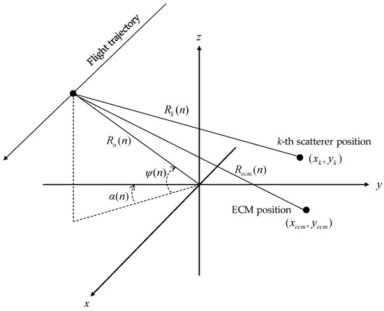
Figure 1.
Geometry of spotlight SAR.
2.1. Reflected Echo Signal
In this subsection, the methodology used to generate reflected echo signals is described. First, the derivation of the reflected echo signal model is presented with detailed descriptions of how to compute the signal with the given reflectivity map. Then, the method used to generate the reflectivity map, which is the input of the reflected echo signal generation, is described.
2.1.1. Derivation of the Reflected Echo Signal Model
The pulses transmitted from the SAR antenna are written as:
where and represent the time and center frequency, respectively, and . represents the baseband signal, with the arbitrary types of the pulse modulation for the -th pulse and fast time , which is defined as:
where is the pulse repetition interval (PRI). Then, the received signal with respect to the geometrical information in Figure 1 can be written as:
where is the speed of light and is the distance from the -th antenna position to the -th scatterer. represents the reflectivity of the -th scatterer, which is an element of the given reflectivity map. The demodulated signal of Equation (3) is represented as:
where is the distance from the -th antenna position to the scene center of spotlight mode SAR, and is the fast time, defined as:
The baseband signal in Equation (4) can be rewritten as:
where is the “reference signal,” defined as:
which is the same as the demodulated signal reflected from the scene center with an amplitude of 1, and is the “scene model,” defined as:
Equation (6) demonstrates that the demodulated echo signal can be obtained by convoluting the reference signal with the scene model , which can be easily conducted in the frequency domain. Additionally, Equations (7) and (8) show that the effects of the baseband signal and the reflectivity are isolated from one another in the reference signal and the scene model, respectively, so that can be calculated without taking into account the pulse modulation that varies from pulse to pulse. The Fourier transform (FT) of Equation (6) leads to the following equation:
where and are the FT of the reference signal and scene model, respectively, which are written as:
where
and is the FT of . The approximation of for is:
where and are the azimuth and grazing angle, respectively. By substituting Equation (13) into (11) and replacing with , where denotes the coordinate of the -th scatterer, the scene model is expressed by:
where and are the spatial frequency, defined as:
and is the two-dimensional spatial FT of , which means that we can obtain the FT of the scene model from the 2D discrete Fourier transform (DFT) of the reflectivity map. However, as represented in (15) and (16), the grid points of the spatial frequency are in a polar grid rather than a rectangular grid, which makes it insufficient to obtain the scene model through the direct fast Fourier transform (FFT) of the reflectivity map. From Equation (14) to Equation (16), the relationship between and can be rewritten as:
where is an operator of the FFT, and is a polar reformatting operator for converting the polar grid data to the rectangular grid, which is usually performed by the interpolation of the data. Thus, can be obtained by the inverse polar reformatting process of , i.e.:
From Equation (18), we can obtain , which is the same as . Then, the FT of the reflected echo is obtained from Equation (9). Finally, the received echo in the pulse and fast time domain is achieved through the inverse fast Fourier transform (IFFT).
2.1.2. Generation of the Reflectivity Map
A distinguishing feature of the SAR images compared to optical images is the presence of noise-like speckles. Several studies have shown that the intensity of the speckled SAR image can be modeled through the elementwise product of the noise model and the intensity of the noise-free image [54,55]. Thus, the speckled complex reflectivity map can be represented as:
The noise model for the intensity has an exponential distribution [54,55], which is represented as:
We used the grayscale optical images as for the proposed simulator.
2.2. Jamming Signal
Similar to the method used to generate the reflected echo signal described above, the generation of the jamming signal based on DRFM repeat jamming is represented in this subsection. The mathematical form of the jamming signal is derived from the spotlight SAR perspective. Then, the typical jamming model suitable for the derived jamming signal equation is presented. Finally, JESZ, which is a measure that represents the reflectivity equivalent to the non-coherent jamming signal, is derived to determine the ERP of the jammer with a given constant SAR transmit power.
2.2.1. Received Jamming Signal Model
The pulses received from ECM antenna are written as:
where is the distance from the -th antenna position to the ECM position. The transmit jamming signal based on the DRFM repeat jamming manner is generated by convolving the jamming model with the replica in Equation (21), which allows the jamming signal to be compressed by the SAR matched filter to achieve a signal processing gain in the range direction. Although DRFM repeat jamming is still an effective jamming method, the entire data of each pulse are required for efficient convolution and sophisticated phase adjustment in the frequency domain, which forces the jammer to use the baseband signal of the previous PRI as the replica. In addition, in order to create false targets or images ahead of the ECM position, the jamming signal must be transmitted before the next SAR transmit signal is received from the ECM antenna, which is another reason why the modulation of the previous pulse should be used as that of the replica. Thus, the transmit jamming signal is represented as:
where is defined as:
and represents the jamming model. Then, the demodulated jamming signal received from the SAR antenna is:
The FT of Equation (24) leads to the following equation:
where and are the FTs of and , respectively, and is defined as:
The demodulated jamming signal generation is achieved through the IFFT of Equation (25). The jamming effect on the SAR image is determined by the jamming model. The jamming models used for the above derived spotlight SAR jamming equations to achieve well-known typical jamming methods are as follows:
- Noise convolution jamming (NCJ): NCJ is a type of barrage jamming used to blanket a specific area in the range direction [42,43]. The jamming model for NCJ is represented as:
- 2.
- False target jamming (FTJ): FTJ is a type of deceptive jamming used to generate the false targets in an arbitrary position in SAR images [46,47,48,49,50]. To generate the false targets, the received jamming signal should have a similar form to the signals reflected from real scatterers, which can be achieved through the following equation:
In Equation (26), is the reflectivity of the -th false target, and is the distance from the -th antenna position to the -th false target. Equation (28) is derived from Equations (9), (11) and (12) by replacing , , and with , , and , respectively. Then, in (25) derived by comparing Equations (25) and (28) is:
Although the jamming model in Equation (29) is quite similar to the scene model in Equation (11), the inverse processing performed to obtain the scene model is not applicable to the jamming model. The reason is that, in order to perform the inverse processing, the ECM should have the information of the SAR antenna position for all pulses in advance of the start of the mission, which is impossible for airborne SAR. Even though there are several methods for the efficient calculation of the jamming model for FTJ [46,47,48,49,50], most of them are based on space-borne SAR, whose mission trajectories are easily estimated. Hence, the jamming model for our proposed simulator is obtained by the direct computation of Equation (29), which increases the computation burden as the number of false targets increases.
2.2.2. Jamming Equivalent Sigma Zero
The power of the reflected target signal received from the SAR antenna is written as:
where is the transmit signal power, is the antenna gain, is the effective area of the receiving antenna, is the RCS of the target, is the slant range from the target to the antenna, and and are the radar transmission loss and 2-way atmospheric loss, respectively. Similarly, the received power of the jamming signal is represented as:
where and are the transmit jamming signal power and antenna gain of the ECM, respectively, is the ECM transmission loss, and denotes the ERP, defined as:
Then, the signal-to-jamming ratio (SJR) at the receiving antenna is derived as:
Due to pulse compression and coherent pulse integration, the SJR in the SAR image achieves the processing gain in the range and azimuth directions, which is written as:
where and are the range and azimuth processing gains, respectively, is the pulse width, is the bandwidth of the signal, is the pulse repetition frequency (PRF), is the wavelength, is the azimuth resolution, and is the aircraft horizontal velocity orthogonal to the target direction. For simplicity, the broadening factors and signal processing losses are omitted in Equation (34). Consequently, the SJR for the image is represented as:
where and are the target reflectivity and grazing angle, respectively, and is the average power, represented as:
Equation (35) is derived through the substitution of the following equations:
Similar to the NESZ, the proposed JESZ is defined as the jamming equivalent reflectivity, which is represented as:
The physical meaning of (i.e., JESZ) in (38) is that, if the received SAR signal contains the non-coherent jamming signal with the ERP of , the targets with a reflectivity lower than will be indistinguishable from the noise-like images generated by the jamming signal. Since the proposed JESZ is independent from the scene or targets, it is an appropriate measure for quantifying the relative performance of the non-coherent jamming on SAR. Moreover, the JESZ is the lower limit of the jamming performance, because the non-coherent jamming is the most power-consuming method for SAR jamming. Therefore, the JESZ can be used as a design requirement so that the ECCM SAR and SAR jammer systems have low and high JESZ, respectively. In our proposed simulator, the JESZ and SAR transmit power are the simulation inputs used to compute the ERP of the jammer through the following equation, derived from Equation (38):
2.3. Signal Received from SAR Antenna
The received signal from the SAR antenna is the sum of the reflected echo signal and the jamming signal, i.e.:
is obtained from Equations (30) and (37), if we set to 1, which makes the power reflected from the maximum point of the given reflectivity map . is obtained from Equations (31) and (39) with the given . It is noted that should be normalized before evaluating Equation (40). This is because in Equation (31) represents the total received jamming signal power, whereas in Equation (30) represents the power received from a single target. Equation (40) is the final form of the SAR raw data in the frequency domain. Although the time domain data are available through the FFT of Equation (40), the form in Equation (40) is directly used in the SAR signal processing in our simulator to perform the pulse compression in the frequency domain.
3. Signal Processing
In this section, we briefly introduce the signal processing for spotlight SAR and its mathematical descriptions to explain the structure of the proposed SAR simulator. The SAR signal processing in the simulator is divided into two parts: the pulse compression and image formation. The pulse compression is performed each time a signal is received from the SAR antenna, which is achieved through matched filtering with motion compensation. After all the received pulses are compressed, the image formation is achieved through polar reformatting, 2-D IFFT, and autofocus.
3.1. Pulse Compression
Pulse compression is achieved through the matched filtering of Equation (40), and the matched filter is designed to extract , which is equal to the 2D FT of the reflectivity map . Thus, the desired matched filter is written as:
where denotes the complex conjugate. The exponential term in Equation (41) represents the motion compensation with respect to the scene center. Equation (41) represents the ideal matched filter without motion errors, whereas motion errors always exist in real airborne SAR system. Therefore, the motion errors should be considered to the motion compensation term in the matched filter for the appropriate modeling of the real systems. The estimated matched filter with motion error is represented as:
where and are the estimates of and , respectively. is usually obtained from the appropriate post-processing of the navigation data, often referred to as the motion measurements [56]. Although there are various motion compensation methods [56,57,58,59], a simple velocity integration method, which estimates the current platform position by integrating the velocity at the first position of the SAR mission, is used in our simulator to attenuate the high frequency motion errors. The estimated distance obtained from the velocity integration method is represented as:
where denotes the l2-norm. is the -th estimated antenna position, and is the position of the scene center. and are expressed in an arbitrary Cartesian coordinate system, e.g., the earth-centered earth-fixed (ECEF) coordinate. estimated by the velocity integration is expressed as:
where and denote the position for the 1st pulse and the antenna velocity for the -th position, respectively, measured by the navigation sensors. The coordinate system of and is the same as that of . and can be generated by adding the navigation errors to the true position and velocity. With computed from Equations (43) and (44), the compressed signal is derived as:
where is the motion error, defined as:
The first and second terms in Equation (45) represent the matched filter outputs for the reflected echo signal and jamming signal, respectively. The impulse responses of the outputs are determined from the inverse Fourier transform (IFT) of and . It is clear that the former result is a sinc function with a resolution determined by the bandwidth of the signal . If we assume that the satisfies the pulse diversity, i.e., all the baseband transmit signals are orthogonal to one another, the latter shows a noise-like signal because the signal power will be spread to all the time domains in the pulse width. Thus, we can expect that the jamming effect is rejected in the output of the simulator if the pulse diversity is applied to all the baseband signals and the jamming power is sufficiently small. As described in the previous section, however, the targets with a reflectivity of less than the JESZ would be overshadowed by the noise-like images from the non-coherent jamming signal, which is the reason why the JESZ should be considered in the design of the ECCM SAR.
3.2. Image Formation
For simplicity, if we assume that for all and , the pulse compression result of the reflected echo signal, i.e., the first term in Equation (45), is the FT of the scene model, whose phase is corrupted due to the motion error. As we can see in Equations (14) and (17), the image formation is achieved through the polar reformatting and 2D IFFT, as the following equation:
where is the resultant image, whose quality is degraded due to the motion error, and denotes the 2D IFFT. The term related to the jamming signal is omitted in Equation (47). The phase-corrupted image can be restored by the phase error correction through the autofocus algorithm.
4. Simulator Structure and Simulation Results
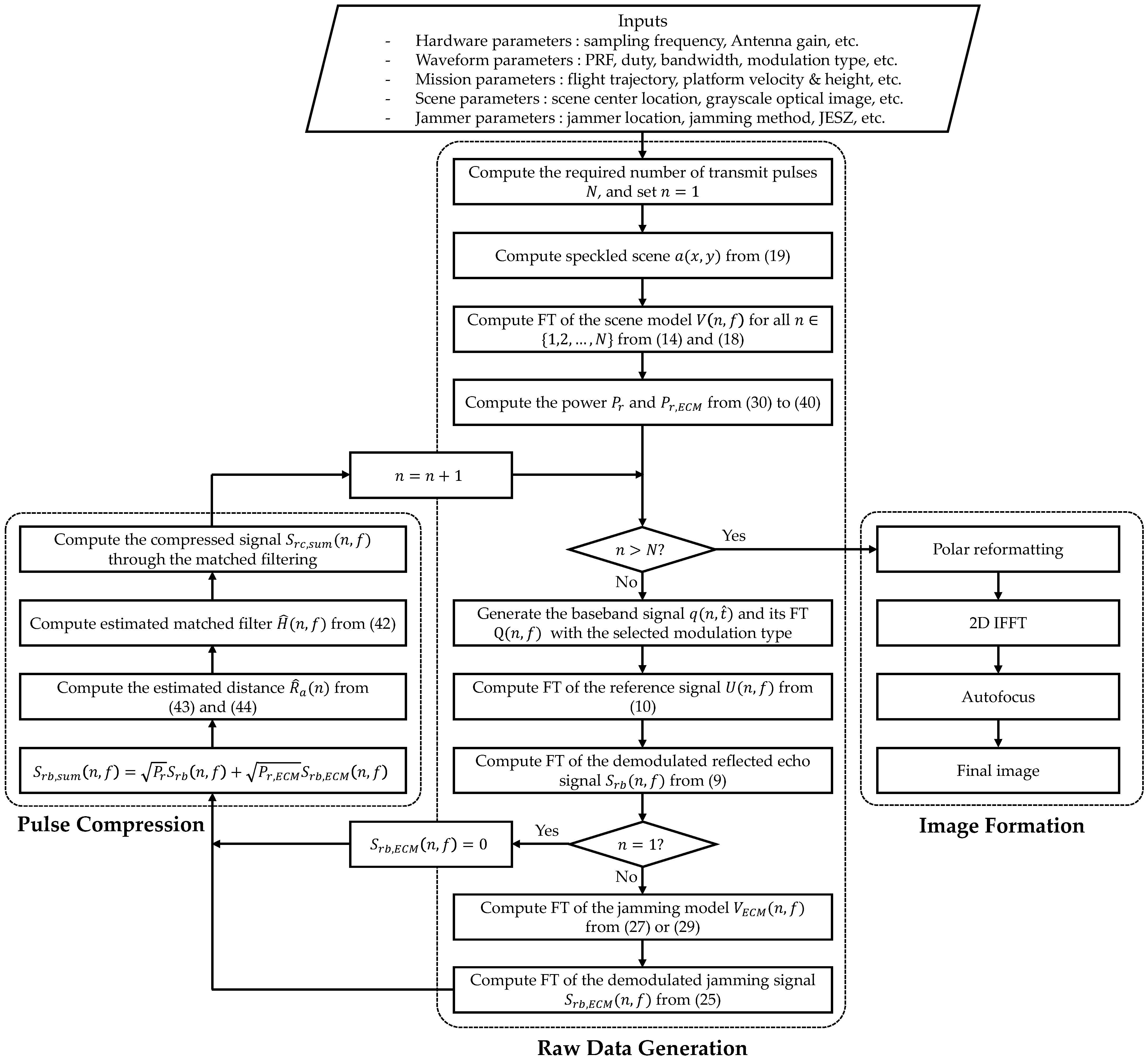
In this section, detailed descriptions of the structure and methodology of the proposed airborne spotlight SAR simulator are presented with the simulation results. The flowchart of the simulator is shown in Figure 2.
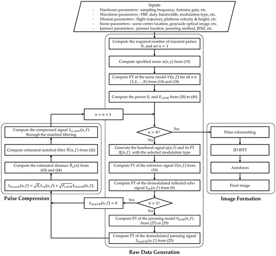
Figure 2.
Flowchart of the proposed airborne spotlight SAR simulator.
4.1. Inputs for the Simulator
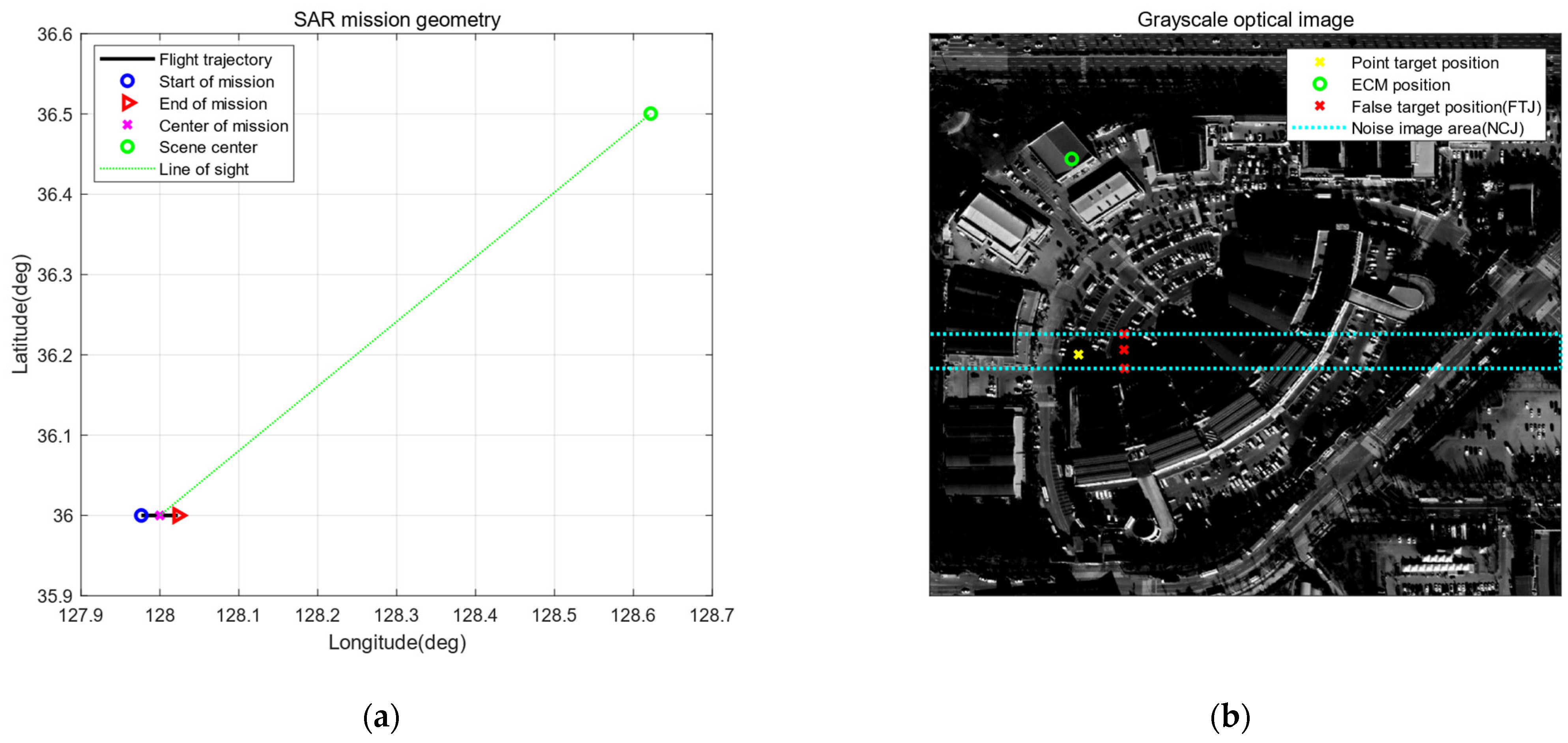
The simulation starts with the required inputs, such as the hardware parameters, waveform parameters, mission parameters, flight trajectory, position of the scene center, ECM, false target/image, etc. Table 1 and Figure 3 show examples of the inputs for the simulation used to obtain all the simulation results for the rest of this paper. All the parameters were set to achieve a resolution finer than 0.5 m. The navigation errors in Table 1 were applied to the simulator to demonstrate the motion measurement and autofocus. We assumed that the navigation errors have a normal distribution. The flight trajectory and scene center position in Figure 3a was determined to obtain the slant range and squint angle in Table 1. The grayscale optical image used to generate the reflectivity map is shown in Figure 3b. The positions of the point target, ECM, false targets, and the area of the noise image are also represented in that figure. The point target was inserted to the scene to verify the final image quality with the impulse response function (IRF).

Table 1.
Input parameters of the proposed airborne SAR simulator.
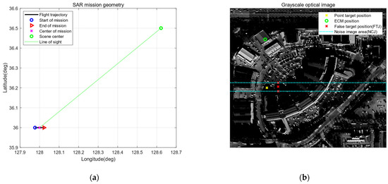
Figure 3.
Graphical representations of the inputs for the proposed airborne SAR simulator. (a) SAR mission geometry, including flight trajectory, flight direction, and scene center. (b) Grayscale optical image used to generate the reflectivity map, and the positions of the point target, ECM, false targets, and the area of false image due to jamming signal.
4.2. Raw Data Generation and Pulse Compression
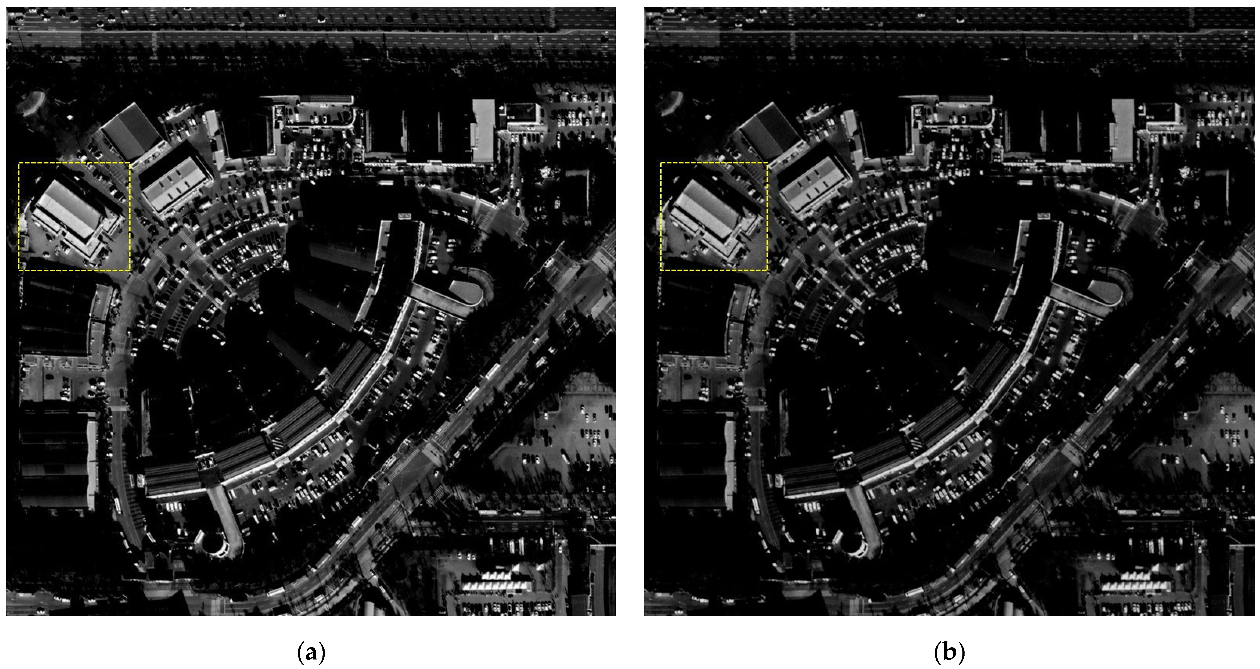
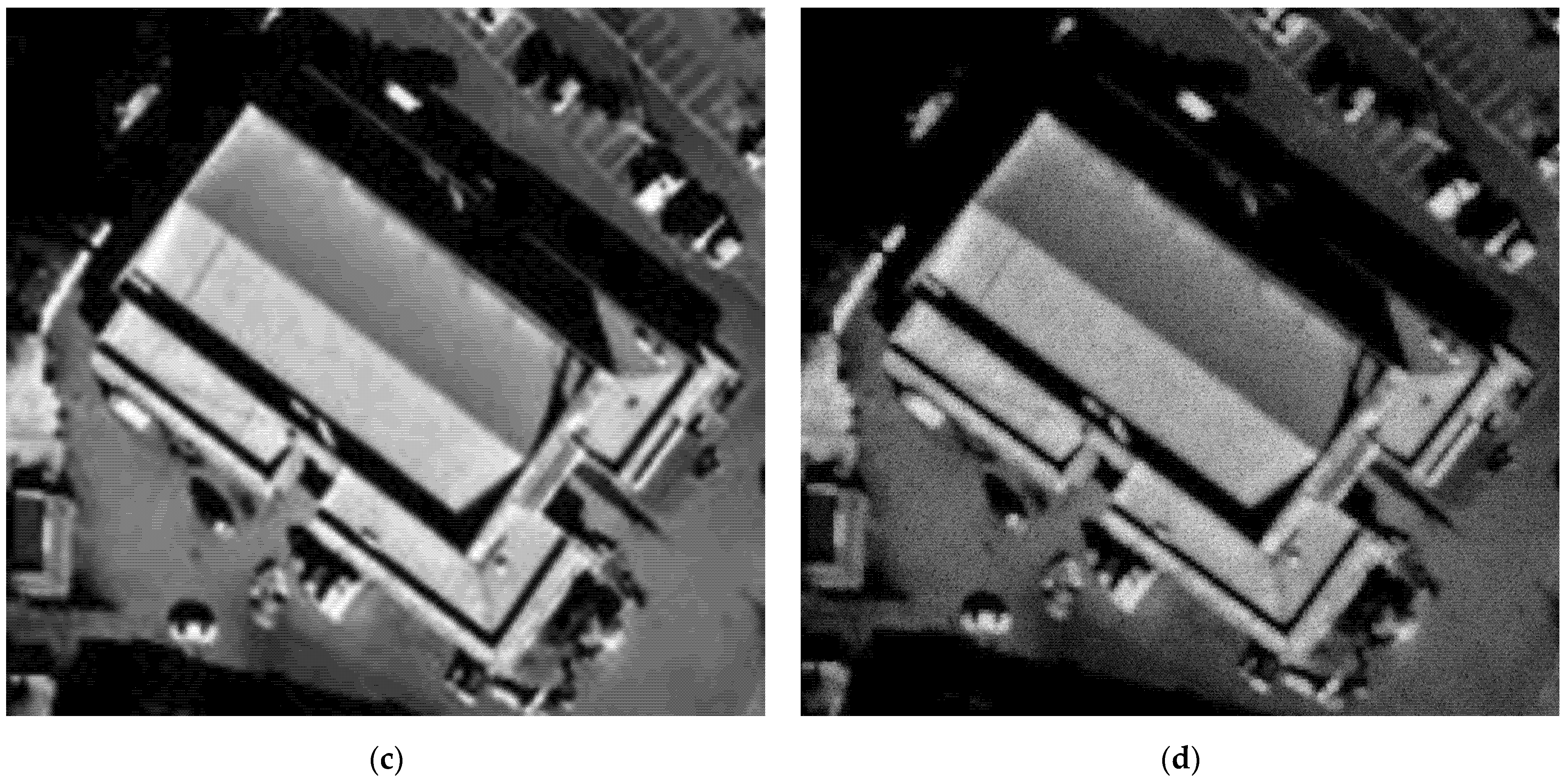
The raw data generation process starts with the initialization stage. In this process, the required number of transmit pulses is firstly computed from PRF and SAT. Then, the speckled scene is computed from Equation (19). The scenes with and without speckles are shown in Figure 4a,b, respectively. The effect of the speckle application can be confirmed by the images in Figure 4c,d, which are the enlarged images of the yellow boxes in Figure 4a,b, respectively. With the speckled image in Figure 4b, the FT of the scene model is computed from Equations (14) and (18). Since the number of azimuth pixels in will be different with respect to the required number of pulses, they should be matched by zero-padding or appropriate filtering when computing Equation (18). The number of samples in a pulse should also be matched by the same process. After is computed, the power of the received reflected echo and jamming signal is computed from Equations (30) to (40), which is the last procedure of the initialization stage.
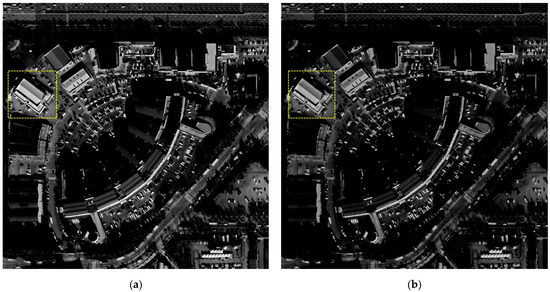
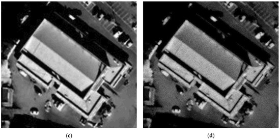
Figure 4.
Grayscale images to simulate SAR raw data. (a) Grayscale image without speckle. (b) Grayscale image with speckle generated from (19). (c) Enlarged image of the yellow box in (a). (d) Enlarged image of the yellow box in (b).
After the initialization is completed, the simulator starts generating the raw data. The first step is to generate the baseband signal for the current pulse number and its FT with the selected modulation type. If the pulse diversity is applied to the waveform design, this step should be repeated for all the pulses. Meanwhile, if the baseband signal for all transmit pulses are the same, this step only needs to be performed once the first time. Next, the FT of the reference signal is computed from (10), with obtained from the previous step. With and obtained from the initialization stage, the FT of the demodulated reflected echo signal is computed from Equation (9).
After the reflected echo signal is computed, it initiates the jamming signal generation unless the current pulse is the first transmit pulse. The FT of the jamming model for the NCJ or FTJ is computed from Equations (27) or (29), respectively. Then, the FT of the demodulated jamming signal is computed from Equation (25). As previously described, should be normalized before computing , so that represents the FT of the received jamming signal with the unit power. This is the final step in the raw data generation for the current pulse number.
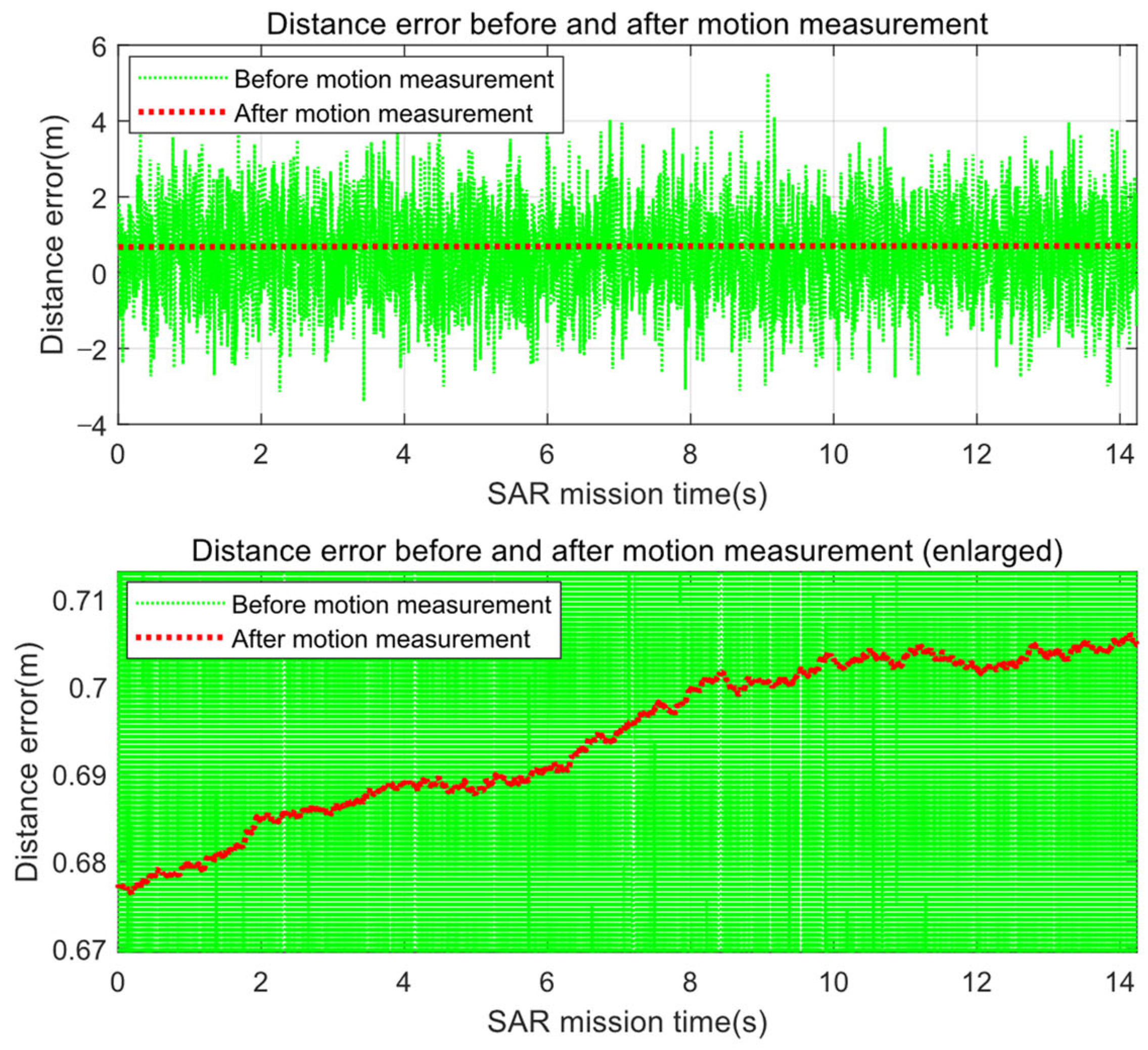
In our proposed simulator, the pulse compression is performed as soon as the raw data for the current pulse are generated, which enables the reduction of the unnecessary memory used to store the replicas that vary from pulse to pulse. Firstly, the received signal is computed from Equation (40) with the previously calculated , , , and . Then, the estimated distance in Equation (42) is computed by the motion measurement process represented in Equations (43) and (44). The distance errors before and after the motion measurement, i.e., the velocity integration, is represented in Figure 5. The residual errors in Figure 5 will be compensated by the autofocus algorithm.
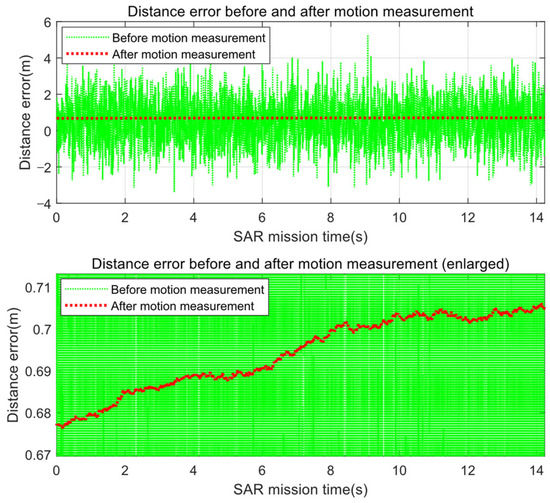
Figure 5.
Errors of the distance from the SAR antenna to the scene center before/after the motion measurement, i.e., the velocity integration. The lower figure is an enlarged view of the upper figure.
After the motion measurement is completed, the estimated matched filter is computed from Equation (42) with the estimated distance . Then, the matched filtering of the signal is performed, which is the last step of the pulse compression. Except for the initialization stage, the raw data generation and pulse compression processes are repeated until compressed pulses are generated.
4.3. Image Formation
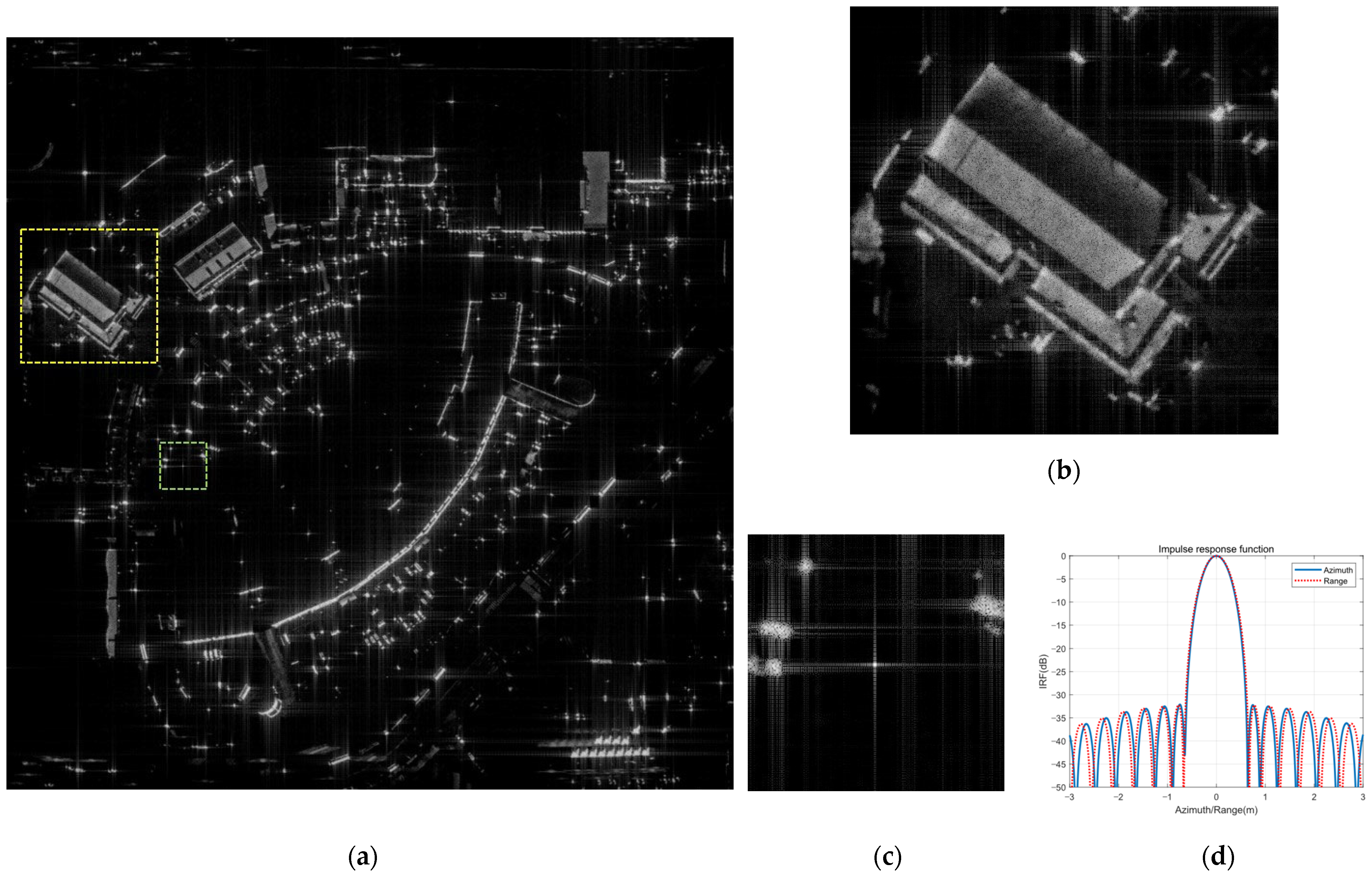
As previously described, the image formation is achieved through the polar reformatting and 2D IFFT of the compressed signal generated from the raw data generation and pulse compression process. A 2D Taylor window with a peak side-lobe level of −32 dB is applied before the 2D IFFT. The residual phase errors due to the motion measurement errors are compensated by the autofocus algorithm. The image formation results without the motion measurement errors and jamming signals are shown in Figure 6. Figure 6a–c show that the image and point target are well-focused, and Figure 6d demonstrates that the resolutions of the azimuth and range satisfy the design goal (0.5 m). The simulation results for the autofocus and pulse diversity with the motion errors and jamming signals are demonstrated and compared with the results in Figure 6, as follows.
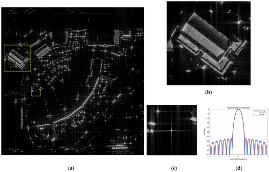
Figure 6.
The image formation results without the motion measurement errors and jamming signal. (a) Full size image. (b) Enlarged image of the yellow box. (c) Enlarged image of the green box near the point target. (d) IRF of the point target.
4.3.1. Images with Motion Measurement Errors
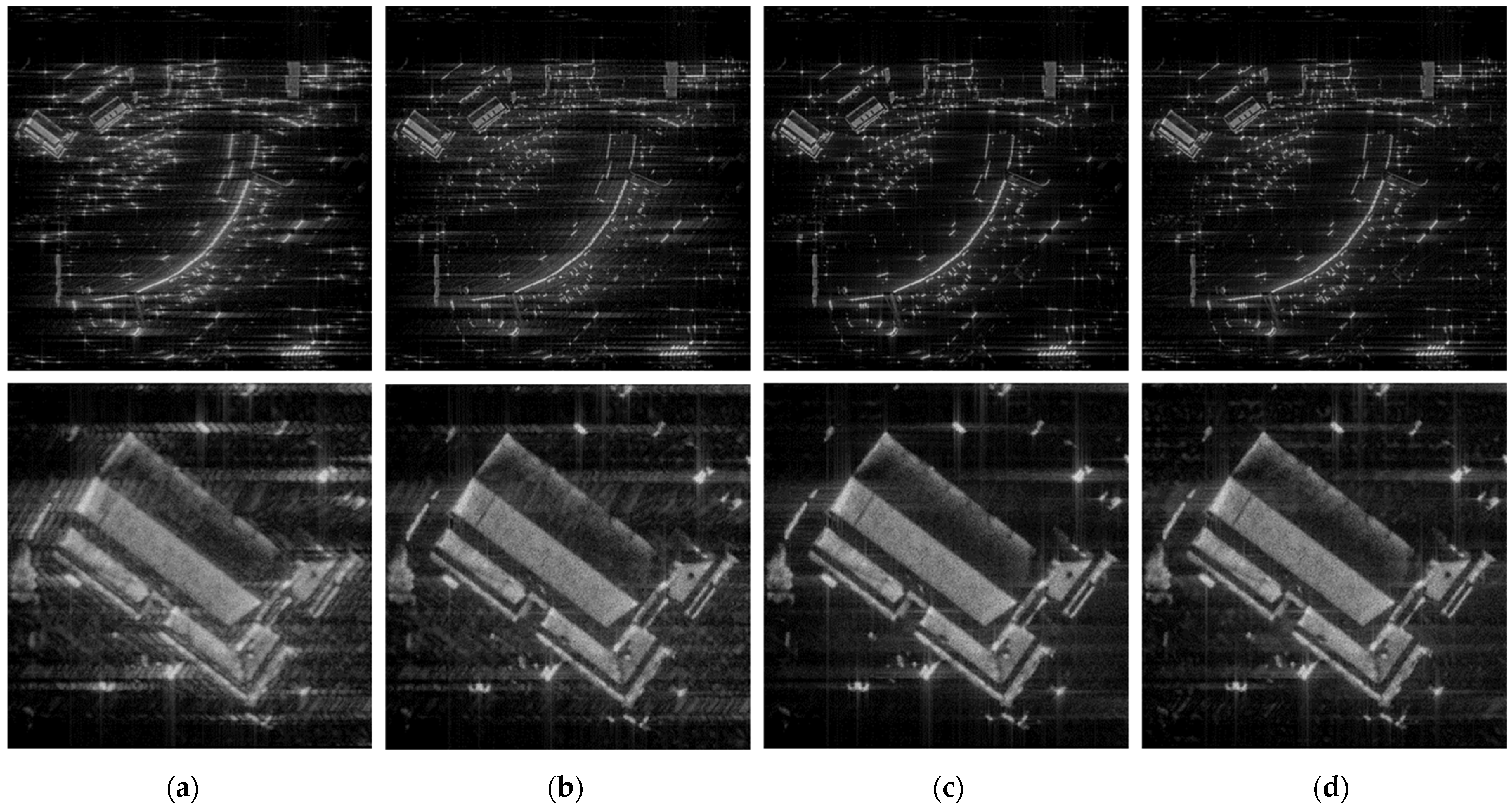
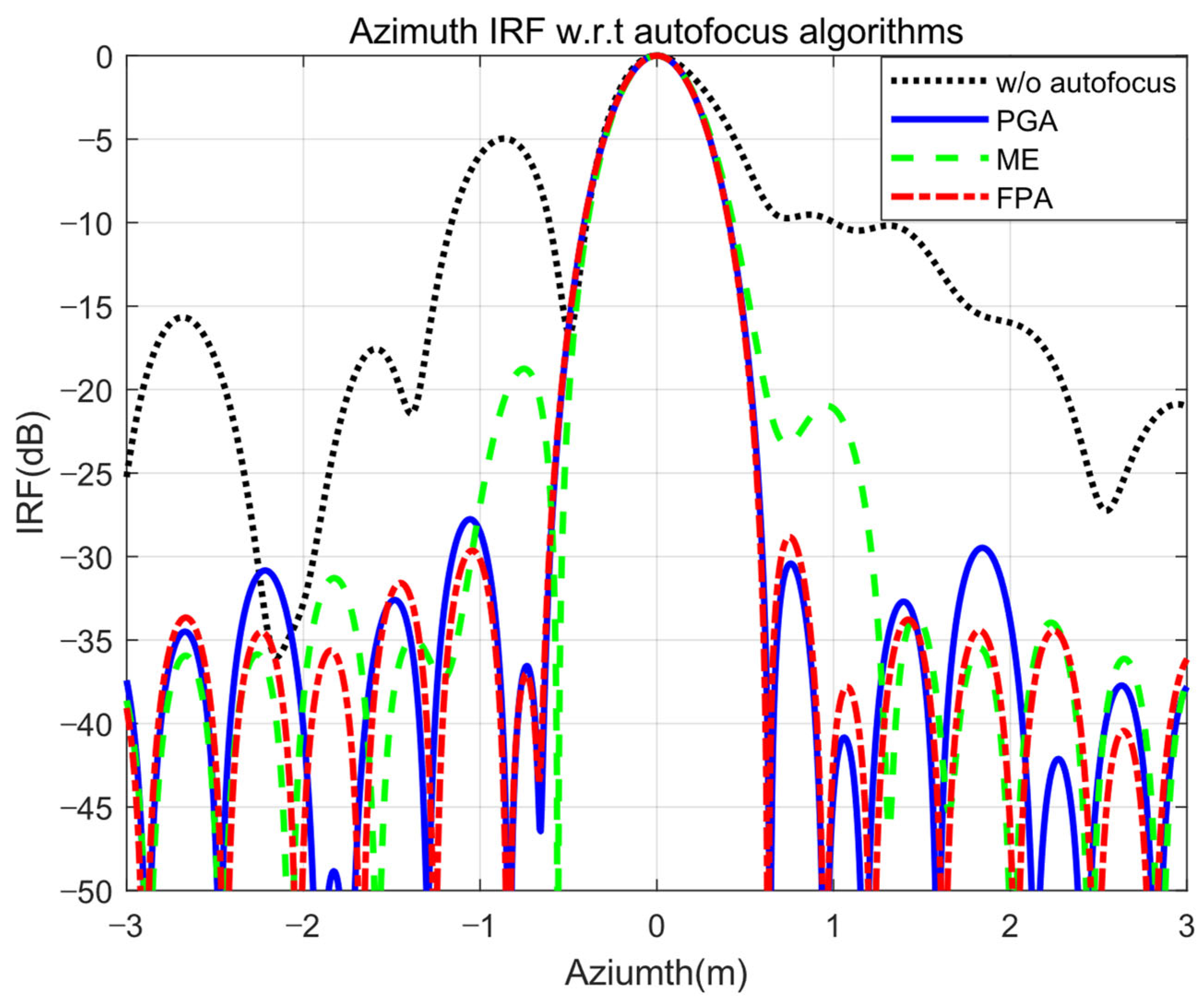
The image formation results with the motion measurement errors represented in Figure 5 are shown in Figure 7. The image without autofocus in Figure 7a shows the degradation of the image quality compared with the image in Figure 6a,b, from which it can be inferred that the motion measurement errors are appropriately applied to the proposed simulator. Figure 7b–d represent the images with PGA, ME, and FPA, respectively, and the corresponding IRF and quantitative image qualities are represented in Figure 8 and Table 2. For all the autofocus algorithms, the iteration stopped when the image variation relative to the previous image was less than 10−4, which is the same condition represented in [29]. The results demonstrate that PGA shows better IRF performance aspects, such as resolution, peak to side-lobe ratio (PSLR), and integrated side-lobe ratio (ISLR), than those of ME, while ME shows better contrast and entropy performances than PGA. FPA shows moderate IRF, contrast, and entropy performance with an appropriate number of iterations. All these trends are mostly consistent with the autofocus performance trends confirmed in [29], based on real data from actual flight tests, which indicates that the raw data generated by the proposed simulator closely simulate the real data with the motion measurement errors. Thus, it is verified through the simulation results that the proposed simulator is well-designed for simulating SAR raw data, including motion errors, which confirms that it is an appropriate simulator for verifying various autofocus algorithms for airborne SAR systems.
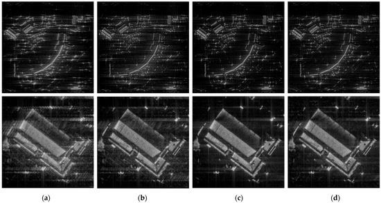
Figure 7.
The image formation results with the motion measurement errors. The images in the upper and bottom row represent the full-size images and enlarged images of the same area in Figure 6b, respectively. The images in each column are produced (a) without autofocus, (b) with PGA, (c) with ME, and (d) with FPA.
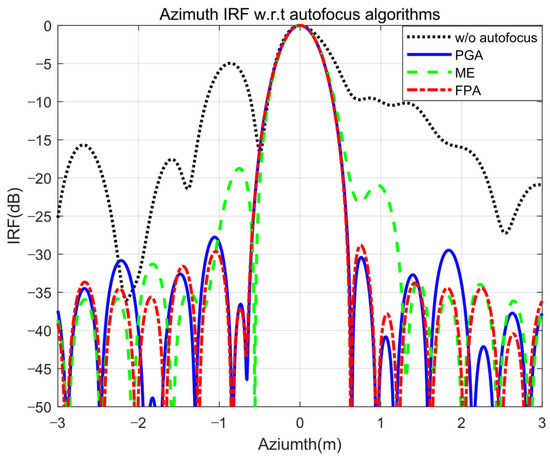
Figure 8.
IRF measured from the inserted point target for each of the autofocus algorithms.
Table 2.
Comparison of the image qualities of different autofocus algorithms.
4.3.2. Images with the Jamming Signals
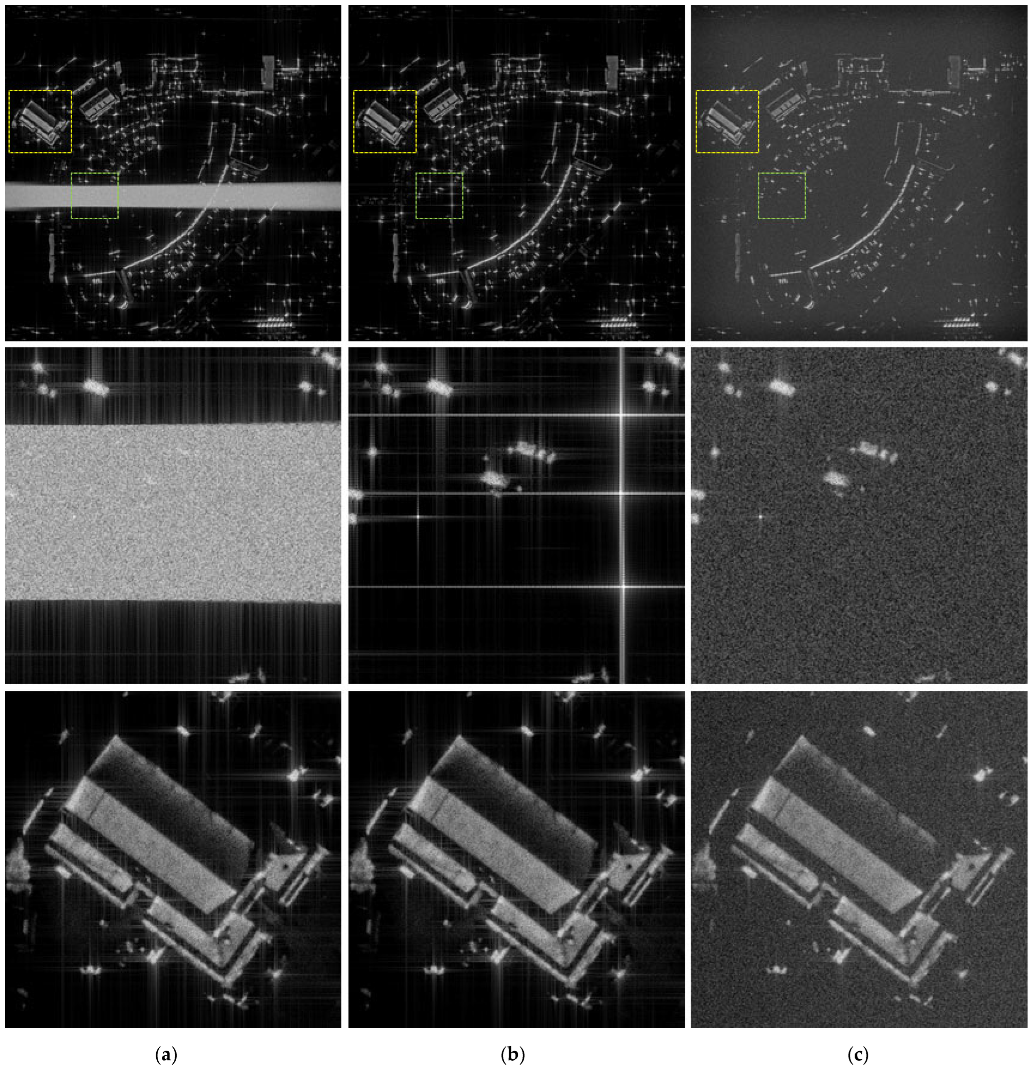
The image formation results with the jamming signals are represented in Figure 9. As previously described in Section 3, the image with NCJ in Figure 9a shows the blanket effect at the specific area in the range direction marked in Figure 3b. Likewise, false targets are generated through FTJ at the marked point in Figure 3b, as shown in Figure 9b. These typical repeating jamming methods are countered by the pulse diversity scheme implemented in the proposed simulator. The image formation results shown in Figure 9c demonstrate that the blanket effect and false targets are removed by the pulse diversity scheme. However, the pulse diversity scheme only prevents the jamming signal from being compressed; it does not completely eliminate the jamming signal. Thus, the jamming power is spread to all the areas of the image, unlike the jamming power of the NCJ and FTJ, which is concentrated in specific areas or points of the image. These properties are represented in Figure 9.
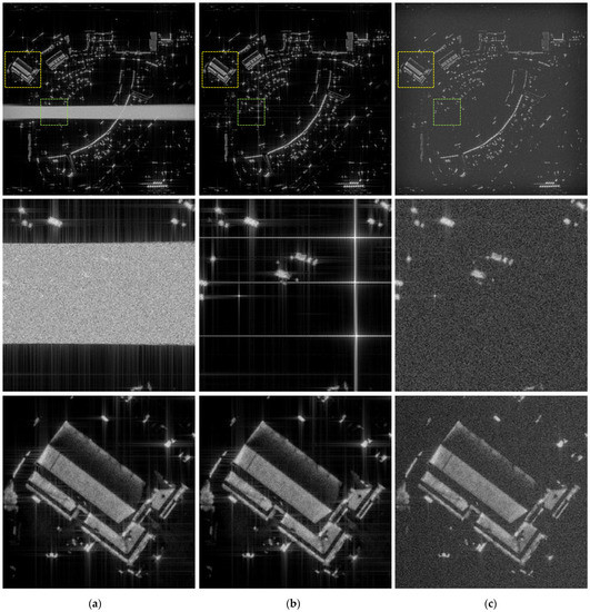
Figure 9.
The image formation results with the jamming signals. The images in the first row show the full-size images. The images in the second and third row represents the enlarged images of the yellow and green boxes in the images of the first row, respectively. The images in (a,b) show the jamming results of the NCJ and FTJ, respectively, and those in (c) show the images with pulse diversity.
As previously described, the jamming effect of the pulse diversity scheme is the same as that of non-coherent jamming. Thus, even if the pulse diversity scheme is applied, the target with a reflectivity of less than JESZ is not visible in the image. The value of the desired JESZ, in order to determine the ERP of the jammer, is set to −20 dB for the simulation. Therefore, we can expect that the target with a reflectivity of less than −20 dB is indistinguishable from the noise-like jamming effect. The simulation results with different values of the point target reflectivity are shown in Figure 10, and the corresponding quantitative results are represented in Table 3. As shown in Figure 10, it is difficult to distinguish the point target from the noise-like jamming effect as the reflectivity decreases, and the point target finally disappears at the reflectivity of −20 dB, equal to the desired JESZ. Table 3 shows the measured JESZ from the images in Figure 10, and it can be confirmed that the ERP of the jammer is correctly calculated by the simulator to obtain the desired JESZ of −20 dB.
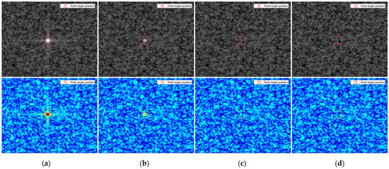
Figure 10.
The images enlarged near the inserted point targets. The images in the bottom row represent the upsampled images of the images in the upper row. The values of the point target reflectivity are set to (a) 30 dB, (b) 10 dB, (c) −10 dB, and (d) −20 dB.
Table 3.
Measured SJR and JESZ with differing reflectivity of the point target.
4.3.3. Discussion of the Simulation Results concerning the JESZ
The simulation results concerning the JESZ demonstrate that the proposed JESZ can be used as a quantitative requirement for designing the power of the ECCM SAR systems or SAR jamming systems. The conventional SAR systems require sufficiently high transmit power to obtain high-quality images, and the power is usually determined from the NESZ. In the case of ECCM SAR systems, the non-coherent jamming effect due to the pulse diversity scheme is the same as the effect of the received signal noise. Hence, the JESZ with advance information of the jamming power should be a requirement for designing ECCM SAR systems to overcome the noise-like jamming effect due to the jamming signals and pulse diversity. Similarly, from the point of view of the jammer, the transmit power of the SAR jamming systems should also be sufficiently high to overshadow the specific targets in the image through the non-coherent jamming effect, because ECCM SAR systems can counter the coherent repeating jamming method through pulse diversity. Thus, the JESZ with advance knowledge of the ECCM SAR signal power should also be a requirement for the design of SAR jamming systems. Therefore, we can conclude that the proposed simulator can not only be used to verify the methods of ECCM SAR or SAR jamming, but it is also useful for ECCM SAR or SAR jamming system design.
5. Conclusions
In this paper, we proposed a simulator which includes most of the required features, such as the motion measurement errors, pulse diversity, and SAR jamming signals, to verify the performance of the airborne spotlight ECCM SAR. The models for received reflected echo and jamming signal are derived in consideration of the spotlight geometry and pulse diversity. We proposed a new measure, called JESZ, to design ECCM SAR or SAR jamming systems, and the proposed simulator uses the JESZ to determine the ERP of the jammer. The motion compensation errors are also considered in the simulator design by the addition of the navigation sensor errors in the motion measurement process. In order to demonstrate the validity and usefulness of the proposed simulator, simulations for autofocus, SAR jamming, and ECCM SAR with pulse diversity were performed. The autofocus simulation results show that the performance trends of various autofocus algorithms were found to be similar to those of actual flight tests data. The simulation results of SAR jamming and SAR ECCM with pulse diversity indicate that the proposed JESZ is well-defined measure for quantifying the power requirements of ECCM SAR and SAR jammers.
Author Contributions
Conceptualization, H.L.; investigation, K.-W.K.; methodology, H.L.; supervision, K.-W.K.; validation; H.L.; writing—original draft, H.L.; writing—review & editing, K.-W.K. All authors have read and agreed to the published version of the manuscript.
Funding
This research received no external funding.
Conflicts of Interest
The authors declare no conflict of interest.
References
- Carrara, W.G.; Goodman, R.S.; Majewski, R.M. Spotlight Synthetic Aperture Radar: Signal Processing Algorithms; Artech House: Norwood, MA, USA, 1995. [Google Scholar]
- Jansing, E.D. Introduction to Synthetic Aperture Radar: Concepts and Practice; McGraw-Hill Education: New York, NY, USA, 2021. [Google Scholar]
- Oliver, C.; Quegan, S. Understanding Synthetic Aperture Radar Images; SciTech Publishing: Noida, India, 2004. [Google Scholar]
- Franceschetti, G.; Iodice, A.; Migliaccio, M.; Riccio, D. A novel across-track SAR interferometry simulator. IEEE Trans. Geosci. Remote Sens. 1998, 36, 950–962. [Google Scholar] [CrossRef]
- Zhang, F.; Hu, C.; Li, W.; Hu, W.; Wang, P.; Li, H. A Deep Collaborative Computing Based SAR Raw Data Simulation on Multiple CPU/GPU Platform. IEEE J. Sel. Top. Appl. Earth Obs. Remote Sens. 2017, 10, 387–399. [Google Scholar] [CrossRef]
- Zhang, F.; Yao, X.; Tang, H.; Yin, Q.; Hu, Y.; Lei, B. Multiple Mode SAR Raw Data Simulation and Parallel Acceleration for Gaofen-3 Mission. IEEE J. Sel. Top. Appl. Earth Obs. Remote Sens. 2018, 11, 2115–2126. [Google Scholar] [CrossRef]
- Zhang, F.; Hu, C.; Li, W.; Hu, W.; Wang, P. Accelerating Time-Domain SAR Raw Data Simulation for Large Areas Using Multi-GPUs. IEEE J. Sel. Top. Appl. Earth Obs. Remote Sens. 2014, 7, 3956–3966. [Google Scholar] [CrossRef]
- Li, Z.X.; Su, D.D.; Zhu, H.J.; Li, W.; Zhang, F.; Li, R.R. A fast synthetic aperture radar raw data simulation using cloud computing. Sensors 2017, 17, 113. [Google Scholar] [CrossRef]
- Rahmanizadeh, A.; Amini, J. An integrated method for simulation of synthetic aperture radar (SAR) raw data in moving target detection. Remote Sens. 2017, 9, 1009. [Google Scholar] [CrossRef]
- Guo, Z.; Fu, Z.; Chang, J.; Wu, L.; Li, N. A Novel High-Squint Spotlight SAR Raw Data Simulation Scheme in 2-D Frequency Domain. Remote Sens. 2022, 14, 651. [Google Scholar] [CrossRef]
- Franceschetti, G.; Migliaccio, M.; Riccio, D.; Gilda, S. SARAS: A synthetic aperture radar (SAR) raw signal simulator. IEEE Trans. Geosci. Remote Sens. 1992, 30, 110–123. [Google Scholar] [CrossRef]
- Wang, Y.; Zhang, Z.; Deng, Y. Squint spotlight SAR raw signal simulation in the frequency domain using optical principles. IEEE Trans. Geosci. Remote Sens. 2008, 46, 2208–2215. [Google Scholar] [CrossRef]
- Luo, Y.; Song, H.; Wang, R.; Deng, Y.; Zheng, S. An accurate and efficient extended scene simulator for FMCW SAR with static and moving targets. IEEE Geosci. Remote Sens. Lett. 2014, 11, 1672–1676. [Google Scholar]
- Khwaja, A.; Ferro-Famil, L.; Pottier, E. SAR raw data generation using inverse SAR image formation algorithms. In Proceedings of the IEEE International Symposium on Geoscience Remote Sensing, Denver, CO, USA, 31 July 2006. [Google Scholar]
- Khwaja, A.S.; Ferro-Famil, L.; Pottier, E. Efficient SAR raw data generation for anisotropic urban scenes based on inverse processing. IEEE Geosci. Remote Sens. Lett. 2009, 6, 757–761. [Google Scholar] [CrossRef]
- Liu, B.; He, Y. SAR Raw Data Simulation for Ocean Scenes Using Inverse Omega-K Algorithm. IEEE Trans. Geosci. Remote Sens. 2016, 54, 6151–6169. [Google Scholar] [CrossRef]
- Deng, B.; Qing, Y.; Li, H.W.X.; Li, Y. Inverse frequency scaling algorithm (IFSA) for SAR raw data simulation. In Proceedings of the International Conference on Signal Processing Systems (ICSPS), Dalian, China, 5–7 July 2010; pp. 317–320. [Google Scholar]
- Eldhuset, K. High resolution spaceborne INSAR simulation with extended scenes. In Proceedings of the IEE Proceedings-Radar, Sonar and Navigation, Cincinnati, OH, USA, 25 July 2005; Volume 152, pp. 53–57. [Google Scholar]
- Duysak, H.; Yiğit, E. Investigation of the performance of different wavelet-based fusions of SAR and optical images using Sentinel-1 and Sentinel-2 datasets. Int. J. Eng. Geosci. 2022, 7, 81–90. [Google Scholar] [CrossRef]
- Wahl, D.E.; Eichel, P.H.; Ghiglia, D.C.; Jakowatz, C.V. Phase gradient autofocus-A robust tool for high resolution SAR phase correction. IEEE Trans. Aerosp. Electron. Syst. 1994, 30, 827–835. [Google Scholar] [CrossRef]
- Wang, J.; Liu, X. SAR minimum-entropy autofocus using an adaptive-order polynomial model. IEEE Geosci. Remote Sens. Lett. 2006, 3, 512–516. [Google Scholar] [CrossRef]
- Zeng, T.; Wang, R.; Li, F. SAR Image Autofocus Utilizing Minimum-Entropy Criterion. IEEE Geosci. Remote Sens. Lett. 2013, 10, 1552–1556. [Google Scholar] [CrossRef]
- Wang, J.; Liu, X.; Zhou, Z. Minimum-entropy phase adjustment for ISAR. IEEE Proc. Radar Sonar Navig. 2004, 151, 203–209. [Google Scholar] [CrossRef]
- Huang, X.; Ji, K.; Leng, X.; Dong, G.; Xing, X. Refocusing Moving Ship Targets in SAR Images Based on Fast Minimum Entropy Phase Compensation. Sensors 2019, 19, 1154. [Google Scholar] [CrossRef]
- Onhon, N.O.; Cetin, M. A sparsity-driven approach for joint SAR imaging and phase error correction. IEEE Trans. Image Process. 2012, 21, 2075–2088. [Google Scholar] [CrossRef]
- Ugur, S.; Arikan, O. SAR image reconstruction and autofocus by compressed sensing. Digit. Signal Process. 2012, 22, 923–932. [Google Scholar] [CrossRef]
- Kang, M.S.; Kim, K.T. Compressive sensing based SAR imaging and autofocus using improved Tikhonov regularization. IEEE Sens. J. 2019, 19, 5529–5540. [Google Scholar] [CrossRef]
- Zhao, L.; Wang, L.; Bi, G.; Li, S.; Yang, L.; Zhang, H. Structured sparsity-driven autofocus algorithm for high-resolution radar imagery. Signal Proc. 2016, 125, 376–388. [Google Scholar] [CrossRef]
- Lee, H.; Jung, C.S.; Kim, K.W. Feature Preserving Autofocus Algorithm for Phase Error Correction of SAR Images. Sensors 2021, 21, 2370. [Google Scholar] [CrossRef]
- Lang, D.M. Range Sidelobe Response from the Use of Polyphase Signals in Spotlight Synthetic Aperture Radar; Naval Postgraduate School: Monterey, CA, USA, 2015. [Google Scholar]
- Wagner, Z.A. Investigation of Frequency Agility for LPI-SAR Waveforms; Naval Postgraduate School: Monterey, CA, USA, 2018. [Google Scholar]
- Yu, X.; Fu, Y.; Nie, L.; Zhao, G.; Zhang, W. A waveform with low intercept probability for OFDM SAR. In Proceedings of the IEEE Progress in Electromagnetics Research Symposium (PIERS), Shanghai, China, 8–11 August 2016; pp. 2054–2058. [Google Scholar]
- Garmatyuk, D.S.; Narayanan, R.M. ECCM capabilities of an ultrawideband bandlimited random noise imaging radar. IEEE Trans. Aerosp. Electron. Syst. 2002, 28, 1243–1255. [Google Scholar] [CrossRef]
- Tarchi, D.; Lukin, K.; Fortuny-Guasch, J.; Mogyla, A.; Vyplavin, P.; Sieber, A. SAR Imaging with Noise Radar. IEEE Trans. Aerosp. Electron. Syst. 2010, 46, 1214–1225. [Google Scholar] [CrossRef]
- Wei, L.; Lin, Y.; Xu, G. A new method of phase-perturbed LFM chirp signals for SAR ECCM. In Proceedings of the China International SAR Symposium, Shanghai, China, 10–12 October 2018; pp. 1–4. [Google Scholar]
- Hossain, M.A.; Elshafiey, I.; Alkanhal, M.A.; Mabrouk, A. Anti-jamming capabilities of UWB-OFDM SAR. In Proceedings of the 2011 8th European Radar Conference, Manchester, UK, 12–14 October 2011; pp. 313–316. [Google Scholar]
- Feng, X.; Xu, X. ECCM performance analysis of chaotic coded orthogonal frequency division multiplexing (COFDM) SAR. In Proceedings of the SPIE, Orlando, FL, USA, 21 June 2011; pp. 80211K-1–80211K-9. [Google Scholar]
- Chunrui, Y.; Xile, M.; Yongsheng, Z.; Zhen, D.; Diannong, L. Multichannel SAR ECCM based on Fast-time STAP and Pulse diversity. In Proceedings of the IEEE International Geoscience and Remote Sensing Symposium (IGARSS), Vancouver, BC, Canada, 24–29 July 2011; pp. 921–924. [Google Scholar]
- Schuerger, J.; Garmatyuk, D. Multifrequency OFDM SAR in presence of deception jamming. EURASIP J. Adv. Signal Processing 2010, 2010, 451851. [Google Scholar] [CrossRef]
- Sounekh, M. SAR-ECCM using phase-perturbed LFM chirp signals and DRFM repeat jammer penalization. IEEE Trans. Aerosp. Electron. Syst. 2006, 42, 191–204. [Google Scholar] [CrossRef]
- Huang, H.; Zhou, Y.; Jiang, W.; Huang, Z. A new time-delay echo jamming style to SAR. In Proceedings of the 2nd International Conference on Signal Processing Systems, Dalian, China, 5–7 October 2010; Volume 3, pp. V3-14–V3-17. [Google Scholar]
- Bo, L. Simulation study of noise convolution jamming countering to SAR. In Proceedings of the 2010 International Conference on Computer Design and Applications, Qinhuangdao, China, 25–27 June 2010; Volume 4, pp. V4-130–V4-133. [Google Scholar]
- Wei, Y.; Hang, R.; Shuxian, Z.; Li, Y. Study of noise jamming based on convolution modulation to SAR. In Proceedings of the 2010 International Conference on Computer, Mechatronics, Control and Electronic Engineering, Changchun, China, 24–26 August 2010; pp. 169–172. [Google Scholar]
- Ammar, M.; Hassan, H.; Abdel-Latif, M.; Elgamel, S.A. Performance evaluation of SAR in presence of multiplicative noise jamming. In Proceedings of the 2017 34th National Radio Science Conference (NRSC), Alexandria, Egypt, 13–16 March 2017; pp. 213–220. [Google Scholar]
- Chang, X.; Dong, C. A Barrage Noise Jamming Method Based on Two Transponders Against Three Channel SAR GMTI. IEEE Access. 2019, 7, 18755–18763. [Google Scholar] [CrossRef]
- Feng, Z.; Bo, Z.; Mingliang, T.; Xueru, B.; Bo, C.; Guangcai, S. A Large scene deceptive jamming method for space-borne SAR. IEEE Trans. Geosci. Remote Sens. 2013, 51, 4486–4495. [Google Scholar] [CrossRef]
- Yang, K.; Ye, W.; Ma, F.; Li, G.; Tong, Q. A Large-Scene Deceptive Jamming Method for Space-Borne SAR Based on Time-Delay and Frequency-Shift with Template Segmentation. Remote Sens. 2020, 12, 53. [Google Scholar] [CrossRef]
- Bo, Z.; Feng, Z.; Zheng, B. Deception jamming for squint SAR based on multiple receivers. IEEE J. Sel. Top. Appl. Earth Obs. Remote Sens. 2015, 8, 3988–3998. [Google Scholar]
- Bo, Z.; Lei, H.; Jian, L.; Maliang, L.; Jinwei, W. Deceptive SAR jamming based on 1-bit sampling and time-varying thresholds. IEEE J. Sel. Top. Appl. Earth Obs. Remote Sens. 2018, 11, 939–950. [Google Scholar]
- Qingyang, S.; Ting, S.; Kaibor, Y.; Wenxian, Y. Efficient deceptive jamming method of static and moving targets against SAR. IEEE Sens. J. 2018, 18, 3601–3618. [Google Scholar]
- Ruan, H.; Ye, W.; Yin, C.; Zhang, S. Wide band noise interference suppression for SAR with dechirping and eigensubspace filtering. In Proceedings of the 2010 International Conference on Intelligent Control and Information Processing, Dalian, China, 13–15 August 2010; pp. 39–42. [Google Scholar]
- Harness, R.S.; Budge, M.C. A study on SAR noise jamming and false target insertion. In Proceedings of the IEEE SOUTHEASTCON 2014, Lexington, KY, USA, 13–16 March 2014; pp. 1–8. [Google Scholar]
- Doerry, A. Performance Limits for Synthetic Aperture Radar, 2nd ed.; Sandia Nat. Lab.: Albuquerque, NM, USA, 2006. [Google Scholar]
- Collins, M.J.; Allan, J.M. Modeling and simulation of SAR image texture. IEEE Trans. Geosci. Remote Sens. 2009, 47, 3530–3546. [Google Scholar] [CrossRef]
- Yue, D.X.; Xu, F.; Frery, A.C.; Jin, Y.Q. SAR Image Statistical Modeling Part I: Single-Pixel Statistical Models. IEEE Geosci. Remote. Sens. Mag. 2021, 9, 82–114. [Google Scholar] [CrossRef]
- Kim, T.J.; Fellerhoff, J.R.; Kohler, S.M. An Integrated Navigation System Using GPS Carrier Phase for Real-Time Airborne/Synthetic Aperture Radar (SAR). J. Inst. Navig. 2001, 48, 13–24. [Google Scholar] [CrossRef]
- Fang, J.C.; Gong, X.L. Predictive iterated Kalman filter for INS/GPS integration and its application to SAR motion compensation. IEEE Trans. Instrum. Meas. 2010, 59, 909–915. [Google Scholar] [CrossRef]
- Park, Y.; Park, Y.B.; Jung, J.; Shin, H.S.; Park, C.G. Novel Motion Sensing Algorithm for Improving SAR Imaging by Parametric Error Modeling. Int. J. Aeronaut. Space Sci. 2019, 20, 761–767. [Google Scholar] [CrossRef]
- Song, J.W.; Park, C.G. INS/GPS Integrated Smoothing Algorithm for Synthetic Aperture Radar Motion Compensation Using an Extended Kalman Filter with a Position Damping Loop. Int. J. Aeronaut. Space Sci. 2017, 18, 118–128. [Google Scholar] [CrossRef]


Publisher’s Note: MDPI stays neutral with regard to jurisdictional claims in published maps and institutional affiliations. |
© 2022 by the authors. Licensee MDPI, Basel, Switzerland. This article is an open access article distributed under the terms and conditions of the Creative Commons Attribution (CC BY) license (https://creativecommons.org/licenses/by/4.0/).