An Improved LAI Estimation Method Incorporating with Growth Characteristics of Field-Grown Wheat

Abstract

Leaf area index (LAI), which is an important vegetation structure parameter, plays a crucial role in evaluating crop growth and yield. Generally, it is difficult to accurately estimate LAI only using vegetation index in remote sensing (RS), especially for unmanned aerial vehicle (UAV) based RS, as its high-resolution advantage has not been fully utilized. This study aims to propose an improved LAI estimation method that comprehensively considers spectral information and structural information provided by the UAV-based RS to improve the LAI estimation accuracy of field-grown wheat. Specifically, this method introduces the canopy height model (CHM) to compensate for the lack of structural information in LAI estimation, and then takes canopy coverage (CC) as a correction parameter to alleviate the LAI overestimation. Finally, the performance of this method is verified on RGB and multispectral images, respectively. The results show that canopy structure, namely CHM and CC, can significantly improve the accuracy of LAI estimation. Compared with the traditional method, the proposed method improves the accuracy by 22.6% on multispectral images (R² = 0.72, RMSE = 0.556) and by 43.6% on RGB images (R² = 0.742, RMSE = 0.534). This study provides a simple and practical method for UAV-based LAI estimation, especially for the application of low-cost RGB sensors in precision agriculture and other fields.

1. Introduction

Wheat is one of the major food crops in the world. To ensure stable wheat production, crop managers must monitor its growth status quickly and accurately. Leaf area index (LAI) is a key canopy structure parameter related to the photosynthesis, respiration, and transpiration of vegetation, and is generally regarded as an effective indicator for monitoring crop growth [1]. Accurate estimation of crop leaf area index can provide effective technical support for fertilization and water management in precision agriculture [2].

Remote sensing (RS) is a technology that can obtain information about an object without making physical contact with the object. Due to its advantages of wide coverage, non-destructive, and repeatable observations, it has been widely used in monitoring crop growth [3,4]. It has been proved that RS could efficiently acquire canopy spectral data which contains a large of information on the canopy interaction with solar radiation such as vegetation absorption and scattering [5]. Vegetation reflectance and vegetation index (VI) have been developed as the main spectral features to evaluate vegetation growth. In the previous studies, various VIs have been proposed to retrieve biophysical parameters such as LAI [6,7,8], chlorophyll content [9,10,11], and biomass [12,13,14]. It is worth mentioning that despite the relatively low reflectance of leaves in the visible spectrum range, there are still studies that propose to use the mathematical combination between the visible bands to construct a color index (CI) to estimate the LAI and other biophysical parameters [15,16,17].

The platforms for obtaining remote sensing data in previous studies mainly include ground-based, airborne, and satellite platforms. Ground-based sensors are easy to operate and can quickly acquire high-precision ground data, but the measurement range of these sensors is limited, and data acquisition is time-consuming and labor-intensive. In contrast, satellite platform remote sensing monitoring has a wide range and high efficiency. However, satellites are often limited by factors such as revisiting periods or weather conditions [18], making it difficult to obtain adequate and valid satellite data across multiple crop growth stages. In addition, the small size and scattered distribution of the fields in most regions of China also provide a challenge for the spatial resolution of satellite images. Airborne platforms, especially unmanned aerial systems (UAS), have the advantages of flexibility, efficiency, and low cost, and can acquire large-area high-resolution image data in time. Therefore, there are numerous studies using UAVs with multispectral, hyperspectral, or true color (RGB) sensors for crop growth monitoring [19,20,21]. UAV remote sensing technology has also been widely used in wheat LAI monitoring [22,23]. In addition, UAV photogrammetry system based on structure from motion (SfM) algorithm matches image feature points using overlapping photos acquired from multiple positions and generates 3D point cloud with high geometric accuracy [24]. Structural features such as canopy height can be obtained based on UAV photogrammetry point clouds [25]. In recent years, research on monitoring crop growth status by combining spectral information and crop height has gradually increased. Studies have found that the combination of vegetation index and canopy height can effectively improve the estimation accuracy of LAI [26], biomass [16,27,28], forest volume [29] and crop yield [30]. Other studies showed that vegetation index combined with canopy coverage can also be used to estimate LAI [31,32]. However, the above studies are rarely used for LAI estimation of crops such as wheat. In addition, previous studies either directly estimate LAI based on vegetation index, or estimate LAI based on a single combination of vegetation index and canopy height or canopy coverage, which lacks comprehensive consideration of spectral features and structural features (canopy height and coverage).

Based on the above knowledge, the main purpose of this study is to introduce a novel method for wheat LAI estimation based on UAV images, which comprehensively considers spectral information and structural information. Experiments analyze the performance of this method on visible light and multispectral sensors, respectively. To this end, the study derived various spectral indices, canopy height model (CHM), and canopy coverage (CC) based on UAV images, and then the CHM_VI constructed by vegetation index weighted canopy heights was used as a remote sensing index to estimate LAI. Finally, the LAI estimation model was corrected with CC as the correction parameter. In order to verify the effectiveness of the method, the LAI estimation results before and after the introduction of canopy height and CC correction were used to evaluate the accuracy with the field measurements. This study will provide technical support for LAI monitoring of farmland crops based on UAV imagery.

2. Materials and Methods

2.1. Study Area

The study area is located in Xinyang City, Henan Province, China (32°19′5″N, 114°38′1″E), with a continental monsoon climate transitioning from the northern subtropical zone to the warm temperate zone (Figure 1). The average annual temperature is 15.1–15.3 °C, the average annual rainfall is 900–1400 mm, the terrain is flat, and the sunshine is sufficient, which is suitable for the growth of various crops. The study area is similar to a trapezoid, and only wheat named Tianning 38 is grown in the area. As shown in Figure 1c, in order to facilitate drainage and irrigation, there are many ditches distributed from west to east in the study area. In this experiment, 80 quadrats of 2 m × 2 m were designed and evenly distributed in the study area. During the study period, wheat was at the heading stage and was treated with normal fertilization and irrigation.

Eight ground control points (GCPs) were arranged evenly in the study area for image mosaicking and rectification. The position information of GCPs was collected with a global navigation satellite system real-time kinematic (GNSS RTK) instrument (Trimble R8s GNSS). This instrument had a horizontal accuracy of 1.0 cm and a vertical accuracy of 2.0 cm.

2.2. UAV Data Acquisition and Pre-Processing

A CMOS camera with a field of view of 84°, a maximum aperture of f/2.8, and an effective pixel of 20 million was mounted on the DJI Phantom 4 RTK UAV (DJI, Shenzhen, China) to capture RGB images. RGB images were saved in JPEG format at 4864 × 3648 resolution.

A MicaSense Altum camera was mounted on the Matrice 200 UAV (DJI, Shenzhen, China) to capture multispectral images. MicaSense Altum camera can acquire five channels (i.e., blue (475 ± 32 nm), green (560 ± 27 nm), red (668 ± 14 nm), NIR (842 ± 57 nm), and RE (717 ± 12 nm)) of spectral information. The spectral response curves of the five channels are shown in Figure 2.

Micasense Altum camera is equipped with light intensity sensor, Global Positioning System (GPS) module, and calibration target. The light intensity sensor can be used to correct the influence of sunlight changes on the image; the GPS module simultaneously records the position information of each image; the calibration target has fixed reflectance information, which can be used to correct the reflectance of the image. Before each flight, the calibration target was placed horizontally on the ground, then the UAV was fixed one meter above the calibration target, and the Micasense Altum camera was used to take images of the calibration target from the vertical sun exposure direction, and these images were used for subsequent radiation correction.

The UAV campaign was conducted under clear and calm weather conditions on 27 April 2021. All flights were recorded between 10:00 a.m. and 2:00 p.m. local time. When acquiring an RGB images, set the photo ratio to 4:3, enable elevation optimization, and set the white balance according to the actual situation. An automatic mode was utilized to acquire multispectral images, which was recommended by MicaSense for normal exposure. The aerial photography parameters of UAVs equipped with different sensors are shown in

Table 1. UAV image acquisition information.

Sensor	Flight Data	Altitude (m)	Speed (m/s)	Overlap	Image GSD (cm)
COMS camera	12:05 a.m.	55	3	80% (forward)	1.45
				70% (side)
Micasense Altum	12:27 a.m.	55	3	70%(forward)	2.61
				70% (side)

.

UAV images underwent a series of pre-processing, including vignetting correction, lens distortion correction, and image mosaicking, in addition to multispectral images including band registration and radiometric calibration. The above pre-processing steps were performed in the Pix4D Mapper software. During the image mosaicking, the GPS information of the eight control points measured by GNSS RTK was imported into the Pix4D Mapper to improve the geometric accuracy of the generated orthomosaics and point clouds. Based on the photogrammetric point clouds, the digital surface model (DSM) was generated and exported in the TIF format with the same GSD as the corresponding orthomosaics. For radiometric calibration of multispectral images, the calibration plate images captured by the Micasense Altum camera were first imported into Pix4D Mapper, and the software can recognize these images and automatically use the known reflectance values provided by MicaSense for radiometric calibration.

2.3. Field Data Acquisition

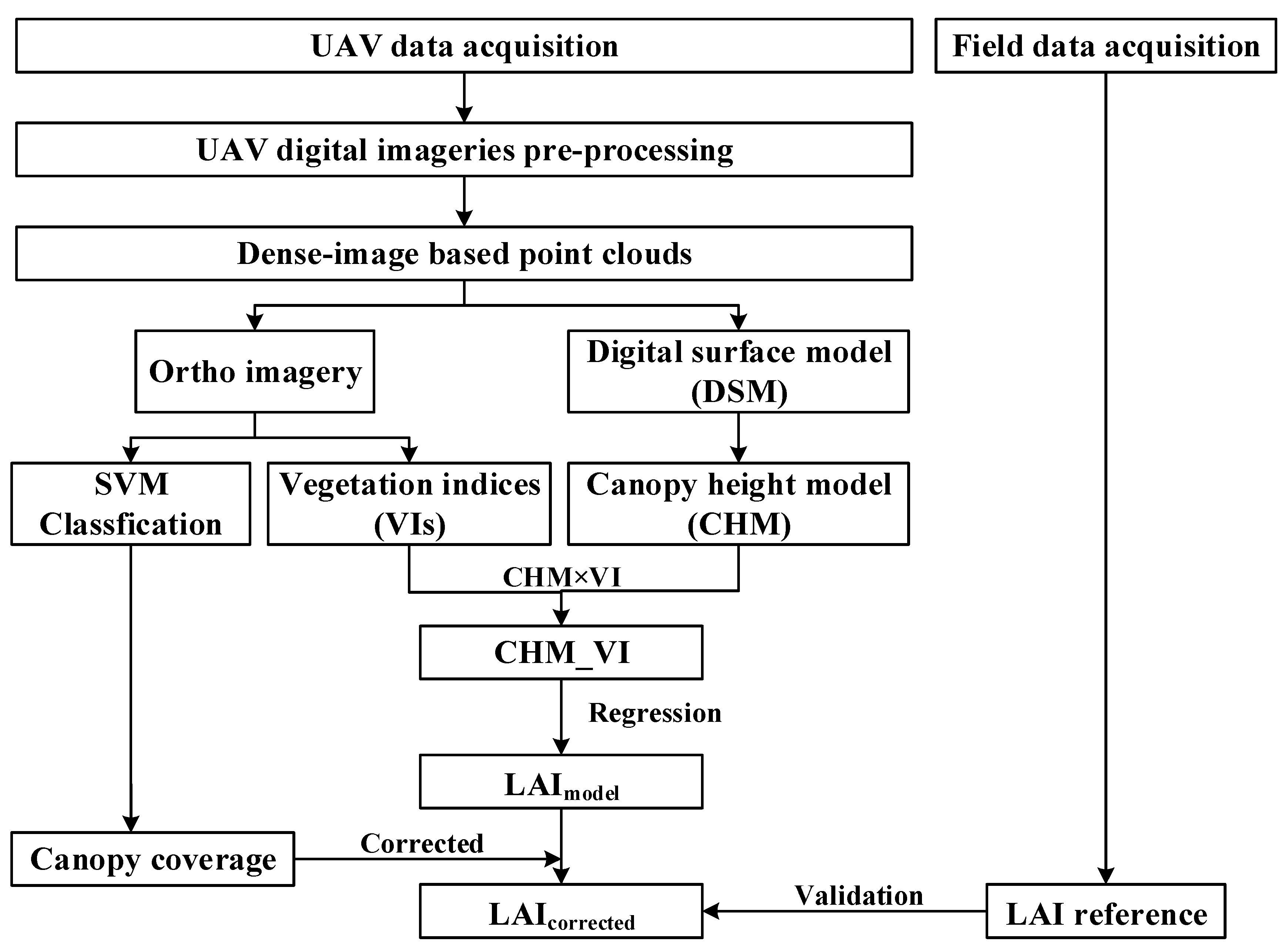
LAI was obtained using the LAI-2200C vegetation canopy analyzer before 10:00 a.m. on the same day as the UAV flights. To minimize measurement errors, thirteen independent measurements were taken for each quadrat, and the average of thirteen readings was calculated as the ground truth of LAI in each quadrat. In this study, 80 quadrats with different degrees of density were measured, all of which were used for subsequent analysis. In order to verify the accuracy of the canopy height model, the experiment measured the wheat canopy height with a ruler, and the minimum measurement unit was 1 mm. In the experiment, 10 wheat plants were randomly selected in each quadrat to measure their plant height, and the average value was calculated as the measured canopy height of the quadrat. The geographic coordinates of the quadrats were recorded using GNSS RTK device to match the UAV images with the corresponding quadrats.

2.4. Method

2.4.1. An Improved LAI Estimation Method

An improved LAI estimation method proposed in this study mainly includes three steps: (1) Extract wheat canopy spectral information (vegetation index (VI)) and wheat growth characteristics (canopy height (CHM) and canopy coverage (CC)) based on UAV images; (2) The vegetation index weighted canopy height model obtains the remote sensing index CHM_VI; (3) The LAI estimation model based on CHM_VI was corrected by using CC as a correction parameter. The overall flow of this method to estimate LAI is shown in Figure 3.

The essence of an improved LAI estimation method is to further improve the LAI estimation accuracy by incorporating the crop canopy height and coverage on the basis of spectral information. Among them, canopy height and vegetation index were used to construct the LAI estimation model, and CC was used as a correction parameter to optimize the performance of the estimation model. The study estimated the final wheat LAI by Equations (1) and (2).

LAI_corrected = LAI_model × CC

(1)

LAI_model = F (CHM, VI)

(2)

where LAI_corrected is the final LAI estimate after CC correction, LAI_model is the original LAI estimate based on the empirical model, and F is the linear regression function, CHM and VI are the characteristic variables for estimating LAI. The research used CHM to adjust VI in a weighted manner to generate CHM_VI, and then establishes an empirical model of CHM_VI and LAI for LAI estimation. Its calculation formula is as follows:

CHM_VI = CHM × VI_Rmax

(3)

In the Equation (3), VI_Rmax is a vegetation index with the highest correlation with LAI. The VI_Rmax and CHM were combined in the form of multiplication (VI_Rmax ∗ CHM) to establish LAI regression models [26].

For the calculation of sample values of CHM and VI, a square buffer with a side length of 2 m was first generated for each quadrat, and then the VI and CHM values of all pixels in the region were averaged to express the VI value and CHM value of the quadrats.

2.4.2. Vegetation Index (VI) Calculation

In order to evaluate the correlation between different VIs and LAI, and to find the most correlated multispectral vegetation indices (MS-VIs) and visible light vegetation indices (RGB-VIs) among VIs for LAI estimation, a series of published optical indices, including five MS-VIs and five RGB-VIs, were calculated by the formulas shown in

Table 2. Definition of the selected VIs.

Vegetation Index	Formula 1	Reference
Excess Green Index (ExG)	2 g – r − b	[34]
Excess Green minus Excess Red Index (ExGR)	3 g − 2.4 r − b	[33]
Normalized Green minus Red Difference Index (NGRDI)	(g − r)/(g + r)	[34]
Visible Atmospherically Resistant Index (VARI)	(g − r)/(g + r − b)	[35]
Green Leaf Index (GLI)	(2 g – b − r)/(2 g + b + r)	[36]
Red-edge Normalized Difference Vegetation Index (NDRE)	(pnir − pred edge)/(pnir + pred edge)	[37]
Normalized Difference Vegetation Index (NDVI)	(pnir − pred)/(pnir + pred)	[38]
Green Normalized Difference Vegetation Index (GNDVI)	(pnir − pgreen)/(pnir + pgreen)	[39]
Difference Vegetation Index (DVI)	pnir − pred	[40]
Optimized Soil Adjusted Vegetation Index (OSAVI)	(1 + 0.16) × (pnir − pred)/(pnir + pred + 0.16)	[41]

¹ Wavelengths of p_red, p_green, p_bule, p_{red edge}, and p_nir were 475, 560, 668, 717, and 842 nm. g = G/(R + G + B), r = R/(R + G + B), b = B/(R + G + B). R, G, and B represent the mean digital number values of each quadrat derived from RGB images, which range from 0 to 255.

. These indices have all been proven to be useful indicators of vegetation growth and were commonly used in crop growth monitoring and vegetation detection. MS-VIs were calculated from multispectral images using the mean value (i.e., spectral reflectance) of each quadrat, while RGB-VIs were calculated using re-normalized r, g, and b bands [33].

The correlations between the above ten VIs and LAI are shown in

Table 3. Correlation coefficient (R) between image-derived information and LAI.

Index Type	Spectral Index	Pearson Correlation Coefficient (R)
RGB-VIs	ExG	0.433 **
	ExGR	0.408 **
	NGRDI	0.379 **
	VARI	0.372 **
	GLI	0.434 **
MS-VIs	NDRE	0.729 **
	NDVI	0.570 **
	GNDVI	0.727 **
	DVI	0.453 **
	OSAVI	0.542 **

The highest r value for each type of metrics is highlighted in boldface. Description for each index and metric referred to Table 2. ** Correlation is significant at the 0.01 level (2-tailed).

.

The results showed that all vegetation indices selected in the experiment were significantly correlated with LAI. Among them, the indices with relatively highest correlation coefficient values in MS-VIs and RGB-VIs were NDRE (R = 0.729) and GLI (R = 0.434), respectively. Therefore, in this study, the best spectral features for estimating wheat LAI from RGB imagery and multispectral imagery were GLI and NDRE, respectively, and the LAI estimation model is constructed on this basis.

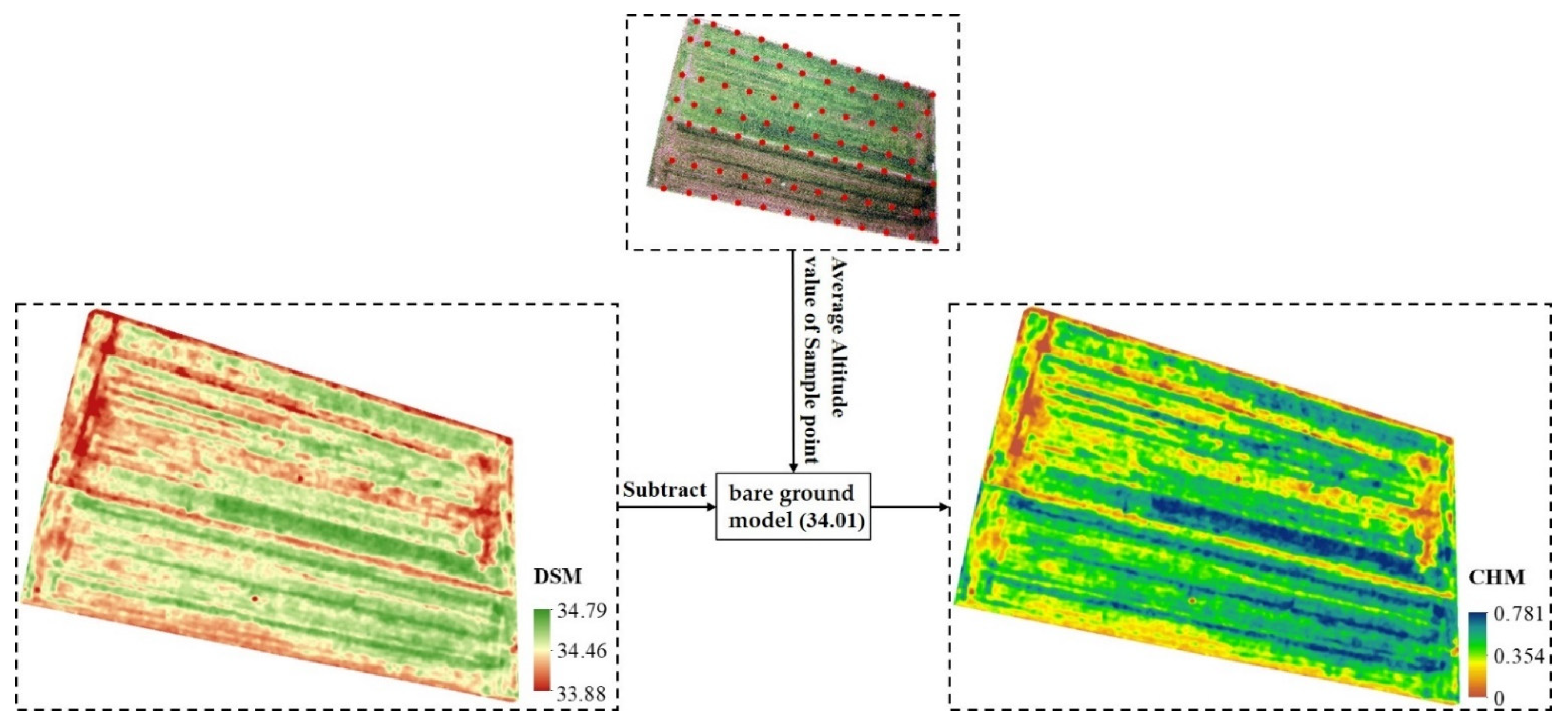
2.4.3. Canopy Height and Coverage Extraction

The Canopy Height Model (CHM) represents the height of vegetation growth. To get the CHM, the digital surface model (DSM) generated by the photogrammetric point clouds was subtracted from the bare ground DSM [28] (Figure 4). The bare ground model was represented by a constant that was the mean of all quadrat elevations measured with GNSS RTK. Because the terrain of the study area is flat, the quadrat was evenly distributed throughout the study area, and the standard deviation of the elevation of the quadrat is only 0.056 m, so it is feasible to use the average elevation of the quadrat in the study area as the bare ground model of the flat wheat field. The above operations were performed in ArcGIS10.5 software.

In the experiment, the canopy coverage of all quadrats was calculated according to Equation (4).

$$\mathrm{CC}=\frac{{\mathrm{A}}_{\mathrm{vegetation}}}{{\mathrm{A}}_{\mathrm{all}}}$$

(4)

In the formula, ${\mathrm{A}}_{\mathrm{vegetation}}$ represents the area of vegetation in the quadrat, and ${\mathrm{A}}_{\mathrm{all}}$ represents the area of the entire quadrat.

The study used support vector machine (SVM) to classify the entire study area, dividing the objects in the study area into two categories: vegetation and non-vegetation, and then counting the area occupied by vegetation in the quadrat to calculate CC of each quadrat. The entire quadrat dataset was divided into sparse canopy structure dataset and closed canopy structure dataset based on CC to explore the difference in estimation performance under different canopy structures. The quadrats with CC less than 90% were classified as sparse dataset, and the remaining ones were classified as closed dataset.

2.5. Evaluation Method

Based on the entire dataset (80 quadrats), closed dataset (39 quadrats), and sparse dataset (41 quadrats), the LAI estimation results obtained by the traditional method and the improved LAI estimation method were compared with on-site measurement for accuracy evaluation. The performance of the LAI estimation model was assessed using the Coefficient of determination (R²), Root mean square error (RMSE) and Normalized Root mean square error (NRMSE), and its expression is shown in Equations (5)–(7). Origin 2017 software was used for modeling and the production of result graphs.

$${\mathrm{R}}^2=\frac{{{\displaystyle \sum }}_1^{\mathrm{n}}{\left({\mathrm{x}}_{\mathrm{i}}-\overline{\mathrm{x}}\right)}^2{\left({\mathrm{y}}_{\mathrm{i}}-\overline{\mathrm{y}}\right)}^2}{\mathrm{n}{{\displaystyle \sum }}_1^{\mathrm{n}}{\left({\mathrm{x}}_{\mathrm{i}}-\overline{\mathrm{x}}\right)}^2{{\displaystyle \sum }}_1^{\mathrm{n}}{\left({\mathrm{y}}_{\mathrm{i}}-\overline{\mathrm{y}}\right)}^2}$$

(5)

$$\mathrm{RMSE}=\sqrt{\frac{{{\displaystyle \sum }}_1^{\mathrm{n}}{\left({\mathrm{p}}_{\mathrm{i}}-{\mathrm{q}}_{\mathrm{i}}\right)}^2}{\mathrm{n}}}$$

(6)

$$\mathrm{NRMSE} =\frac{\mathrm{RMSE}}{\overline{\mathrm{q}}}$$

(7)

In the formula: n is the number of samples; ${\mathrm{x}}_{\mathrm{i}}$, ${\mathrm{y}}_{\mathrm{i}}$, $\overline{\mathrm{x}},$ and $\overline{\mathrm{y}},$ represent the independent variable value, dependent variable value, independent variable mean value, and dependent variable mean value involved in the model, respectively; ${\mathrm{p}}_{\mathrm{i}}$ is the estimated value of the model; ${\mathrm{q}}_{\mathrm{i}}$ is the field observed value, $\overline{\mathrm{q}}$ is the mean value of field observations.

3. Results

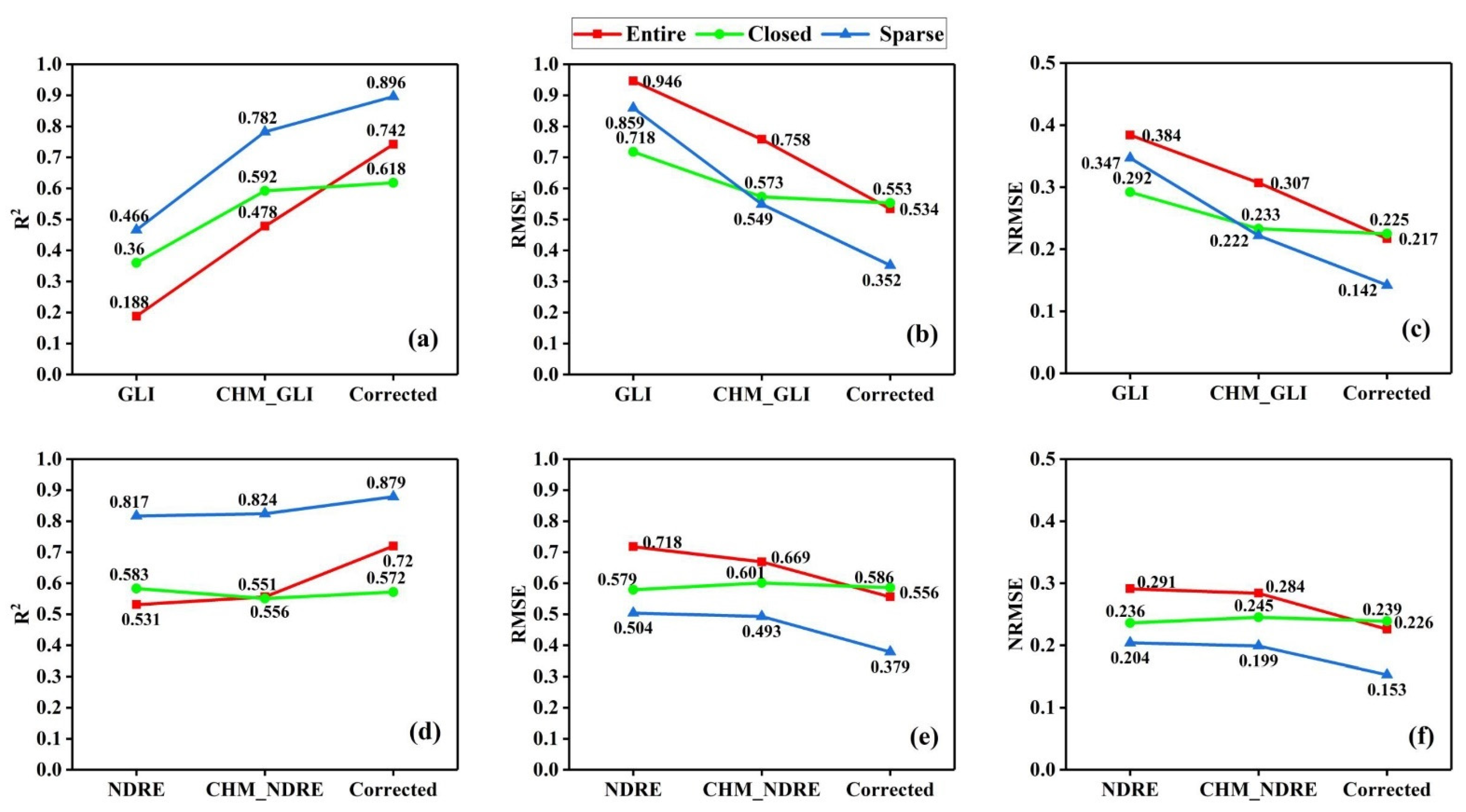
3.1. LAI Estimation Accuracy

Based on the vegetation index GLI and NDRE calculated from UAV RGB and multispectral images, the research compared the accuracy of LAI estimation by the traditional method only using vegetation index and the improved method proposed in this experiment (incorporating with CHM and CC). The results are shown in Figure 5.

From the entire dataset, the R² of the LAI estimated by the GLI and the improved method was 0.188 and 0.742, the RMSE was 0.946 and 0.534, the NRMSE was 0.384 and 0.217, respectively, and the RMSE decreased by 43.6%. The R² of the LAI estimated by the NDRE and the improved method was 0.531 and 0.72, the RMSE was 0.718 and 0.556, the NRMSE was 0.291 and 0.226, respectively, and the RMSE decreased by 22.6%. The results show that the improved LAI estimation method combined with CHM and CC correction on the basis of the original vegetation index can significantly improve the LAI estimation accuracy. Both RGB images and multispectral images showed good results, but the improvement of RGB images is more prominent. The improved method performs similarly on closed and sparse datasets.

3.2. Influence of Canopy Height

In order to explore the influence of canopy height on LAI estimation, for RGB images, two empirical models were constructed to estimate LAI using GLI and CHM_GLI obtained from GLI weighted CHM, respectively. For multispectral images, two other empirical models were constructed to estimate LAI using NDRE and CHM_NDRE obtained from NDRE weighted CHM, respectively. The performance of the four models on different canopy structure datasets was shown in Figure 6.

It can be seen from Figure 6 that the RGB-VI (GLI) calculated based on the RGB imagery, combined with CHM, performs well in the LAI estimation of different datasets. In the entire dataset (Figure 6d: R² = 0.478, RMSE = 0.758, NRMSE = 0.307), closed dataset (Figure 6e: R² = 0.592, RMSE = 0.573, NRMSE = 0.233) and sparse dataset (Figure 6f: R² = 0.782, RMSE = 0.549, NRMSE = 0.222), compared with the GLI estimation model, the CHM_GLI estimation model significantly improves R², while the RMSE and NRMSE decrease. It shows that RGB-VIs can significantly improve the LAI estimation accuracy when combined with CHM. Therefore, when we conduct the estimation of crop LAI, canopy height can also be used as one of the effective features, and its addition can improve the estimation performance of LAI to a certain extent. Especially when the acquired spectral information is limited (RGB imagery), canopy height can be used as an effective information to make up for the lack of spectral information, thereby improving the estimation accuracy of crop LAI.

The MS-VI (NDRE) calculated based on the multispectral imagery, combined with CHM, performed well in the LAI estimation of different datasets. However, in the entire dataset (Figure 6j: R² = 0.556, RMSE = 0.669, NRMSE = 0.284), closed dataset (Figure 6k: R² = 0.551, RMSE = 0.601, NRMSE = 0.245), and sparse dataset (Figure 6l: R² = 0.824, RMSE = 0.493, NRMSE = 0.199), compared with the NDRE estimation model, the CHM_NDRE estimation model has no significant improvement in the LAI estimation accuracy. It can be seen that the canopy height information was more conducive to improving the accuracy of LAI estimation in RGB images with weak spectral information. For multispectral images with strong spectral information, better LAI estimation performance can be obtained only based on the spectral information (Figure 6g–i), and the addition of CHM had no significant effect on it.

The experiments also found that when the measured LAI value was small or the canopy structure was sparse, the model overestimated the LAI. Therefore, the canopy structure of wheat appears to affect the performance of the model for LAI estimation. To account for the impact of canopy structure on LAI estimation, the performance of the LAI estimation model was tested with entire, closed, and sparse datasets. The LAI estimation performance based on the GLI model is quite different among the three datasets (Figure 6a–c). In contrast, the closed dataset (Figure 6a: R² = 0.36, RMSE = 0.718, NRMSE = 0.292) had better estimation performance than the entire dataset (Figure 6b: R² = 0.188, RMSE = 0.946, NRMSE = 0.384). Although the R² of the sparse dataset (Figure 6c: R² = 0.466, RMSE = 0.859, NRMSE = 0.347) is slightly higher, both RMSE and NRMSE were larger than those of the closed dataset, and there was an overall LAI overestimation. In addition to this, the LAI estimation performance of other models also had obvious differences between different datasets. Thus, the canopy structure of wheat is a critical element affecting the performance of the model on LAI estimation.

3.3. Influence of CC Correction

As mentioned in Section 3.2, there was an overestimation in the model estimation at low LAI values. Therefore, we tried to use CC to correct the estimation results and explore whether CC would affect LAI estimation positively. Figure 7 shows that R² increased and both RMSE and NRMSE decreased after the correction for all datasets, indicating that CC has a positive impact on LAI estimation performance. However, the effects of CC on the estimation results varied with the datasets. The correction effects on the LAI estimation model were significant on the entire dataset and sparse dataset, while it was not large on the closed dataset.

Based on RGB imagery (Figure 7a–c), after CC correction, NRMSE decreased by 29.32% on the entire dataset and by 36.04% on the sparse dataset, but only by 3.43% on the closed dataset. The CC in the closed dataset was above 90% in every quadrat, so the correction would not have much impact. In general, CC correction can greatly improve the accuracy of LAI estimation from RGB images, except in areas where wheat is very densely grown. Based on multispectral imagery (Figure 7d–f), after CC correction, NRMSE decreased by 20.42% on the entire dataset and by 23.12% on the sparse dataset, but only by 2.45% on the closed dataset. This had a similar performance to RGB imagery. For multispectral imagery, CC correction can also improve the estimation accuracy of LAI, but the improvement effect was not as good as that of RGB imagery.

4. Discussion

4.1. The Role of UAV Remote Sensing

Canopy structure information is a key factor to improve the LAI estimation accuracy in this study. For field crops, neither ground-based measuring instruments nor satellite remote sensing can accurately obtain crop structure information. However, with the advantages of ultra-high resolution and photogrammetry technology, UAV remote sensing can not only obtain crop canopy point clouds but also accurately calculate canopy coverage. Therefore, UAV remote sensing plays an important role in precision agriculture.

In this study, crop canopy height and coverage were defined as crop growth characteristics. As a structural parameter, LAI is closely related to crop growth. Theoretically, the taller the crop is, the more leaves it will produce, which means that within a unit area, a taller crop will produce a larger unit leaf area, and the corresponding LAI will be larger. Therefore, crop height and LAI are correlated. Taking crop canopy height as one of the characteristics of LAI estimation will effectively improve the accuracy of LAI estimation, and previous studies have also reached similar conclusions [42,43,44]. In our method, the canopy height and the vegetation index were combined in a multiplicative manner, and the effectiveness of this manner has been proved in previous studies on monitoring the growth of rapeseed [26], which can effectively avoid the problem of weight selection. Ensuring the accuracy of crop height information extraction is a key step before applying height information to the features of crop LAI estimation. In this study, the canopy height model (CHM) of crops was extracted by UAV photogrammetry. To be precise, it is obtained by subtracting the bare ground DSM from the DSM generated by UAV photogrammetry. Among them, the bare ground DSM is replaced by the average elevation of all sample quadrats, and there were two main reasons why this was possible. First, the terrain of the study area is flat, the quadrats are evenly distributed in the whole study area, and the standard deviation of elevation of all quadrats is only 0.056 m. Second, it is difficult to obtain enough ground points in the densely growing wheat field for the point cloud of UAV photogrammetry. When the number of ground points is insufficient, the accuracy of the constructed bare-ground DSM cannot meet the requirements. Therefore, according to the actual situation of the study area, the crop canopy height extraction method proposed in this study is relatively more accurate. If the wheat field has a certain slope, we need to separate the ground points from the photogrammetric point cloud to construct the bare ground DSM to estimate the canopy height. This does not affect the LAI estimation method proposed in this paper needing to select the appropriate bare ground DSM according to the field situation.

In research experiments, the correlation and deviation between the canopy height obtained by UAV photogrammetry and the canopy height measured in situ were calculated (R² = 0.778, RMSE = 0.027). Although the fitting accuracy of the canopy height was high, there was also a certain error. This part of the reason was due to the fact that the sample was a plot scale (2 m × 2 m quadrat), as the study cannot use GPS to accurately locate each wheat plant, so there was a certain error in using the average height of 10 wheat plants as the wheat canopy height of the entire quadrat. Another part of the reason was the error of the DSM itself obtained by photogrammetry. Overall, the estimated canopy height in this study exhibits strong agreement with ground measurements based on error metrics (RMSE = 0.027 m). Similar results were also observed in other studies [45,46].

The leaf area index (LAI) is defined as the ratio of one-sided leaf area per unit of ground area [47]. By definition, higher coverage means a higher ratio of leaf area per unit ground area. Some studies have found that canopy coverage has a good correlation with LAI [48,49,50], which is also the premise that this study can use canopy coverage as a correction parameter to improve the accuracy of LAI estimation. Due to the structural characteristics of wheat leaves, it is almost impossible for the canopy of wheat crops to close. Therefore, when studying the biophysical parameters of wheat at the plot scale, the canopy spectral values obtained from UAV images will be affected by the soil background to a certain extent. In the process of wheat LAI estimation, the ground-measured LAI corresponds to the heterogeneous canopy spectral index, which eventually leads to a certain degree of LAI overestimation. To solve the above problem, CC was introduced as a correction parameter to optimize estimated LAI values. Removing the soil background could bring the crop canopy closer to the ideal state, and CC can offset the influence of removing the soil background on the average reflectance. Thus, CC played an important role in improving the estimation performance.

4.2. Potential of RGB Images

An improved LAI estimation method, incorporating growth characteristics of field-grown wheat introduced in this study, shows different effects on RGB images and multispectral images. Compared with multispectral images, this method improves the accuracy of LAI estimation based on RGB images more obviously. In fact, the multispectral imagery contains more abundant spectral information, and the wheat LAI can be well estimated only by the multispectral information, so it is difficult to greatly improve the estimation accuracy with the addition of structural information. However, the spectral information of the RGB imagery itself is weak, and it is difficult to effectively monitor the wheat LAI only from the visible light band. At this time, it is particularly important for LAI estimation to add the structural parameters related to the LAI. In agricultural applications, visible light sensors have low cost and high resolution. Many scholars have conducted corresponding research on monitoring crop growth and inversion of relevant biophysical parameters from RGB images. For example, Zhang et al. [51] applied airborne RGB images to effectively classify crops and estimate leaf area index for a 6.5 km² crop planting area. Yan et al. [17] improved the estimation of fractional vegetation cover from UAV RGB imagery by color unmixing. Maitiniyazi et al. introduced an efficient approach for using low-cost, high-resolution UAS RGB imagery to accurately estimate soybean AGB. Those all indicate that RGB images have great potential in precision agriculture or agricultural production monitoring. The improved LAI estimation method proposed in this study also performs well on RGB images. As can be seen from Figure 5, after the RGB-VI GLI was combined with the growth characteristics, its LAI estimation effect can already reach a performance similar to that of multispectral images. In addition, the use of digital cameras instead of multispectral cameras for agricultural research reduces the requirements for light conditions during UAV data collection to a certain extent, makes UAV data acquisition more flexible, and enriches agricultural managers’ crop monitoring methods.

4.3. Estimation Method

There are two main approaches to estimate LAI or other biophysical parameters using remote sensing data: radiative transfer models (RTMs) and empirical statistical models (ESMs). Typical empirical algorithms for LAI estimation are mostly based on a simple vegetation index (VI) or spectral transform values to build an estimation model [52,53,54,55]. This study combined VI with the structural features of high-resolution remote sensing images into a new VI to construct a more accurate ESM, and the results demonstrate that this method could improve the accuracy of wheat LAI estimation. Although ESM methods are simple, efficient, and widely applicable, they may not be generally applicable to other settings due to their reliance on specific modeling datasets for empirical relationships. Therefore, in order to achieve a more comprehensive and accurate LAI estimation, it is necessary to explore more LAI remote sensing acquisition methods.

UAV remote sensing can obtain high-resolution remote sensing images of various altitudes and angles by virtue of its advantages. However, the current LAI estimation using UAV remote sensing data still uses the above-mentioned traditional methods and does not fully utilize the advantages of UAV remote sensing. In the future, referring to the principle of the Plant Canopy Analyzer (LAI-2200), based on Beer’s Law, a new LAI measurement method can be explored by using the multi-angle data of UAV. This will not only get rid of the uncertainty of traditional inversion methods, but also provide a new type of planar LAI measurement data.

5. Conclusions

This study proposed an improved LAI estimation method, combining spectral characteristics and crop growth characteristics (canopy height and coverage) to improve the accuracy of wheat LAI estimation based on UAV images. The main conclusions are as follows: (1) The proposed method can improve the LAI estimation accuracy on both UAV RGB imagery and multispectral imagery, especially on RGB imagery; (2) Canopy height is correlated with LAI, and the introduction of CHM will significantly improve the LAI estimation accuracy; (3) CC correction can improve the performance of LAI estimation under non-closed canopy structure. This study provides a robust, practical, and low-cost method for accurately estimate wheat leaf area index using UAV remote sensing data. The research enriches the ways of using digital cameras for crop growth monitoring, which can provide a reference for reducing the cost of agricultural production monitoring. Future research should be extended to rice, soybean, maize, and other crops to develop a general and crop-independent LAI estimation method.

References

1. Gower, S.T.; Kucharik, C.J.; Norman, J.M. Direct and Indirect Estimation of Leaf Area Index, f APAR, and Net Primary Production of Terrestrial Ecosystems. Remote Sens. Environ. 1999, 70, 29–51. [Google Scholar] [CrossRef]
2. Brisco, B.; Brown, R.J.; Hirose, T.; McNairn, H.; Staenz, K. Precision Agriculture and the Role of Remote Sensing: A Review. Can. J. Remote Sens. 1998, 24, 315–327. [Google Scholar] [CrossRef]
3. Marshall, M.; Thenkabail, P. Developing in situ Non-Destructive Estimates of Crop Biomass to Address Issues of Scale in Remote Sensing. Remote Sens. 2015, 7, 808–835. [Google Scholar] [CrossRef]
4. Zhou, X.; Zheng, H.B.; Xu, X.Q.; He, J.Y.; Ge, X.K.; Yao, X.; Cheng, T.; Zhu, Y.; Cao, W.X.; Tian, Y.C. Predicting grain yield in rice using multi-temporal vegetation indices from UAV-based multispectral and digital imagery. ISPRS J. Photogramm. 2017, 130, 246–255. [Google Scholar] [CrossRef]
5. Thenkabail, P.S.; Gumma, M.K.; Teluguntla, P.; Mohammed, I.A. Hyperspectral remote sensing of vegetation and agricultural crops. Photogramm. Eng. Remote Sens. J. Am. Soc. Photogramm. 2014, 80, 695–723. [Google Scholar]
6. Broge, N.H.; Leblanc, E. Comparing prediction power and stability of broadband and hyperspectral vegetation indices for estimation of green leaf area index and canopy chlorophyll density. Remote Sens. Environ. 2001, 76, 156–172. [Google Scholar] [CrossRef]
7. Viña, A.; Gitelson, A.A.; Nguy-Robertson, A.L.; Peng, Y. Comparison of different vegetation indices for the remote assessment of green leaf area index of crops. Remote Sens. Environ. 2011, 115, 3468–3478. [Google Scholar] [CrossRef]
8. Sha, Z.; Wang, Y.; Bai, Y.; Zhao, Y.; Jin, H.; Na, Y.; Meng, X. Comparison of leaf area index inversion for grassland vegetation through remotely sensed spectra by unmanned aerial vehicle and field-based spectroradiometer. J. Plant Ecol. 2018, 12, 395–408. [Google Scholar] [CrossRef]
9. Feret, J.; François, C.; Asner, G.P.; Gitelson, A.A.; Martin, R.E.; Bidel, L.P.R.; Ustin, S.L.; le Maire, G.; Jacquemoud, S. PROSPECT-4 and 5: Advances in the leaf optical properties model separating photosynthetic pigments. Remote Sens. Environ. 2008, 112, 3030–3043. [Google Scholar] [CrossRef]
10. Lang, Q.; Weijie, T.; Dehua, G.; Ruomei, Z.; Lulu, A.; Minzan, L.; Hong, S.; Di, S. UAV-based chlorophyll content estimation by evaluating vegetation index responses under different crop coverages. Comput. Electron. Agric. 2022, 196, 106775. [Google Scholar]
11. Amarasingam, N.; Felipe, G.; Ashan, S.A.S.; Madhushanka, K.U.W.L.; Sampageeth, W.H.A.; Rasanjana, K.B. Predicting Canopy Chlorophyll Content in Sugarcane Crops Using Machine Learning Algorithms and Spectral Vegetation Indices Derived from UAV Multispectral Imagery. Remote Sens. 2022, 14, 11140. [Google Scholar]
12. Thenkabail, P.S.; Smith, R.B.; De Pauw, E. Hyperspectral Vegetation Indices and Their Relationships with Agricultural Crop Characteristics. Remote Sens. Environ. 2000, 71, 158–182. [Google Scholar] [CrossRef]
13. Hansen, P.M.; Schjoerring, J.K. Reflectance measurement of canopy biomass and nitrogen status in wheat crops using normalized difference vegetation indices and partial least squares regression. Remote Sens. Environ. 2003, 86, 542–553. [Google Scholar] [CrossRef]
14. Dezhi, W.; Bo, W.; Jing, L.; Yanjun, S.; Qinghua, G.; Penghua, Q.; Xincai, W. Estimating aboveground biomass of the mangrove forests on northeast Hainan Island in China using an upscaling method from field plots, UAV-LiDAR data and Sentinel-2 imagery. Int. J. Appl. Earth Obs. 2020, 85, 101986. [Google Scholar]
15. Zhang, J.; Qiu, X.; Wu, Y.; Zhu, Y.; Cao, Q.; Liu, X.; Cao, W. Combining texture, color, and vegetation indices from fixed-wing UAS imagery to estimate wheat growth parameters using multivariate regression methods. Comput. Electron. Agric. 2021, 185, 106138. [Google Scholar] [CrossRef]
16. Maimaitijiang, M.; Sagan, V.; Sidike, P.; Maimaitiyiming, M.; Hartling, S.; Peterson, K.T.; Maw, M.J.W.; Shakoor, N.; Mockler, T.; Fritschi, F.B. Vegetation Index Weighted Canopy Volume Model (CVMVI) for soybean biomass estimation from Unmanned Aerial System-based RGB imagery. ISPRS J. Photogramm. 2019, 151, 27–41. [Google Scholar] [CrossRef]
17. Yan, G.; Li, L.; Coy, A.; Mu, X.; Chen, S.; Xie, D.; Zhang, W.; Shen, Q.; Zhou, H. Improving the estimation of fractional vegetation cover from UAV RGB imagery by colour unmixing. ISPRS J. Photogramm. 2019, 158, 23–34. [Google Scholar] [CrossRef]
18. Zhang, J.; Liu, X.; Liang, Y.; Cao, Q.; Tian, Y.; Zhu, Y.; Cao, W.; Liu, X. Using a Portable Active Sensor to Monitor Growth Parameters and Predict Grain Yield of Winter Wheat. Sensors 2019, 19, 1108. [Google Scholar] [CrossRef]
19. Hassan, M.A.; Yang, M.; Rasheed, A.; Yang, G.; Reynolds, M.; Xia, X.; Xiao, Y.; He, Z. A rapid monitoring of NDVI across the wheat growth cycle for grain yield prediction using a multi-spectral UAV platform. Plant Sci. 2019, 282, 95–103. [Google Scholar] [CrossRef]
20. Martin, K.; Insa, K.; Dieter, T.; Thomas, J. High-Resolution UAV-Based Hyperspectral Imagery for LAI and Chlorophyll Estimations from Wheat for Yield Prediction. Remote Sens. 2018, 10, 2000. [Google Scholar]
21. Songyang, L.; Xingzhong, D.; Qianliang, K.; Tahir, A.S.; Tao, C.; Xiaojun, L.; Yongchao, T.; Yan, Z.; Weixing, C.; Qiang, C. Potential of UAV-Based Active Sensing for Monitoring Rice Leaf Nitrogen Status. Front. Plant Sci. 2018, 9, 1834. [Google Scholar]
22. Yao, X.; Wang, N.; Liu, Y.; Cheng, T.; Tian, Y.; Chen, Q.; Zhu, Y. Estimation of Wheat LAI at Middle to High Levels Using Unmanned Aerial Vehicle Narrowband Multispectral Imagery. Remote Sens. 2017, 9, 1304. [Google Scholar] [CrossRef]
23. Zhu, W.; Sun, Z.; Huang, Y.; Lai, J.; Li, J.; Zhang, J.; Yang, B.; Li, B.; Li, S.; Zhu, K.; et al. Improving Field-Scale Wheat LAI Retrieval Based on UAV Remote-Sensing Observations and Optimized VI-LUTs. Remote Sens. 2019, 11, 2456. [Google Scholar] [CrossRef]
24. Dandois, J.P.; Ellis, E.C. High spatial resolution three-dimensional mapping of vegetation spectral dynamics using computer vision. Remote Sens. Environ. 2013, 136, 259–276. [Google Scholar] [CrossRef]
25. Puliti, S.; Ørka, H.; Gobakken, T.; Næsset, E. Inventory of Small Forest Areas Using an Unmanned Aerial System. Remote Sens. 2015, 7, 9632–9654. [Google Scholar] [CrossRef]
26. Zhang, J.; Wang, C.; Yang, C.; Xie, T.; Jiang, Z.; Hu, T.; Luo, Z.; Zhou, G.; Xie, J. Assessing the Effect of Real Spatial Resolution of In Situ UAV Multispectral Images on Seedling Rapeseed Growth Monitoring. Remote Sens. 2020, 12, 1207. [Google Scholar] [CrossRef]
27. Cunliffe, A.M.; Brazier, R.E.; Anderson, K. Ultra-fine grain landscape-scale quantification of dryland vegetation structure with drone-acquired structure-from-motion photogrammetry. Remote Sens. Environ. 2016, 183, 129–143. [Google Scholar] [CrossRef]
28. Bendig, J.; Yu, K.; Aasen, H.; Bolten, A.; Bennertz, S.; Broscheit, J.; Gnyp, M.L.; Bareth, G. Combining UAV-based plant height from crop surface models, visible, and near infrared vegetation indices for biomass monitoring in barley. Int. J. Appl. Earth Obs. Geoinf. 2015, 39, 79–87. [Google Scholar] [CrossRef]
29. Giannetti, F.; Chirici, G.; Gobakken, T.; Næsset, E.; Travaglini, D.; Puliti, S. A new approach with DTM-independent metrics for forest growing stock prediction using UAV photogrammetric data. Remote Sens. Environ. 2018, 213, 195–205. [Google Scholar] [CrossRef]
30. Heidarian Dehkordi, R.; Burgeon, V.; Fouche, J.; Placencia Gomez, E.; Cornelis, J.; Nguyen, F.; Denis, A.; Meersmans, J. Using UAV Collected RGB and Multispectral Images to Evaluate Winter Wheat Performance across a Site Characterized by Century-Old Biochar Patches in Belgium. Remote Sens. 2020, 12, 2504. [Google Scholar] [CrossRef]
31. Zhang, D.; Liu, J.; Ni, W.; Sun, G.; Zhang, Z.; Liu, Q.; Wang, Q. Estimation of Forest Leaf Area Index Using Height and Canopy Cover Information Extracted From Unmanned Aerial Vehicle Stereo Imagery. IEEE J. Stars 2019, 12, 471–481. [Google Scholar] [CrossRef]
32. Sun, B.; Wang, C.; Yang, C.; Xu, B.; Zhou, G.; Li, X.; Xie, J.; Xu, S.; Liu, B.; Xie, T.; et al. Retrieval of rapeseed leaf area index using the PROSAIL model with canopy coverage derived from UAV images as a correction parameter. Int. J. Appl. Earth Obs. 2021, 102, 102373. [Google Scholar] [CrossRef]
33. Meyer, G.E.; Neto, J.C. Verification of color vegetation indices for automated crop imaging applications. Comput. Electron. Agric. 2008, 63, 282–293. [Google Scholar] [CrossRef]
34. Woebbecke, D.M.U.O.; Meyer, G.E.; Von Bargen, K.; Mortensen, D.A. Color Indices for Weed Identification Under Various Soil, Residue, and Lighting Conditions. Trans. ASAE 1995, 38, 259–269. [Google Scholar] [CrossRef]
35. Gitelson, A.A.; Kaufman, Y.J.; Stark, R.; Rundquist, D. Novel algorithms for remote estimation of vegetation fraction. Remote Sens. Environ. 2002, 80, 76–87. [Google Scholar] [CrossRef]
36. Mounir, L.; Michael, M.B.; Douglas, E.J. Spatially Located Platform and Aerial Photography for Documentation of Grazing Impacts on Wheat. Geocarto Int. 2001, 16, 65–70. [Google Scholar]
37. Anatoly, G.; Merzlyak, M.N. Spectral Reflectance Changes Associated with Autumn Senescence of Aesculus hippocastanum L. and Acer platanoides L. Leaves. Spectral Features and Relation to Chlorophyll Estimation. Urban Fischer 1994, 143, 286–292. [Google Scholar]
38. Peñuelas, J.; Isla, R.; Filella, I.; Araus, J.L. Visible and Near-Infrared Reflectance Assessment of Salinity Effects on Barley. Crop Sci. 1997, 37, 198–202. [Google Scholar] [CrossRef]
39. Gitelson, A.A.; Kaufman, Y.J.; Merzlyak, M.N. Use of a green channel in remote sensing of global vegetation from EOS-MODIS. Remote Sens. Environ. 1996, 58, 289–298. [Google Scholar] [CrossRef]
40. Jordan, C.F. Derivation of Leaf-Area Index from Quality of Light on the Forest Floor. Ecology 1969, 50, 663–666. [Google Scholar] [CrossRef]
41. Rondeaux, G.; Steven, M.; Baret, F. Optimization of soil-adjusted vegetation indices. Remote Sens. Environ. 1996, 55, 95–107. [Google Scholar] [CrossRef]
42. Ortega, G.A.; Henrique, F.M.D.S.; Goncalves, G.L.; Mantelatto, R.J.; Stephanie, C.; Martins, F.J.I.; Ricardo, M.F. Improving indirect measurements of the lea area index using canopy height. Pesqui. Agropecu. Bras. 2020, 55. [Google Scholar] [CrossRef]
43. Jose, C.J.; Rodrigo, D.S.S.E.; Vieira, D.C.M.; Virginia, F.D.S.M.; Carlos, B.D.J.J.; de Mello Alexandre Carneiro, L. Correlations between plant height and light interception in grasses by different light meter devices. Rev. Bras. De Cienc. Agrar. Agrar. 2020, 15, 1–6. [Google Scholar]
44. Ma, H.; Song, J.; Wang, J.; Xiao, Z.; Fu, Z. Improvement of spatially continuous forest LAI retrieval by integration of discrete airborne LiDAR and remote sensing multi-angle optical data. Agric. For. Meteorol. 2014, 189, 60–70. [Google Scholar] [CrossRef]
45. Bendig, J.; Bolten, A.; Bennertz, S.; Broscheit, J.; Eichfuss, S.; Bareth, G. Estimating Biomass of Barley Using Crop Surface Models (CSMs) Derived from UAV-Based RGB Imaging. Remote Sens. 2014, 6, 10395–10412. [Google Scholar] [CrossRef]
46. Iqbal, F.; Lucieer, A.; Barry, K.; Wells, R. Poppy Crop Height and Capsule Volume Estimation from a Single UAS Flight. Remote Sens. 2017, 9, 647. [Google Scholar] [CrossRef]
47. WATSON, D.J. Comparative Physiological Studies on the Growth of Field Crops: II. The Effect of Varying Nutrient Supply on Net Assimilation Rate and Leaf Area. Ann. Bot. 1947, 11, 375–407. [Google Scholar] [CrossRef]
48. Cai, L.; Zhao, Y.; Huang, Z.; Gao, Y.; Li, H.; Zhang, M. Rapid Measurement of Potato Canopy Coverage and Leaf Area Index Inversion. Appl. Eng. Agric. 2020, 36, 557–564. [Google Scholar] [CrossRef]
49. Logsdon, S.D.; Cambardella, C.A. An Approach for Indirect Determination of Leaf Area Index. Trans. Asabe 2019, 62, 655–659. [Google Scholar] [CrossRef]
50. Linsheng, H.; Furan, S.; Wenjiang, H.; Jinling, Z.; Huichun, Y.; Xiaodong, Y.; Dong, L. New Triangle Vegetation Indices for Estimating Leaf Area Index on Maize. J. Indian Soc. Remote 2018, 46, 1907–1914. [Google Scholar]
51. Zhang, J.; Yang, C.; Zhao, B.; Song, H.; Hoffmann, W.C.; Shi, Y.; Zhang, D.; Zhang, G. Crop Classification and LAI Estimation Using Original and Resolution-Reduced Images from Two Consumer-Grade Cameras. Remote Sens. 2017, 9, 1054. [Google Scholar] [CrossRef]
52. Darvishzadeh, R.; Skidmore, A.; Schlerf, M.; Atzberger, C.; Corsi, F.; Cho, M. LAI and chlorophyll estimation for a heterogeneous grassland using hyperspectral measurements. ISPRS J. Photogramm. 2008, 63, 409–426. [Google Scholar] [CrossRef]
53. Haboudane, D.; Miller, J.R.; Pattey, E.; Zarco-Tejada, P.J.; Strachan, I.B. Hyperspectral vegetation indices and novel algorithms for predicting green LAI of crop canopies: Modeling and validation in the context of precision agriculture. Remote Sens. Environ. 2003, 90, 337–352. [Google Scholar] [CrossRef]
54. Liang, L.; Di, L.; Zhang, L.; Deng, M.; Qin, Z.; Zhao, S.; Lin, H. Estimation of crop LAI using hyperspectral vegetation indices and a hybrid inversion method. Remote Sens. Environ. 2015, 165, 123–134. [Google Scholar] [CrossRef]
55. Zarate-Valdez, J.L.; Whiting, M.L.; Lampinen, B.D.; Metcalf, S.; Ustin, S.L.; Brown, P.H. Prediction of leaf area index in almonds by vegetation indexes. Comput. Electron. Agric. 2012, 85, 24–32. [Google Scholar] [CrossRef]
Figure 1. Overview of the study area. (a,b) shows the location of the experimental farm in this study; (c) general situation of experimental field and the distribution of LAI ground quadrat; (d) shows the aircraft, sensors and calibration version used for data acquisition.
Remotesensing 14 04013 g001
Figure 2. Spectral response curves of MicaSense Altum.
Remotesensing 14 04013 g002
Figure 3. A flowchart outlining the improved LAI estimation method for estimating LAI.
Remotesensing 14 04013 g003
Figure 4. Extraction of CHM. The red solid circle represents the quadrat location and is used for elevation value extraction.
Remotesensing 14 04013 g004
Figure 5. LAI estimation accuracy using only vegetation index and vegetation index combined with CHM and CC corrections. (ac) represent R2, RMSE and NRMSE of LAI estimation based on GLI, respectively; (df) represent R2, RMSE and NRMSE of LAI estimation based on NDRE, respectively.
Remotesensing 14 04013 g005
Figure 6. Estimation performances of four models with the entire, closed, and sparse dataset. (af) shown the estimation performances of GLI and CHM_GLI on entire, closed and sparse dataset respectively; (gl) shown the estimation performances of NDRE and CHM_NDRE on entire, closed and sparse dataset respectively.
Remotesensing 14 04013 g006
Figure 7. Estimation performances of the LAI estimation model in three datasets before and after correction with CC. (af) shown the estimation performances of CHM_GLI and CHM_NDRE on entire, closed and sparse dataset respectively.
Remotesensing 14 04013 g007