RG-GCN: A Random Graph Based on Graph Convolution Network for Point Cloud Semantic Segmentation

Abstract

Point cloud semantic segmentation, a challenging task in 3D data processing, is popular in many realistic applications. Currently, deep learning methods are gradually being applied to point cloud semantic segmentation. However, as it is difficult to manually label point clouds in 3D scenes, it remains difficult to obtain sufficient training samples for the supervised deep learning network. Although an increasing number of excellent methods have been proposed in recent years, few of these have focused on the problem of semantic segmentation with insufficient samples. To address this problem, this paper proposes a random graph based on graph convolution network, referred to as RG-GCN. The proposed network consists of two key components: (1) a random graph module is proposed to perform data augmentation by changing the topology of the built graphs; and (2) a feature extraction module is proposed to obtain local significant features by aggregating point spatial information and multidimensional features. To validate the performance of the RG-GCN, the indoor dataset S3DIS and outdoor dataset Toronto3D are used to validate the proposed network via a series of experiments. The results show that the proposed network achieves excellent performance for point cloud semantic segmentation of the two different datasets.

1. Introduction

With the increasing popularity of 3D data acquisition devices, including LiDAR and RGB-D cameras [1,2], 3D point clouds are now widely used in realistic applications, including autonomous driving, remote sensing, and robotics [3,4,5], drawing a great deal of attention from the academic community. Following the proposed use by PointNet [6] of multi-layer perceptrons (MLPs) to extract features of points, deep learning-based methods have become widely used for 3D data processing [7,8,9,10,11,12].

Deep learning-based methods require sufficient training samples to train a stable network [13,14]. However, it is difficult to obtain sufficient training samples because of the large amount of data in a 3D scene and the difficulty of accurately labeling point clouds. While current works have shown good performance on semantic segmentation of point clouds, they are based on the assumption of sufficient training samples. Therefore, it is necessary to investigate how to improve the performance of semantic segmentation with insufficient training samples [15,16]. Several works based on unsupervised [17] and semi-supervised learning [18] have been applied to point clouds with insufficient training samples in recent years, although these methods are usually used for classification and rarely for semantic segmentation.

Data augmentation can expand the diversity of samples in order to avoid network overfitting and improve the generalization ability of the network [19,20]. When training samples are insufficient, data augmentation operations such as rotating or scaling have been widely used in 2D image processing [21]. However, for 3D point clouds these data augmentation methods cannot obtain the most suitable samples to train the network [22]. As a result, an autonomous 3D point cloud augmentation method, referred to as PointAugment [23], has been proposed based on the generative adversarial network (GAN) [24] for point cloud classification recently. However, this method, as well as other data augmentation methods such as random scaling and random jittering, are usually used for classification and part segmentation of point clouds, and rarely for large-scale semantic segmentation.

Recently, graph-based methods have shown good performance for semantic segmentation, because they learn spatial geometric features of point clouds well. To date, few methods have explored the augmentation of graph-structure data. M-Evolve [25] considers changing the topology of graph-structure data to be efficient for data augmentation; however, its complexity makes M-Evolve suitable only for small-scale graph classification, and it cannot be applied to large-scale graph-structure data such as a 3D point cloud scene.

To address these problems, we designed a random graph module to change the topology of the graph for data augmentation of 3D scene point cloud semantic segmentation. Specifically, at the beginning of the network, the neighbors of each point are searched using the K-nearest neighbor search algorithm (KNN) to construct the topology. Each point is connected to its neighbors by edges, then edges in the topology are randomly dropped to construct a random adjacency graph, hereafter referred to as a random graph. In this manner, the adjacency graph of the input point cloud is randomly generated in each training epoch. However, during the construction of the random graph, randomly dropping the neighboring edges may cause problems due to missing local information. Therefore, a feature extraction module is proposed that learns local significant features by aggregating the point spatial information and multidimensional features. At last, a graph-based network (RG-GCN) based on the random graph module and feature extraction module is proposed for point cloud semantic segmentation, achieving a excellent performance in S3DIS and Toronto3D regardless of whether training samples are sufficient or insufficient.

Based on the properties and problems mentioned above, the key contributions of our work are summarized as follows:

• A random graph module is proposed which randomly constructs adjacency graphs for data augmentation.
• A feature extraction module is proposed which can learn local significant features of a point cloud by aggregating point spatial information and multidimensional features.
• A graph-based network (RG-GCN) is proposed for 3D point cloud semantic segmentation which achieves excellent performance in S3DIS and Toronto3D regardless of whether training samples are sufficient or insufficient.

2. Related Works

Methods of 3D point cloud semantic segmentation based on deep learning primarily include projection-based, voxel-based, point-based, and graph-based methods.

2.1. Projection-Based and Voxel-Based Methods

As convolutional neural networks (CNNs) cannot be used directly for unstructured 3D point clouds, several works have applied CNNs by projecting 3D point clouds onto 2D images for semantic segmentation [26,27,28,29]. However, these projection-based methods lead to the loss of a large amount of spatial information. Other works have voxelized unstructured 3D point clouds into structured 3D grids, meaning that 3D CNNs can be applied to learn features [30,31,32]. However, these voxel-based methods are computationally intensive and lose detailed information during voxelization.

2.2. Point-Based Method

Recently, PointNet [6] has been proposed as a multilayer perceptron-based method for directly applying deep learning networks to point clouds. Inspired by PointNet, many point-based methods have been proposed [5,7,9,11,33]. For example, RandLA-Net [9] proposes a local feature aggregation module to counter the missing information that occurs during random downsampling, while KPConv [11] creates a kernel point convolution operator to calculate the kernel transform matrix of the feature vector for each point. Although these methods can effectively learn the features of point clouds from various perspectives, they do not take into account the spatial geometric structure of the point cloud.

2.3. Graph-Based Method

To learn more spatial geometric information, graph-based methods have been proposed for irregular discrete point clouds. With recent advances in graph neural networks, several new or improved graph-based methods [10,12,34,35,36] have been proposed to deal with point cloud semantic segmentation. In a 3D point cloud, the topology between points is not explicitly established; instead, they are actually connected to each other. Graph-based methods can effectively utilize this implicit association, and thus can be effectively applied to 3D point clouds. For example, GACNet [10] introduces an attention mechanism to calculate the edge weights of each central point and its neighboring points in order to improve the performance of edge segmentation, while SPG [37] designs a hyperpoint graph to describe 3D point cloud data, allowing GCNs to learn more features of the graph. However, the above methods do not consider the issue of insufficient training samples of 3D scene point clouds for semantic segmentation, a problem that typically exists in practical applications.

2.4. Data Augmentation Method

Sufficient training samples are crucial for the training of deep neural networks; however, obtaining sufficient labeled samples is difficult for 3D scene point clouds, as they are too large to accurately label. Therefore, data augmentation should be introduced in order to learn more point features from the available data. Several works have attempted various types of data augmentation, such as image combination, GAN, Bayesian optimization, and image interpolation [38,39,40]; however, these methods are all difficult to apply for 3D point clouds or graph-structured data. Current 3D point cloud data augmentation methods primarily include random scaling and random jittering [6], which are mainly used for classification or part segmentation. These methods are difficult to apply to semantic segmentation in large-scale 3D scene point clouds, and it is especially difficult to obtain good performance using graph-based methods. Traditional data augmentation methods disrupt the topology of graph-structure data, making it more difficult to learn the features of the network, and may even cause a drop in the network accuracy. To this end, GraphCL [41] proposes a graph contrastive learning framework for learning unsupervised graph data, along with four types of graph augmentations to incorporate various priors. Tang et al. [42] conducted a cosine similarity-based cross operation on original features to create new graph features. M-Evolve [25] proposes an algorithm for the heuristic modification and transformation of the topology of small-scale graph-structure data. However, these algorithms are too complex to be applied to large-scale data such as 3D scene point clouds.

In the proposed graph-based semantic segmentation network (RG-GCN), a random graph module is designed for 3D scene point cloud data augmentation. The random graph module constructs an adjacency graph of the point cloud using the KNN algorithm, which augments the samples by randomly dropping neighboring edges in the adjacency graph. The proposed module allows for efficient data augmentation, and can be well applied to the graph-based method for large-scale 3D scene point cloud semantic segmentation. Meanwhile, we designed a feature extraction module to aggregate point spatial information and multidimensional semantic features. The feature extraction module combines spatial information encoding and multidimensional feature encoding of neighbors with centroids, which can effectively represent the local significant features of the point cloud. Our experiments show that RG-GCN can be effectively used in the semantic segmentation of 3D scene point clouds, regardless of whether the training sample is sufficient or insufficient.

3. Method

In practical applications, it is difficult to obtain 3D scene point clouds with labels. Furthermore, point clouds are discrete and disordered, and graph-based methods can effectively utilize the spatial geometric structure of the point cloud. However, owing to the large number of 3D scene point clouds, constructed adjacency graphs with large sizes consume considerable computational resources during the GCN operation. Therefore, this paper proposes a GCN-based network, referred to as RG-GCN, for point cloud semantic segmentation, which augments the point cloud data by changing the topology of the adjacency graph. The designed network encompasses two key components: (1) a random graph module for constructing the adjacency graph of GCN operation; and (2) a feature extraction module to effectively encode local significant features by aggregating the point spatial information and multidimensional features.

3.1. Random Graph Module

The random graph module primarily includes the construction of the random graph. The adjacency graph, which represents the topology of the graph-structured data, is an essential part of the graph convolution operation. For a point cloud P, each point $p_i\in P$ has its feature $f_i$. F is the set of features for all the points. When updating these features, the graph convolution operation is expressed as follows:

$$F^{(l+1)}=\delta \left(\widehat{A}{F}^l{W}^l\right)$$

(1)

where $F^{(l+1)}$ is the feature of layer $(l+1)$ which is calculated by the graph convolution operation, $F^l$ is the feature of the current layer, $\delta$ is the activation function, $W^l$ is the weight matrix of GCN in the current layer, and $\widehat{A}$ is the normative adjacency matrix.

Because there is no explicit topology of point clouds, the random graph module first needs to construct the adjacency graph of the point clouds prior to the GCN operations. The adjacency graph G is represented by the tuple $G=(P,E)$, where P is set of vertices and E is set of edges connected between each vertex $p\in P$. If $e_{i,j}\in E$, this indicates that $p_i$ and $p_j$ are connected by edge $e_{i,j}$.

The random graph module randomly drops edges to generate a new adjacency graph, referred to as a random graph, based on the KNN algorithm (Figure 1). Specifically, for each point $p_i$ in the point cloud P, the corresponding point can be found in the adjacency graph $G=(V,E)$, and point $p_i$ is connected to the nearest K neighboring points $p_{n1},p_{n2},\dots ,p_{nk}$; thus, each point generates K edges $e_{n1},e_{n2},\dots ,e_{nk}$. A random graph can be obtained by randomly retaining edges in these $K\times r$ edges, with the remaining edges being dropped (here, K is the number of neighbor points, r is the retention rate of random retention edges, and $0<r<1.0$).

While training the network, the input point cloud P is the same in each epoch; hence, the adjacency graph G constructed by the KNN algorithm remains the same. However, the random graph module randomly selects $K\times r$ edges from K neighboring edges of each point in the adjacency graph G. Thus, the random graph constructed in each training epoch is a random one from $C_K^{K\times r}$ different adjacency graphs, where C is the combinatorial number. This paper implements data augmentation by constructing random graphs to benefit the network, enabling it to learn more features from the available data.

During the construction of the random graph, the search range K of the KNN algorithm and the retention rate r of the random retention edges play crucial roles. As shown in Figure 2, an adjacency graph constructed with a smaller search range K (Figure 2a) can save computational resources and reduce computation time, as the size of the adjacency graph is smaller. Meanwhile, an adjacency graph constructed with a larger search range has a larger receptive field and can learn more features (Figure 2b). As shown in Figure 2c, the random graph module constructs a random graph with both a larger search range, ensuring a larger receptive field, and a smaller topology, saving computational resources. The setting of these parameters is very important in this context, and is discussed in Section 4.4.1.

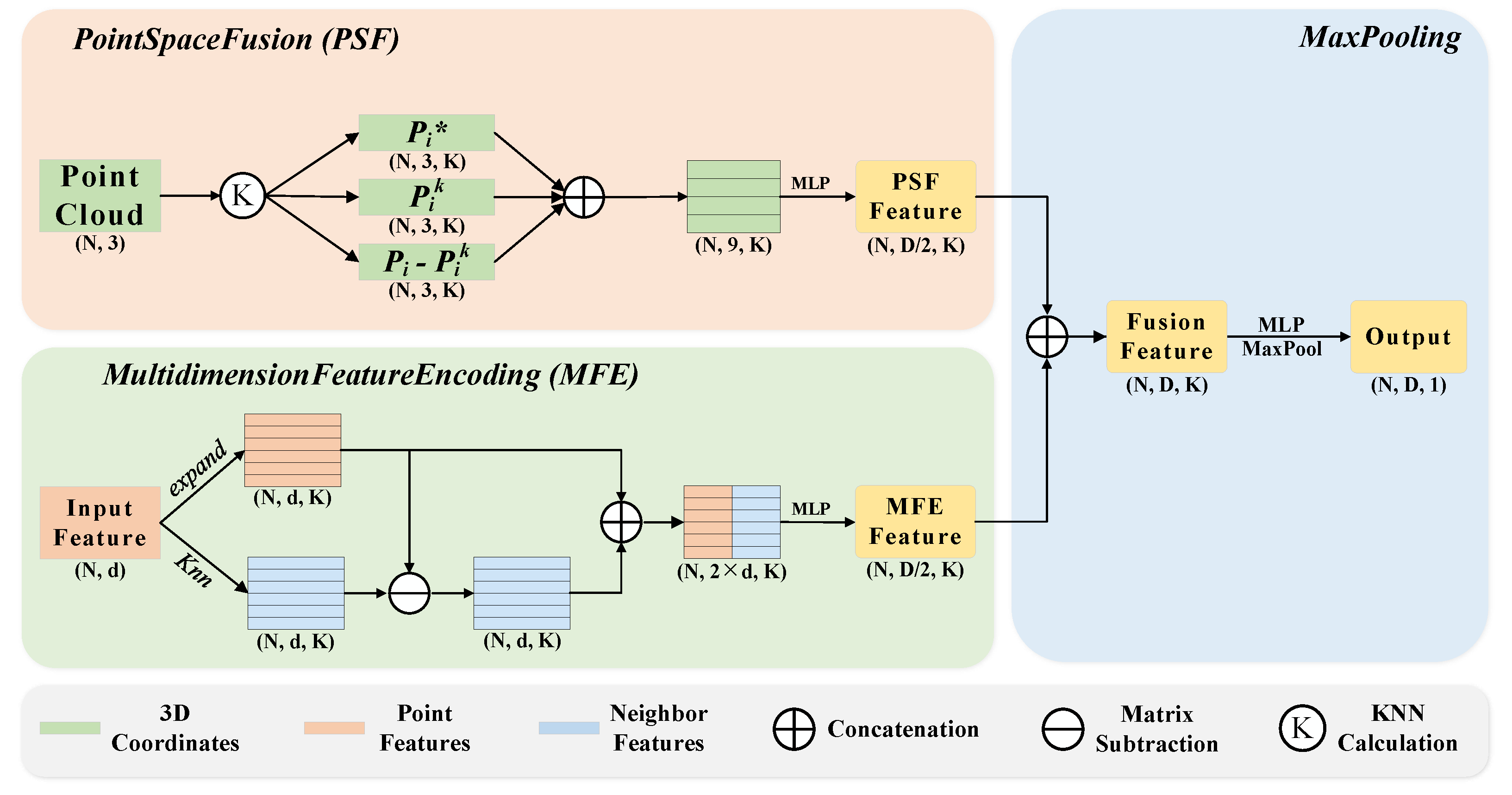
3.2. Feature Extraction Module

During random graph construction it is possible that key points may be dropped, which may cause problems with missing local information. To counter the missing information and extract local significant features, a feature extraction module is proposed to learn the local key features. The designed feature extraction module consists of three neural units: a point space fusion (PSF) unit, multidimension feature encoding (MFE) unit, and max pooling unit (Figure 3).

3.2.1. Point Space Fusion

In this study, the point space fusion (PSF) unit is designed to learn the geometric structure of point clouds from point coordinates and distance information. In recent work, RandLA-Net proposed a random downsampling operation for point cloud semantic segmentation and a local feature aggregation module to alleviate the missing information problem caused by the random downsampling operation. Inspired by RandLA-Net, here, for each point $p_i$ in point cloud P, the spatial information of the nearest K points is fused into the central point $p_i$, ensuring that the context information is gathered together. Specifically, our point space fusion unit is as follows:

(1) Finding neighboring points. For each central point $p_i$, the KNN algorithm is used to find the nearest k points $p_i^1,p_i^2,p_i^3,\dots ,p_i^K$. The KNN algorithm here is based on the Euclidean distance in the 3D space between the central point and its neighboring points.

(2) Calculating distance. For each central point $p_i$ and its nearest k points $\{p_i^1,p_i^2,p_i^3,\dots ,p_i^K\}$ found by the KNN algorithm, the relative distance and absolute distance are calculated as follows:

$$R{D}_i=(p_i-p_i^k),A{D}_i=\left|\right|p_i-p_i^k\left|\right|$$

(2)

where $R{D}_i$ is the relative distance, $A{D}_i$ is the absolute distance, and $\left|\right|\#\left|\right|$ calculates the Euclidean distance in 3D space between the central point and its neighboring points.

(3) Encoding spatial information. For each central point $p_i$ and its nearest k points $\{p_i^1,p_i^2,p_i^3,\dots ,p_i^K\}$, the spatial geometry information is encoded as follows:

$$P_i^k=MLP(p_i\oplus R{D}_i\oplus A{D}_i)$$

(3)

where ⊕ is the concatenation operation and $MLP$ is the multi-layer perceptron. Note that we do not use the absolute distance here, mainly because the calculation of absolute distance consumes more computational resources and these are needed for the graph convolution calculation.

Eventually, a set of spatial information for the point cloud can be obtained as a code of ${\widehat{P}}_i=\{P_i^1,P_i^2,P_i^3,\dots ,P_i^k\}$.

3.2.2. Multidimension Feature Encoding

The multidimensional feature encoding (MFE) unit explicitly encodes the multidimensional features of a point cloud, allowing the network to focus better on the local features. Each point $p_i$ in point cloud P corresponds to feature $f_i$, and the multidimensional feature space F is the set of $f_i$. The MFE unit encodes the local features by the nearest K features for each feature $f_i$ in multidimensional feature space F. Specifically, the MFE unit consists of the following steps:

(1) Finding neighboring features. Unlike the KNN algorithm, which searches for neighboring points based on the Euclidean distance in 3D space, the KNN algorithm used for features is implemented based on the Euclidean distance in multidimensional feature space F. Therefore, for each feature $f_i$ in F, the KNN algorithm is used to search the nearest k features.

(2) Encoding relative features. For each feature $f_i$ and its nearest k features $\{f_i^1,f_i^2,f_i^3,\dots ,f_i^K\}$, the relative features are encoded as follows:

$$F_i^k=MLP((f_i^k\ominus f_i)\oplus f_i)$$

(4)

where ⊖ is the matrix subtraction operation, ⊕ is the concatenation operation, and $MLP$ is the multi-layer perceptron.

Thus, every feature can be encoded. Eventually, the multidimensional feature space can be encoded by the MFE unit using a new set of multidimensional features as ${\widehat{F}}_i=\{F_i^1,F_i^2,F_i^3,\dots ,F_i^k\}$.

3.2.3. Max Pooling

The max pooling unit can extract the most important features in k dimensions. In the max pooling unit, $P_i^k$ and $F_i^k$ are aggregated into a set of local fusion information (${\widehat{F}}_i$). The implementation is as follows:

$$\widehat{F_i}=max\left(MLP(P_i^k\oplus F_i^k)\right)$$

(5)

Eventually, the local fusion information can be encoded by the max pooling unit using a new set of multidimensional features as $\widehat{F_i}$, which can represent the local significant features.

3.3. Network Architecture

In this study, RG-GCN is implemented by stacking multiple Point-GCN (PGCN) modules. The PGCN module consists of the proposed random graph module and the feature extraction module (Figure 4). Figure 4a shows the overall structure of RG-GCN, where the point cloud is input to the network for end-to-end training and the semantic segmentation results are output. Figure 4b shows the PGCN module, which is used to extract the local features of the point cloud.

The PGCN module organically combines the proposed random graph module and the feature extraction module, which can effectively extract the local features of the point cloud. The PGCN module first extracts local significant features using the feature extraction module, then constructs a random graph for the GCN operation.

The network mainly extracts local features with different granularity using multiple PGCN modules and global features using the max pooling layer. The global features and local features are then fused, and the classification score of each point in the point cloud is finally output by MLPs and softmax. The specific details of the network are as follows.

First, a point cloud with dimension $N\times d$ is input to the network (the batch dimension is removed for simplicity), where N is the number of points in the point cloud and d is the initial feature dimension of the input points. The spatial coordinates of the point cloud are used to construct the random graph. The MLP layer, that is, $(d\to 64)$, is used with ReLU and BN to up-dimension the initial features to dimensions $N\times 64$. Then, the features with dimensions $N\times 64$ are treated as the input to four consecutive PGCN modules.

After the features are input to four consecutive PGCN modules, four different levels of cached local features are obtained. All cached local features are concatenated for the MLP layer, that is, $(256\to 1024)$, to obtain features with dimensions $N\times 1024$. Then, they are input to the max pooling layer to obtain a $1\times 1024$ global descriptor.

Subsequently, the 1D global descriptors are extended to each point to obtain $N\times 1024$ global features. The global features and the four previously cached local features are concatenated to obtain fused features which aggregate both global and local features with dimension $N\times (1024+4\times 64)=N\times 1280$.

Finally, three consecutive MLP layers, that is, $(1280\to 512)$, $(512\to 256)$, and $(256\to c)$, are used together with the softmax layer to convert the fused features into label classification scores for each point. The semantic segmentation result is determined by the label with the highest score.

4. Experiments and Discussion

4.1. Experimental Setting

The S3DIS [43] and the Toronto3D [44] datasets were used to fully validate the proposed RG-GCN through experiments. Meanwhile, in order to verify the effect of the network on different numbers of training samples, two experiments were conducted on datasets with sufficient or insufficient training samples. In addition, the effectiveness and rationality of each module were evaluated through ablation studies. Three metrics were used to quantitatively validate the performance of the proposed RG-GCN: intersection over unions (IoUs), mean IoU (mIoU), and overall accuracy (OA), which are defined as follows:

$$\begin{array}{c}\hfill \mathrm{IoU}=\frac{TP}{TP+FP+FN}\end{array}$$

(6)

$$\begin{array}{c}\hfill \mathrm{mIoU}=\frac{{\sum }_{i=1}^n{IoU}_i}{n}\end{array}$$

(7)

$$\begin{array}{c}\hfill \mathrm{OA}=\frac{TP}{N}\end{array}$$

(8)

$$\begin{array}{c}\hfill \mathrm{mAcc}=\frac{\mathrm{OA}}{n}\end{array}$$

(9)

where $TP$ is the number of true positive samples, $FP$ is the number of false positive samples, $FN$ is the number of false negative samples, n is the number of semantic labels, and N is the total number of samples. During the experiments, PyTorch was used to implement RG-GCN. The Adam optimizer used default parameters; the learning rate was initially set to 0.001, the epoch to 100, and the batch size to 12. The random graph module was used to construct the random graph, as described in Section 3.1, where the search range K was set to 25 and the retention rate r to 0.8.

4.2. Indoor Scene Segmentation

The semantic segmentation results of the 3D scene point cloud in the indoor dataset named Stanford 3D Indoor Semantics Dataset (S3DIS) [43] with sufficient or insufficient training samples were used to validate the effectiveness of RG-GCN. In the case with sufficient training samples, RG-GCN achieved 88.1% and 63.7% in OA and mIoU, respectively. In the case with insufficient training samples, RG-GCN achieved 81.1% and 45.8% in OA and mIoU, respectively. These results show that RG-GCN can achieve excellent performance on the indoor dataset.

4.2.1. Dataset Description

The Stanford 3D Indoor Semantics Dataset [43] was collected using a Matterport scanner in six large indoor areas with a total of 272 rooms. The dataset has 13 semantic labels (Figure 5). As with the preprocessing in PointNet [6], in the present study every room was partitioned into blocks of 1 m × 1 m and the point cloud was represented as spatial coordinates ($XYZ$), color information ($RGB$), and normalized spatial coordinates ($X\prime Y\prime Z\prime$).

4.2.2. Results and Visualization with Sufficient Training Samples

In this section, we report the results of the quantitative evaluation of the performance of RG-GCN with sufficient training samples on the S3DIS dataset. Specifically, five of the six areas in the S3DIS were used for training and the remaining one was used for testing. After obtaining the models for the six test areas, six-fold cross-validation was used to evaluate the proposed network.

From the results (

Table 1. Quantitative results of different approaches with sufficient training samples on the S3DIS dataset (six-fold cross-validation).

Method	OA	mIoU	Ceil.	Floor	Wall	Beam	Col.	Wind.	Door	Table	Chair	Sofa	Book.	Board	Clut.
PointNet [6]	78.6	47.6	88.0	88.7	69.3	42.4	23.1	47.5	51.6	54.1	42.0	9.6	38.2	29.4	35.2
RSNet [45]	-	56.5	92.5	92.8	78.6	32.8	34.4	51.6	68.1	59.7	60.1	16.4	50.2	44.9	52.0
3P-RNN [46]	86.9	56.3	92.9	93.8	73.1	42.5	25.9	47.6	59.2	60.4	66.7	24.8	57.0	36.7	51.6
SPG [37]	86.4	62.1	89.9	95.1	76.4	62.8	47.1	55.3	68.4	73.5	69.2	63.2	45.9	8.7	52.9
ShellNet [47]	87.1	66.8	90.2	93.6	79.9	60.4	44.1	64.9	52.9	71.6	84.7	53.8	64.6	48.6	59.4
RandLA-Net [9]	88.0	70.0	93.1	96.1	80.6	62.4	48.0	64.4	69.4	69.4	76.4	60.0	64.2	65.9	60.1
DeepGCNs [12]	85.9	60.0	93.1	95.3	78.2	33.9	37.4	56.1	68.2	64.9	61.0	34.6	51.5	51.1	54.4
DGCNN [8]	84.5	55.5	93.2	95.9	72.8	54.6	32.2	56.2	50.7	62.8	63.4	22.7	38.2	32.5	46.8
RG-GCN (Ours)	88.1	63.7	94.0	96.2	79.1	60.4	44.3	60.1	65.9	70.8	64.9	30.8	51.9	52.6	56.4

), it can be seen that RG-GCN shows excellent performance in terms of OA compared with other methods. With sufficient training samples, RG-GCN achieves 88.1% and 63.7% in OA and mIoU, respectively, which are 3.6% and 7.2% higher than those of DGCNN [8]. The proposed RG-GCN outperforms DGCNN in all 13 labels, mainly because EdgeConv in DGCNN only focuses on the multidimensional features of points without encoding the spatial information. The proposed feature extraction module in RG-GCN aggregates both the spatial information and multidimensional features of the points. Notably, RandLA-Net [9] achieved the best performance in mIoU because it inputs the complete point cloud into the network instead of partitioning the point cloud into blocks, although it takes longer to preprocess the dataset before training.

To compare different methods, this paper visually compares the semantic segmentation results achieved by RG-CCN and DGCNN with sufficient training samples on the S3DIS dataset (Figure 6). From the result, it is visually clear that RG-GCN provides better segmentation of boards and windows compared to DGCNN. In addition, the boundary segmented by DGCNN is not obvious, whereas RG-GCN can segment the boundary of the object more smoothly and accurately. The designed random graph module provides these benefits by randomly constructing an adjacency graph at the beginning of each training epoch. RG-GCN can avoid network underfitting by varying the adjacency graph to learn more features from a small number of labels. This is demonstrated by the objects with a small number of labels in the dataset, such as beams and columns. Meanwhile, for objects with a large number of labels in the dataset, such as the ceiling and floor, RG-GCN can expand the diversity of samples to improve the generalization ability. Moreover, RG-GCN aggregates point spatial information and multidimensional features using the feature extraction module, meaning that the network is able to learn more local significant features.

4.2.3. Results and Visualization with Insufficient Training Samples

In this section, we provide the results of an experiment designed to demonstrate that RG-GCN can achieve state-of-the-art performance even with insufficient training samples. In this experiment, one area in the S3DIS dataset was used for training and the remaining five areas were used for testing. After obtaining the model for the six training areas, six-fold cross-validation was used to evaluate the network. The rest of the setup was the same as for the experiment described in Section 4.2.2.

The results (

Table 2. Quantitative results of different approaches with insufficient training samples on the S3DIS dataset (six-fold cross-validation).

Method	OA	mIoU	Ceil.	Floor	Wall	Beam	Col.	Wind.	Door	Table	Chair	Sofa	Book.	Board	Clut.
PointNet [6]	66.8	31.4	74.6	81.0	56.7	14.5	6.7	17.9	31.9	39.3	28.9	1.7	23.7	8.9	23.1
PointNet++ [7]	75.6	38.8	85.6	90.5	65.9	16.4	6.4	3.4	36.2	55.8	51.9	4.9	35.8	20.8	31.1
DGCNN [8]	76.4	38.3	88.0	89.5	63.8	21.0	12.2	21.2	36.8	50.4	39.6	3.4	29.4	9.5	33.7
KPConv [11]	80.2	43.6	83.8	89.1	65.3	11.0	20.8	27.7	31.5	51.4	52.3	25.3	28.4	40.4	40.0
RandLA-Net [9]	80.5	48.2	88.8	92.0	68.4	28.5	20.2	38.1	44.3	51.8	49.5	25.4	34.8	42.2	42.7
DeepGCNs [12]	78.8	40.4	89.5	90.5	57.5	26.5	19.2	34.9	38.5	52.1	32.1	1.3	32.4	17.4	33.0
RG-GCN (Ours)	81.1	45.8	89.3	92.9	70.1	26.7	13.8	33.6	43.0	57.6	51.1	14.8	37.0	23.6	41.2

) show that when the training samples are insufficient in S3DIS, RG-GCN achieves 81.1% and 45.8% in OA and mIoU, respectively, which is respectively 14.3% and 14.4% higher than PointNet [6] and 4.7% and 7.5% higher than DGCNN [8]. It is clear that RG-GCN has an obvious advantage over the other representative networks when there are insufficient training samples in S3DIS. This is primarily due to the fact that RG-GCN uses a random graph module for effective data augmentation and a feature extraction network to learn local significant features of the point cloud.

This paper visually compares the semantic segmentation results of RG-GCN and DGCNN on the S3DIS dataset with insufficient training samples (Figure 7). Area 3 was selected as the training area for visual comparison analysis because the number of points in Area 3 is the smallest among the six areas, and thus best reflects the training effect with insufficient training samples. From the results, it is clear from the visualization results that both RG-GCN and DGCNN are not visualized as well as the results presented in Section 4.2.2 owing to the insufficiency of the training samples. However, the results of RG-GCN show clear contours, whereas the results of DGCNN show obvious recognition errors in many places and the segmentation boundaries are messy.

4.3. Outdoor Scene Segmentation

The semantic segmentation results of the 3D scene point cloud in the outdoor dataset Toronto3D [44] with sufficient or insufficient training samples were also used to validate the effectiveness of RG-GCN. In the case with sufficient training samples, the RG-GCN network achieved 96.5% and 74.5% in OA and mIoU, respectively. In the case with insufficient training samples, RG-GCN achieved 84.5% and 42.2% in OA and mIoU, respectively. These results show that RG-GCN was able to achieve excellent performance on the outdoor dataset.

4.3.1. Dataset Description

The Toronto3D dataset [44] was obtained using a vehicle-mounted MLS system. The dataset was collected on Avenue Road in Toronto, Canada, covering approximately 1 km of the roadway. The dataset is divided into four areas, each covering approximately 250 m, and is classified into nine semantic labels (Figure 8). During training, each point was only represented as a 6D vector, i.e., spatial coordinates ($XYZ$) and color information ($RGB$).

4.3.2. Results and Visualization with Sufficient Training Samples

In this section, we report the results of the quantitative evaluation of the performance of RG-GCN with sufficient training samples on the Toronto3D dataset. Specifically, following the setup of the Toronto3D dataset, Area 2 was used as the test area to evaluate the performance of the network and the remaining three areas were used as training sets to train the network.

The results quantitatively show the performance of RG-GCN on the Toronto3D dataset compared with other networks (

Table 3. Quantitative results of different approaches with sufficient training samples on the Toronto3D dataset (testing in Area 2).

Method	OA	mIoU	Road	Road mrk.	Nature	Buil.	Util. Line	Pole	Car	Fence
PointNet++ [7]	92.6	59.5	92.9	0.0	86.1	82.2	60.9	62.8	76.4	14.4
MS-PCNN [48]	90.0	65.9	93.8	3.8	93.5	82.6	67.8	71.9	91.1	22.5
TGNet [49]	94.1	61.3	93.5	0.0	90.8	81.6	65.3	62.9	88.7	7.9
MS-TGNet [44]	95.7	70.5	94.4	17.2	95.7	88.8	76.0	73.9	94.2	23.6
DeepGCNs [12]	94.8	67.1	94.2	33.8	91.2	85.3	65.7	62.9	73.6	30.4
KPConv [11]	95.4	69.1	94.6	0.1	96.1	91.5	87.7	81.6	85.7	15.7
RandLA-Net [9]	92.9	77.7	94.6	42.6	96.9	93.0	86.5	78.0	92.9	37.1
DGCNN [8]	94.2	61.7	93.9	0.0	91.3	80.4	62.4	62.3	88.3	15.8
RG-GCN (Ours)	96.5	74.5	98.2	79.4	91.8	86.1	72.4	69.9	82.1	16.0

). RG-GCN outperforms the other networks in terms of OA. With sufficient training samples, RG-GCN achieves 96.5% and 74.5% in OA and mIoU, respectively, which is 2.3% and 12.8% higher than DGCNN [8]. It can be seen that RG-GCN achieves excellent results on ground labels, that is, roads and road markings, whereas most of the other networks are barely able to segment road markings. The best OA that can be achieved is mainly dependent on good segmentation of the ground labels.

As shown in Figure 9, this paper visually compares the semantic segmentation results achieved by RG-CCN and DGCNN on the Toronto3D dataset with sufficient training samples. The first row in Figure 9 shows the overall visualization of Area 2. The second row shows the detailed visualization of part of the crosswalk, which can better display the segmentation results of road markings. The third row shows the visualization of the driving perspective. As highlighted by the red box in Figure 9, it can be seen that most of the labeling results by RG-GCN are consistent with the real situation. Moreover, the proportion of road labels in the Toronto3D dataset is more than half of the total number of labels, and it is easy for the network to misidentify flat surfaces as roads, which is a very challenging problem in the semantic segmentation of outdoor scene data. It can be seen that it is almost impossible for DGCNN to segment road markings; however, the designed RG-GCN has clear segmentation boundaries for road markings, which can better distinguish lane lines and crosswalks.

4.3.3. Results and Visualization with Insufficient Training Samples

In this section, an experiment was designed to demonstrate that RG-GCN can achieve state-of-the-art performance even with insufficient training samples. In this experiment, Area 2, which accounted for 13% of the total area (Figure 8), was used for training and the remaining three areas were used for testing. The rest of the setup was the same as for the experiment described in Section 4.3.2.

The results (

Table 4. Quantitative results of different approaches with insufficient training samples on the Toronto3D dataset (training in Area 2).

Method	OA	mIoU	Road	Road mrk.	Nature	Buil.	Util. Line	Pole	Car	Fence
PointNet [6]	71.6	24.0	79.9	0.4	29.4	63.8	7.1	7.6	3.2	0.7
PointNet++ [7]	77.1	35.2	84.4	0.0	39.2	65.8	29.1	19.3	35.6	8.2
DGCNN [8]	77.8	35.9	82.2	0.6	43.9	63.2	28.9	17.1	43.5	7.8
DeepGCNs [12]	82.2	40.2	86.7	15.8	47.8	66.7	25.5	24.9	41.6	12.4
RandLA-Net [9]	83.8	44.7	88.2	24.5	51.3	74.1	37.0	26.9	40.2	15.5
RG-GCN (Ours)	84.5	43.5	89.9	21.1	45.8	71.2	39.8	24.8	41.2	14.0

) show that when the training samples are insufficient in Toronto3D, RG-GCN achieves 84.5% and 43.5% in OA and mIoU, respectively, which is 7.4% and 8.3% higher than DGCNN [8], respectively. It is clear that in Toronto3D, RG-GCN has an advantage over the other representative networks when the training samples are insufficient.

This research compares the visualization of RG-GCN and DGCNN with inadequate training samples on the Toronto3D dataset (Figure 10). Similar to the image sets in Figure 9, the first row of Figure 10 shows the overall visualization, the second row shows the detailed visualization of part of the crosswalk in order to better display the segmentation results for road markings, and the third row shows the visualization of the driving perspective. DGCNN cannot segment road markings; meanwhile, for the segmentation of cars, DGCNN has multiple obvious segmentation errors, identifying cars as other labels such as roads. In this case, RG-GCN can segment most road markings and cars well, although there is a slight error in the segmentation of edges.

4.4. Ablation Study

4.4.1. Effectiveness and Performance of the Random Graph Module

The threshold (k) for KNN to search neighborhoods for each point and the rate (r) at with the retained neighboring edges are randomly chosen are two important parameters for RG-GCN. The default parameters of RG-GCN were set to $k=25$ and $r=0.8$. To set these parameters appropriately, a grid search method was introduced in the experiments (

Table 5. Comparison of different parameters on the S3DIS dataset (training or testing in Area 6).

Samples	Parameter	OA (%)	mAcc (%)	mIoU (%)	Times (ms)
sufficient	$k=25,r=1.0$	92.1	85.4	76.7	554.7
	$k=25,r=0.9$	92.1	86.5	77.2	520.4
	$k=25,r=0.8$	92.7	87.9	78.4	501.3
	$k=25,r=0.7$	92.5	86.8	77.7	467.6
	$k=25,r=0.6$	91.8	85.0	75.5	445.7
	$k=25,r=0.5$	91.1	83.8	74.3	409.3
	$k=25,r=0.4$	90.6	82.5	72.9	387.1
sufficient	$k=10,r=0.8$	91.8	85.4	75.2	232.8
	$k=15,r=0.8$	92.3	86.9	77.6	326.4
	$k=20,r=0.8$	92.4	87.6	77.9	397.5
	$k=25,r=0.8$	92.7	87.9	78.4	501.3
	$k=30,r=0.8$	92.1	87.1	76.9	592.2
	$k=35,r=0.8$	92.0	86.9	76.4	696.3
	$k=40,r=0.8$	91.8	85.8	75.5	906.3
insufficient	$k=25,r=1.0$	81.1	60.7	48.8	547.4
	$k=25,r=0.9$	81.5	62.1	49.0	511.6
	$k=25,r=0.8$	82.3	62.8	49.9	489.9
	$k=25,r=0.7$	81.8	61.9	49.1	462.3
	$k=25,r=0.6$	80.6	58.7	47.8	439.6
	$k=25,r=0.5$	80.3	58.0	46.9	405.9
	$k=25,r=0.4$	79.8	56.8	46.2	384.9
insufficient	$k=10,r=0.8$	79.7	60.1	46.1	228.4
	$k=15,r=0.8$	80.0	60.7	47.6	323.8
	$k=20,r=0.8$	81.3	61.3	48.5	394.9
	$k=25,r=0.8$	82.3	62.8	49.9	489.9
	$k=30,r=0.8$	81.5	60.6	48.4	594.7
	$k=35,r=0.8$	81.2	60.2	47.9	688.4
	$k=40,r=0.8$	80.6	59.8	47.7	800.2

) and the average computation time for each parameter in computing a batch was compared. From the results, we can see that the OA, mAcc, and mIoU of RG-GCN, where $k=25$ and $r=0.8$, are higher than for the other compared parameters with both sufficient and insufficient training samples. Therefore, the effectiveness of the random graph module is proven.

For the same r and different k, we can see that when $k<25$ the performance of the network improves with an increase in the receptive field, while when $k>25$ the performance of the network decreases with an increase in the receptive field. As a result, it can be concluded that increasing only the receptive field does not improve the performance of the network, and instead may worsen it.

For the same k and different r, it can be seen that when $r>0.8$ the performance of the network improves with a decrease in the randomly retained rate, while when $r<0.8$ the performance of the network weakens with a decrease in the randomly retained rate. As a result, it can be concluded that when the randomly retained rate r is at an appropriate value ($r=0.8$), the network with the added random graph module performs better than the network without the random graph module ($r=1.0$); however, when the random graph module drops too many neighboring edges, too much local information on the point cloud is lost, and the random graph module in this case leads to a decrease in the performance of the network.

4.4.2. Effectiveness of the Feature Extraction Module

In this section, the effectiveness of the feature extraction module is discussed. In order to fairly compare networks with the same number of layers, we replaced the feature extraction module with MLP layers of corresponding sizes, then added ReLU and BN layers after the MLPs. Because MLPs only perform linear affine transformation on the features, it can be considered that MLPs only have the role of dimensional transformation here. Here, we use the S3DIS dataset with training samples that are sufficient or insufficient to experimentally compare non-FEM and RG-GCN.

From the results (

Table 6. Comparison of different parameters on the S3DIS dataset (six-fold cross-validation).

Samples	Parameter	OA (%)	mAcc (%)	mIoU (%)
sufficient	non-FEM	86.4	70.9	60.6
	with-FEM	88.1	74.0	63.7
insufficient	non-FEM	79.5	52.6	42.7
	with-FEM	81.1	56.0	45.8

), it can be seen that the OA, mAcc, and mIoU of RG-GCN with FEM are higher than in the non-FEM case for both the sufficient and insufficient training sample scenarios. Compared with MLPs, with only linear affine transformation of the features, the proposed feature extraction module can encode local significant features by aggregating point spatial information and multidimensional features. The point space fusion unit aggregates the coordinates of the point and the nearest points along with the relative and absolute distances between them, which can better extract the spatial geometric structure of the point cloud. The multidimensional feature encoding unit aggregates the feature and its nearest features, which can better represent the local neighborhood features. Thus, the feature extraction module enables the network to learn local significant features in the training samples.

4.4.3. Exploration of the Number of PGCN Modules

In this section, we compare the performance of RG-GCN when different numbers of PGCN modules are used. Our RG-GCN uses four consecutive PGCN modules to extract features from the point cloud. Here, using the S3DIS dataset with sufficient or insufficient training samples, different numbers of PGCN modulesare are treated as a comparative experiment.

From the results (Figure 11), it can be seen that four consecutive PGCN modules perform the best, and provide superior performance on OA and mIoU over other numbers of PGCN modules. When the number of PGCN modules is less than four, the performance of the network increases as the number of modules increases. This is because as the number of PGCN modules increases the network can more efficiently learn more local features and geometric information. When the number of PGCN modules is greater than five, the performance of the network decreases. This is mainly because too many PGCN modules leads to overfitting of the network, meaning that the network focuses too much on local features while overlooking global features.

5. Conclusions

Semantic segmentation is widely used and is a challenging task in 3D point cloud research. In this study, a graph-based network for point cloud semantic segmentation is proposed which can achieve better results than currently used methods when the training sample is sufficient. At the same time, it provides improved performance when the training sample is insufficient. In this network, a random graph module and a feature extraction module are designed to improve the performance of semantic segmentation. The proposed random graph module performs data augmentation by changing the topology of the built graphs, which does not require additional expansion of the training samples. The proposed feature extraction module is designed to learn the local significant features of a point cloud, and can effectively aggregate point spatial information and multidimensional features. Based on the random graph module and feature extraction module, this paper proposes an end-to-end network called RG-GCN. Validation experiments show that the proposed network effectively achieves excellent performance for point cloud semantic segmentation with both sufficient and insufficient training samples.

However, the point cloud input to the network is not complete data, and is partitioned into blocks. The network can learn only the features within a block, and the receptive field is confined. Moreover, cutting the entire point cloud into blocks results in the loss of the overall geometric structure. In future works, we aim to improve the network framework to use the complete 3D scene point cloud instead of partitioned blocks, thereby improving the input to the network.

References

1. Endres, F.; Hess, J.; Sturm, J.; Cremers, D.; Burgard, W. 3-D Mapping With an RGB-D Camera. IEEE Trans. Robot. 2014, 30, 177–187. [Google Scholar] [CrossRef]
2. Jaboyedoff, M.; Oppikofer, T.; Abellán, A.; Derron, M.H.; Loye, A.; Metzger, R.; Pedrazzini, A. Use of LIDAR in landslide investigations: A review. Nat. Hazards 2012, 61, 5–28. [Google Scholar] [CrossRef]
3. Guo, Y.; Wang, H.; Hu, Q.; Liu, H.; Liu, L.; Bennamoun, M. Deep Learning for 3D Point Clouds: A Survey. IEEE Trans. Pattern Anal. Mach. Intell. 2021, 43, 4338–4364. [Google Scholar] [CrossRef] [PubMed]
4. Zeng, Z.; Xu, Y.; Xie, Z.; Tang, W.; Wan, J.; Wu, W. LEARD-Net: Semantic Segmentation for Large-Scale Point Cloud Scene. Int. J. Appl. Earth Obs. Geoinf. 2022, 112, 102953. [Google Scholar] [CrossRef]
5. Han, X.; Dong, Z.; Yang, B. A point-based deep learning network for semantic segmentation of MLS point clouds. Isprs J. Photogramm. Remote. Sens. 2021, 175, 199–214. [Google Scholar] [CrossRef]
6. Charles, R.Q.; Su, H.; Kaichun, M.; Guibas, L.J. PointNet: Deep Learning on Point Sets for 3D Classification and Segmentation. In Proceedings of the IEEE Conference on Computer Vision and Pattern Recognition (CVPR), Honolulu, HI, USA, 21–26 July 2017. [Google Scholar]
7. Qi, C.R.; Yi, L.; Su, H.; Guibas, L.J. PointNet++: Deep Hierarchical Feature Learning on Point Sets in a Metric Space. In Proceedings of the 31st Conference on Neural Information Processing Systems (NIPS 2017), Long Beach, CA, USA, 4–9 December 2017. [Google Scholar]
8. Wang, Y.; Sun, Y.; Liu, Z.; Sarma, S.E.; Bronstein, M.M.; Solomon, J.M. Dynamic Graph CNN for Learning on Point Clouds. ACM Trans. Graph 2019, 38, 146. [Google Scholar] [CrossRef]
9. Hu, Q.; Yang, B.; Xie, L.; Rosa, S.; Guo, Y.; Wang, Z.; Trigoni, N.; Markham, A. RandLA-Net: Efficient Semantic Segmentation of Large-Scale Point Clouds. In Proceedings of the IEEE/CVF Conference on Computer Vision and Pattern Recognition (CVPR), Seattle, WA, USA, 13–19 June 2020. [Google Scholar]
10. Wang, L.; Huang, Y.; Hou, Y.; Zhang, S.; Shan, J. Graph Attention Convolution for Point Cloud Semantic Segmentation. In Proceedings of the IEEE/CVF Conference on Computer Vision and Pattern Recognition (CVPR), Long Beach, CA, USA, 15–20 June 2019. [Google Scholar]
11. Thomas, H.; Qi, C.R.; Deschaud, J.-E.; Marcotegui, B.; Goulette, F.; Guibas, L.J. KPConv: Flexible and Deformable Convolution for Point Clouds. In Proceedings of the IEEE/CVF International Conference on Computer Vision (ICCV), Seoul, Korea, 27 October–2 November 2019. [Google Scholar]
12. Li, G.; Müller, M.; Thabet, A.; Ghanem, B. DeepGCNs: Can GCNs Go As Deep As CNNs? In Proceedings of the IEEE/CVF International Conference on Computer Vision (ICCV), Seoul, Korea, 27 October–2 November 2019. [Google Scholar]
13. Hu, B.; Xu, Y.; Wan, B.; Wu, X.; Yi, G. Hydrothermally altered mineral mapping using synthetic application of Sentinel-2A MSI, ASTER and Hyperion data in the Duolong area, Tibetan Plateau, China. Ore Geol. Rev. 2018, 101, 384–397. [Google Scholar] [CrossRef]
14. Hu, B.; Wan, B.; Xu, Y.; Tao, L.; Wu, X.; Qiu, Q.; Wu, Y.; Deng, H. Mapping hydrothermally altered minerals with AST_07XT, AST_05 and Hyperion datasets using a voting-based extreme learning machine algorithm. Ore Geol. Rev. 2019, 114, 103116. [Google Scholar] [CrossRef]
15. Hu, B.; Xu, Y.; Huang, X.; Cheng, Q.; Ding, Q.; Bai, L.; Li, Y. Improving Urban Land Cover Classification with Combined Use of Sentinel-2 and Sentinel-1 Imagery. ISPRS Int. J. Geo-Inf. 2021, 10, 533. [Google Scholar] [CrossRef]
16. Xu, Y.; He, Z.; Xie, X.; Xie, Z.; Luo, J.; Xie, H. Building function classification in Nanjing, China, using deep learning. Trans. Gis 2022, 26, 2145–2165. [Google Scholar] [CrossRef]
17. Zou, L.; Tang, H.; Chen, K.; Jia, K. Geometry-Aware Self-Training for Unsupervised Domain Adaptation on Object Point Clouds. In Proceedings of the IEEE/CVF International Conference on Computer Vision (ICCV), Montreal, BC, Canada, 11–17 October 2021. [Google Scholar]
18. Poursaeed, O.; Jiang, T.; Qiao, H.; Xu, N.; Kim, V.G. Self-Supervised Learning of Point Clouds via Orientation Estimation. In Proceedings of the International Conference on 3D Vision (3DV), Fukuoka, Japan, 25–28 November 2020. [Google Scholar]
19. Shorten, C.; Khoshgoftaar, T. A survey on Image Data Augmentation for Deep Learning. J. Big Data 2019, 6, 60. [Google Scholar] [CrossRef]
20. Xu, Y.; Jin, S.; Chen, Z.; Xie, X.; Hu, S.; Xie, Z. Application of a graph convolutional network with visual and semantic features to classify urban scenes. Int. J. Geogr. Inf. Sci. 2022, 1–26. [Google Scholar] [CrossRef]
21. Yun, S.; Han, D.; Chun, S.; Oh, S.J.; Yoo, Y. CutMix: Regularization Strategy to Train Strong Classifiers With Localizable Features. In Proceedings of the IEEE/CVF International Conference on Computer Vision (ICCV), Seoul, Korea, 27 October–2 November 2019. [Google Scholar]
22. Zhao, N.; Chua, T.S.; Lee, G.H. Few-shot 3d point cloud semantic segmentation. In Proceedings of the IEEE Conference on Computer Vision and Pattern Recognition (CVPR), Nashville, TN, USA, 20–25 June 2021. [Google Scholar]
23. Li, R.; Li, X.; Heng, P.-A.; Fu, C.-W. PointAugment: An Auto-Augmentation Framework for Point Cloud Classification. In Proceedings of the IEEE/CVF Conference on Computer Vision and Pattern Recognition (CVPR), Seattle, WA, USA, 13–19 June 2020. [Google Scholar]
24. Goodfellow, I.J.; Pouget-Abadie, J.; Mirza, M.; Xu, B.; Warde-Farley, D.; Ozair, S.; Courville, A.; Bengio, Y. Generative Adversarial Nets. In Proceedings of the Advances in Neural Information Processing Systems, Montreal, QC, Candad, 8–13 December 2014. [Google Scholar]
25. Zhou, J.; Shen, J.; Yu, S.; Chen, G.; Xuan, Q. M-Evolve: Structural-Mapping-Based Data Augmentation for Graph Classification. IEEE Trans. Netw. Sci. Eng. 2021, 8, 190–200. [Google Scholar] [CrossRef]
26. Wu, W.; Xie, Z.; Xu, Y.; Zeng, Z.; Wan, J. Point Projection Network: A Multi-View-Based Point Completion Network with Encoder-Decoder Architecture. Remote. Sens. 2021, 13, 4917. [Google Scholar] [CrossRef]
27. Chen, X.; Ma, H.; Wan, J.; Li, B.; Xia, T. Multi-view 3D Object Detection Network for Autonomous Driving. In Proceedings of the IEEE/CVF Conference on Computer Vision and Pattern Recognition (CVPR), Honolulu, HI, USA, 21–26 July 2017. [Google Scholar]
28. Lang, A.H.; Vora, S.; Caesar, H.; Zhou, L.; Yang, J.; Beijbom, O. PointPillars: Fast Encoders for Object Detection From Point Clouds. In Proceedings of the IEEE/CVF Conference on Computer Vision and Pattern Recognition (CVPR), Long Beach, CA, USA, 15–20 June 2019. [Google Scholar]
29. Yu, T.; Meng, J.; Yuan, J. Multi-view Harmonized Bilinear Network for 3D Object Recognition. In Proceedings of the IEEE/CVF Conference on Computer Vision and Pattern Recognition (CVPR), Salt Lake City, UT, USA, 18–22 June 2018. [Google Scholar]
30. Le, T.; Duan, Y. PointGrid: A Deep Network for 3D Shape Understanding. In Proceedings of the IEEE/CVF Conference on Computer Vision and Pattern Recognition (CVPR), Salt Lake City, UT, USA, 18–22 June 2018. [Google Scholar]
31. Graham, B.; Engelcke, M.; van der Maaten, L. 3D Semantic Segmentation with Submanifold Sparse Convolutional Networks. In Proceedings of the IEEE/CVF Conference on Computer Vision and Pattern Recognition (CVPR), Salt Lake City, UT, USA, 18–22 June 2018. [Google Scholar]
32. Maturana, D.; Scherer, S. VoxNet: A 3D Convolutional Neural Network for real-time object recognition. In Proceedings of the IEEE/RSJ International Conference on Intelligent Robots and Systems (IROS), Hamburg, Germany, 28 September–3 October 2015. [Google Scholar]
33. Wan, J.; Xie, Z.; Xu, Y.; Zeng, Z.; Yuan, D.; Qiu, Q. DGANet: A Dilated Graph Attention-Based Network for Local Feature Extraction on 3D Point Clouds. Remote. Sens. 2021, 13, 3484. [Google Scholar] [CrossRef]
34. Xu, Q.; Sun, X.; Wu, C.-Y.; Wang, P.; Neumann, U. Grid-GCN for Fast and Scalable Point Cloud Learning. In Proceedings of the IEEE/CVF Conference on Computer Vision and Pattern Recognition (CVPR), Seattle, WA, USA, 14–19 June 2020. [Google Scholar]
35. Liu, J.; Ni, B.; Li, C.; Yang, J.; Tian, Q. Dynamic Points Agglomeration for Hierarchical Point Sets Learning. In Proceedings of the IEEE/CVF International Conference on Computer Vision (ICCV), Seoul, Korea, 27 October–2 November 2019. [Google Scholar]
36. Landrieu, L.; Boussaha, M. Point Cloud Oversegmentation With Graph-Structured Deep Metric Learning. In Proceedings of the IEEE/CVF Conference on Computer Vision and Pattern Recognition (CVPR), Long Beach, CA, USA, 15–20 June 2019. [Google Scholar]
37. Landrieu, L.; Simonovsky, M. Large-Scale Point Cloud Semantic Segmentation with Superpoint Graphs. In Proceedings of the IEEE/CVF Conference on Computer Vision and Pattern Recognition, Salt Lake City, UT, USA, 18–22 June 2018. [Google Scholar]
38. Tran, T.; Pham, T.; Carneiro, G.; Palmer, L.; Reid, I. A Bayesian Data Augmentation Approach for Learning Deep Models. In Proceedings of the Neural Information Processing Systems, Long Beach, CA, USA, 4–9 December 2017. [Google Scholar]
39. Lemley, J.; Bazrafkan, S.; Corcoran, P. Smart Augmentation Learning an Optimal Data Augmentation Strategy. IEEE Access 2017, 5, 5858–5869. [Google Scholar] [CrossRef]
40. Shrivastava, A.; Pfister, T.; Tuzel, O.; Susskind, J.; Wang, W.; Webb, R. Learning from Simulated and Unsupervised Images through Adversarial Training. In Proceedings of the IEEE Conference on Computer Vision and Pattern Recognition (CVPR), Honolulu, HI, USA, 21–26 July 2017. [Google Scholar]
41. You, Y.; Chen, T.; Sui, Y.; Chen, T.; Wang, Z.; Shen, Y. Graph Contrastive Learning with Augmentations. In Proceedings of the Neural Information Processing Systems, online, 6–12 December 2020. [Google Scholar]
42. Tang, Z.; Qiao, Z.; Hong, X.; Wang, Y.; Dharejo, F.A.; Zhou, Y.; Du, Y. Data Augmentation for Graph Convolutional Network on Semi-Supervised Classification. In Proceedings of the Web and Big Data, Guangzhou, China, 23–25 August 2021. [Google Scholar]
43. Armeni, I.; Sener, O.; Zamir, A.R.; Jiang, H.; Brilakis, I.; Fische, M.; Savares, S. 3D Semantic Parsing of Large-Scale Indoor Spaces. In Proceedings of the IEEE Conference on Computer Vision and Pattern Recognition (CVPR), Las Vegas, NV, USA, 27–30 June 2016. [Google Scholar]
44. Tan, W.; Qin, N.; Ma, L.; Li, Y.; Du, J.; Cai, G.; Yang, K.; Li, J. Toronto-3D: A Large-scale Mobile LiDAR Dataset for Semantic Segmentation of Urban Roadways. In Proceedings of the IEEE/CVF Conference on Computer Vision and Pattern Recognition Workshops (CVPRW), Seattle, WA, USA, 14–19 June 2020. [Google Scholar]
45. Huang, Q.; Wang, W.; Neumann, U. Recurrent Slice Networks for 3D Segmentation of Point Clouds. In Proceedings of the IEEE/CVF Conference on Computer Vision and Pattern Recognition, Salt Lake City, UT, USA, 18–22 June 2018. [Google Scholar]
46. Ye, X.; Li, J.; Huang, H.; Du, L.; Zhang, X. 3D Recurrent Neural Networks with Context Fusion for Point Cloud Semantic Segmentation. In Proceedings of the Computer Vision—ECCV, Munich, Germany, 8–14 September 2018. [Google Scholar]
47. Zhang, Z.; Hua, B.-S.; Yeung, S.-K. ShellNet: Efficient Point Cloud Convolutional Neural Networks Using Concentric Shells Statistics. In Proceedings of the IEEE/CVF International Conference on Computer Vision (ICCV), Seoul, Korea, 27 October–2 November 2019. [Google Scholar]
48. Ma, L.; Li, Y.; Li, J.; Tan, W.; Yu, Y.; Chapman, M.A. Multi-Scale Point-Wise Convolutional Neural Networks for 3D Object Segmentation From LiDAR Point Clouds in Large-Scale Environments. IEEE Trans. Intell. Transp. Syst. 2021, 22, 821–836. [Google Scholar] [CrossRef]
49. Li, Y.; Ma, L.; Zhong, Z.; Cao, D.; Li, J. TGNet: Geometric Graph CNN on 3-D Point Cloud Segmentation. IEEE Trans. Geosci. Remote. Sens. 2020, 58, 3588–3600. [Google Scholar] [CrossRef]
Figure 1. Proposed random graph module: (a) input point cloud, (b) KNN algorithm to construct adjacency graphs, and (c) random graph module to construct different random graphs.
Remotesensing 14 04055 g001
Figure 2. Comparison of adjacency graphs and random graph: (a) adjacency graph with K = 6 , (b) adjacency graph with K = 12 , and (c) random graph with K = 12 and r = 0.5 .
Remotesensing 14 04055 g002
Figure 3. Proposed feature extraction module: the top left panel shows the PSF unit, the bottom left panel shows the MFE unit, and the right panel shows the max pooling unit.
Remotesensing 14 04055 g003
Figure 4. Overall structure of the proposed network and the PGCN module: (a) overall structure of RG-GCN and (b) PGCN module.
Remotesensing 14 04055 g004
Figure 5. Proportion of areas and labels in the S3DIS dataset: (a) proportion of six areas, (b) the main proportion of 13 labels, and (c) the remaining proportion of 13 labels.
Remotesensing 14 04055 g005
Figure 6. Visual comparison onf S3DIS dataset with sufficient training samples: (a) ground truth labels, (b) results of proposed RG-GCN, and (c) results of DGCNN.
Remotesensing 14 04055 g006
Figure 7. Visual comparison on S3DIS dataset with insufficient training samples: (a) ground truth labels, (b) results of our RG-GCN, and (c) results of DGCNN.
Remotesensing 14 04055 g007
Figure 8. Proportion of areas and labels in Toronto3D dataset: (a) the proportion of the four areas, (b) the main proportion of the eight labels, and (c) the rest of the proportion of the eight labels.
Remotesensing 14 04055 g008
Figure 9. Visual comparison on Toronto3D dataset with sufficient training samples: (a) full RGB, (b) ground truth labels, (c) results with our RG-GCN, and (d) results with DGCNN.
Remotesensing 14 04055 g009
Figure 10. Visual comparison on Toronto3D dataset with insufficient training samples: (a) full RGB, (b) ground truth labels, (c) results with our RG-GCN, and (d) results with DGCNN.
Remotesensing 14 04055 g010
Figure 11. Comparison of different numbers of PGCN modules on the S3DIS dataset (six-fold cross-validation). (a) sufficient training samples. (b) insufficient training samples.
Remotesensing 14 04055 g011