Article

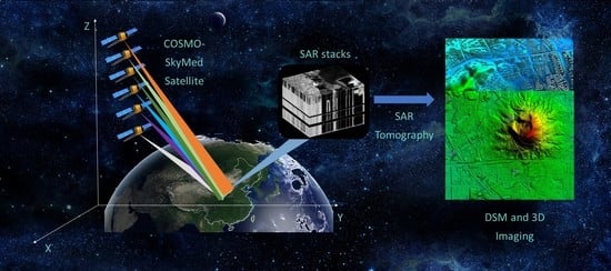
Elevation Extraction from Spaceborne SAR Tomography Using Multi-Baseline COSMO-SkyMed SAR Data

1
Imaging Group, Mullard Space Science Laboratory (MSSL), Department of Space & Climate Physics, University College London, Holmbury St Mary RH5 6NT, UK
2
Hiwing Satellite Operation Division of China Aerospace Science and Industry Corporation, Beijing 100070, China
3
Department of Geospatial Information, PLA Strategic Support Force Information Engineering University, Zhengzhou 450052, China
4
Institute of Crustal Dynamics, China Earthquake Administration, Beijing 100085, China
*
Author to whom correspondence should be addressed.
Remote Sens. 2022, 14(16), 4093; https://doi.org/10.3390/rs14164093
Submission received: 29 June 2022 / Revised: 9 August 2022 / Accepted: 19 August 2022 / Published: 21 August 2022
(This article belongs to the Special Issue Recent Progress and Applications on Multi-Dimensional SAR)

Abstract

:
SAR tomography (TomoSAR) extends SAR interferometry (InSAR) to image a complex 3D scene with multiple scatterers within the same SAR cell. The phase calibration method and the super-resolution reconstruction method play a crucial role in 3D TomoSAR imaging from multi-baseline SAR stacks, and they both influence the accuracy of the 3D SAR tomographic imaging results. This paper presents a systematic processing method for 3D SAR tomography imaging. Moreover, with the newly released TanDEM-X 12 m DEM, this study proposes a new phase calibration method based on SAR InSAR and DEM error estimation with the super-resolution reconstruction compressive sensing (CS) method for 3D TomoSAR imaging using COSMO-SkyMed Spaceborne SAR data. The test, fieldwork, and results validation were executed at Zipingpu Dam, Dujiangyan, Sichuan, China. After processing, the 1 m resolution TomoSAR elevation extraction results were obtained. Against the terrestrial Lidar ‘truth’ data, the elevation results were shown to have an accuracy of 0.25 ± 1.04 m and a RMSE of 1.07 m in the dam area. The results and their subsequent validation demonstrate that the X band data using the CS method are not suitable for forest structure reconstruction, but are fit for purpose for the elevation extraction of manufactured facilities including buildings in the urban area.

Graphical Abstract

1. Introduction

3D SAR tomography (TomoSAR) [1,2,3,4] and its closely associated 4D SAR differential tomography (Diff-TomoSAR) [5,6,7,8,9] take advantage of multi-baseline SAR data stacks to create an important innovation in SAR interferometry, allowing for the sensing of complex scenes with multiple scatterers mapped into the same SAR cell. The idea of tomographic imaging was first introduced to the field of SAR research in the 1990s [10,11,12] in order to overcome the limitations (e.g., 3D information extraction) of 2D SAR imaging. The initial experiment was carried out in a laboratory under ideal experimental conditions [13] and subsequently by using airborne systems [1]. In 2010, researchers such as Zhu and Bamler of the DLR Laboratory in Germany used a tomographic SAR inversion method based on L1 norm compression sensing to separate scattering particles distributed along the vertical dimension within the same cell using spaceborne SAR data. Subsequently, this method has been applied to 3D ultra-high-resolution tomographic SAR imaging in complex urban environments, while the compressive sensing method based on the L1 norm has also been applied to differential tomography SAR [14,15,16]. In this way, classical 2D InSAR can be considered as a simple parametric case of 3D TomoSAR. D-TomoSAR (4D SAR imaging) [6,16,17] exploits the strengths of both TomoSAR and PSI, which inverts the motion of the scatterers with 3D TomoSAR reconstruction [16], which can retrieve the motion [18,19] and elevation information of multiple scatterers in a SAR pixel cell using a spectral analysis method [20]. In addition to 3D shape reconstruction, they permit a solution for monitoring deformation in complex urban/infrastructure areas [2,4] as well as recent cryospheric ice investigations [21], emerging tomographic remote sensing applications including forest scenarios [3,22,23] (e.g., tree height and biomass estimation), sub-canopy topographic mapping, and even search, rescue, and surveillance applications under forest.
However, these scenes are characterized and influenced by DEM uncertainty, the temporal decorrelation of scatterers, orbital, tropospheric and ionospheric phase distortion, and an open issue regarding possible height blurring and accuracy losses for TomoSAR applications, particularly in densely vegetated mountainous rural areas and polar icy regions of the Earth, alongside the polar region of many planets (the Moon, Mars, and Mercury) and their icy satellites (moons) such as Europa, Ganymede, Callisto, and so on. To address the problems inherent in these techniques, baseline estimation should be conducted in advance and phase calibration is critical and indispensable in 3D SAR tomographic imaging. Here, COSMO-SkyMed spaceborne SAR data were applied to various applications in the world. Currently, there have only been rare reports on TomoSAR applications using these particular SAR satellite data. This paper presents a systematic processing method for 3D SAR tomography imaging using COSMO-SkyMed spaceborne SAR. In addition, a new phase calibration method is presented based on SAR interferometry (InSAR) and DEM error estimation, and compensation with the newly released geographically extremely limited areas of TanDEM-X 12 m DEM for 3D TomoSAR imaging is also shown. The test, fieldwork, results validation, new method discussion, CS algorithm adaptability analysis, and results analysis were conducted at Zipingpu Dam, Dujiangyan, Sichuan, China. In Section 2.1, the mathematical principles are described, whilst in Section 2.2, the SAR interferometry phase (InSAR) calibration with the DEM error is described. In Section 3, the results are shown for the dam test site whereas in Section 4, these are discussed and our conclusions are presented in the final section.

2. Methodology

2.1. Principles

The two-dimensional imaging principle for SAR assumes that the target is a two-dimensional plane target, while the actual target exists in a three-dimensional space. Two-dimensional SAR imaging results from the projection of the three-dimensional structure and targets into a two-dimensional plane (azimuth-range plane). Three-dimensional space is divided into a series of equidistant cylindrical surfaces along the azimuth axis, but SAR fails to distinguish targets on the same cylindrical surface because these targets are compressed into the same pixel at the same distance. This is the cylindrical symmetric ambiguity problem in SAR two-dimensional imaging. Since high azimuth resolution imaging can be obtained by the synthesis aperture method using a small sized radar antenna, two-dimensional high-resolution imaging in the elevation plane can be realized if a two-dimensional synthetic aperture is formed in the elevation direction with the help of high-resolution range direction imaging to achieve a true three-dimensional radar imaging. This is the basic idea of three-dimensional SAR imaging, TomoSAR. A normal monostatic imaging SAR system consists of a side-looking transmitter and receiver mounted on a moving platform such as an airplane or satellite. TomoSAR builds up a synthetic elevation aperture from a stack of N complex SAR datasets of the same area taken at different times and slightly different orbit positions. The native 3D reference frame of a SAR sensor and the parameters of SAR maps in the three directions are defined as below (x azimuth, r range, s elevation), which is displayed in the TomoSAR imaging geometry in Figure 1. According to previous research [1,2,3,4], the workflow of SAR tomography and D-TomoSAR is shown in Figure 2. First, all complex images were co-registered into SAR stacks. Then, the atmospheric and ionospheric corrections were performed. Next, deramping and phase error compensation were executed. Finally, the results can be obtained after 3D TomoSAR imaging and post-processing.
Theoretically, the range-azimuth resolution cell in a sequence of images ( M images) corresponds to the same feature with pixels indexed by ( s ), and its complex image single-look-complex (SLC) value Q ( m ) which can be written as below [2,24],
Q ( m ) = s m i n s m a x   γ ( s ) e x p ( j 4 π f 0 c R m ( s ) ) d s ,   m = 1 , 2 , , M ,
where γ ( s ) refers to the complex scattering coefficient; s represents the elevation; f 0 is the frequency; c is the speed of light; and R m ( s ) is the slant range. After removing the phase term caused by the reference slant range R m ( 0 ) at the phase center of each image, called deramping [2,24], the mth image can be written as g ( m ) .
g ( m ) = e x p ( j 4 π f 0 c R m ( 0 ) ) Q ( m ) ,   = s m i n s m a x γ ( s ) e x p ( j 4 π f 0 c ( R m ( s ) R m ( 0 ) ) ) d s ,
After calculation and simplification [2,25], Equation (2) be expressed in the following form,
g ( m ) = s m i n s m a x γ ( s ) e x p ( j 2 π ξ m s ) d s ,
ξ m = 2 b m λ r ,
where ξ m is the spatial frequency corresponding to the height s from the normal slant-range direction (NSR direction or here called s , elevation direction), and b m refers to the perpendicular baseline. As seen from Equation (3), the complex values g ( m ) , m = 1 , 2 , , M are the target discrete cell samples of electromagnetic scattering characteristics γ ( s ) along the NSR direction at ξ m after SLC image deramping. In other words, SAR tomographic imaging is essentially the use of spectral discrete sampling reconstruction of the original signal problem, and it is necessary to obtain the spatial frequency ξ m first.
Based on Equation (2), the deramping operation plays a critical role in SAR tomography. It is precisely because of the removal of the central slant phase that the intrinsic relationship between the observed data and the target NSR information is established.
The reference slant range used in the deramping step can be obtained in two ways: (1) calculating the reference slant range using the radar transmission center time delay and velocity recorded by the radar; and (2) calculating the reference slant range based on some reference topography and radar position [1,2,3,4]. The reference slant range used in the deramping can be the center distance of each image, or the distance between the radar antenna phase center of each image and a reference terrain (e.g., known coarse resolution DEM data). Although the most direct deramping method is to remove the slant range to the phase center via the radar-recorded electromagnetic propagation delay, the use of its deramping introduces additional atmospheric phase errors because the echo delay is affected by atmospheric interference, which also needs to use an offset co-registration interpolation method to calculate the reference slant range. A reference terrain is more commonly used because it only requires the calculation of the reference slant range based on the radar position and the terrain [24,26]. Therefore, a coarse DEM is generally applied via flattening of the simulated phase by a DEM. In addition, for scenes with lower relief, one can also use ellipse models that have been improved based on the average elevation of the scene [24,26]. According to previous research [27], the phase simulation by DEM is expressed as:
φ s i m u _ m = 4 π λ b m ,
where b m is the parallel baseline; therefore, according to Equation (5), it can be observed that parallel baseline estimation is extremely important for TomoSAR deramping. Considering that the parallel baseline estimation is common in InSAR [28,29,30], it is not described here because this is not the key point of this study.
As noted in InSAR [28,29,30], the InSAR calculation method (interferometry and then flattening) is shown in Equation (6). I m a s t is the master SLC data; I s l a v e is the slave SLC data; ( )   * means the conjugated calculation. In this way, we define that SLC data ( I ) are flattened, followed by Equation (7), which is the basic processing operation in software codes in many InSAR software.
{ I m a s t · ( I s l a v e ) * } f l a t t e n i n g = I m a s t · ( I s l a v e ) * ·   e x p ( j · φ s i m u m   ) = I m a s t · (   I s l a v e · e x p ( j · φ s i m u m   )   ) * ,
{ I s l a v e } f l a t t e n i n g = I s l a v e · e x p ( j · φ s i m u _ m )   ,
If Equation (2) is multiplied by e x p ( j 4 π λ R ) , R is the central phase slant range of the master image, then Equation (2) becomes Equation (8).
p ( ξ m ) = e x p ( j 4 π λ R ) . g ( m ) = e x p ( j 4 π λ R ) e x p ( j 4 π f 0 c R m ( 0 ) ) Q ( m ) = e x p ( j · 4 π λ [ R R m ( 0 ) ] ) ·   Q ( m ) ,
From Equation (2), Rm(0) is the central slant range of each image (slave image) and if φ m is defined as
φ m = 4 π λ [ R R m ( 0 ) ] ,
Equation (2) becomes Equation (10).
p ( ξ m ) = e x p ( j ·   φ m ) ·   Q ( m ) ,
It can be seen that φ m is the interferometric phase. If the DEM error is ignored and φ m is replaced by the DEM simulation phase, Equation (10) is identical to Equation (7). This is because Q ( m ) = I ( m ) , and they are all the same (mth) SLC data. In this way, based on Equation (2), the flattening of the SLC data ( I f l a t t e n i n g ) is shown in Equation (11).
I f l a t t e n i n g ( m ) = I ( m ) · e x p ( j · φ s i m u _ m ) = Q ( m ) · e x p ( j · φ s i m u _ m ) = e x p ( j · φ s i m u _ m ) ·   Q ( m ) = p ( ξ m ) = e x p ( j 4 π λ R ) g ( m ) = s m i n s m a x e x p ( j 4 π λ R ) γ ( s ) e x p ( j 2 π ξ m s ) d s ,
If γ ( s ) is defined in Equation (12), the flattening of the SLC data in Equation (11) becomes Equation (13). Therefore, the flattening of SLC data ( I f l a t t e n i n g ) can be directly used in TomoSAR processing, followed by the use of core Equations (8)–(13). γ ( s ) is the inversion results of TomoSAR processing along the s direction (NSR direction).
γ ( s ) = e x p ( j   4 π λ R )   γ ( s ) ,
I f l a t t e n i n g ( m ) = p ( ξ m ) = s m i n s m a x γ ( s )   e x p ( j 2 π ξ m s ) d s ,

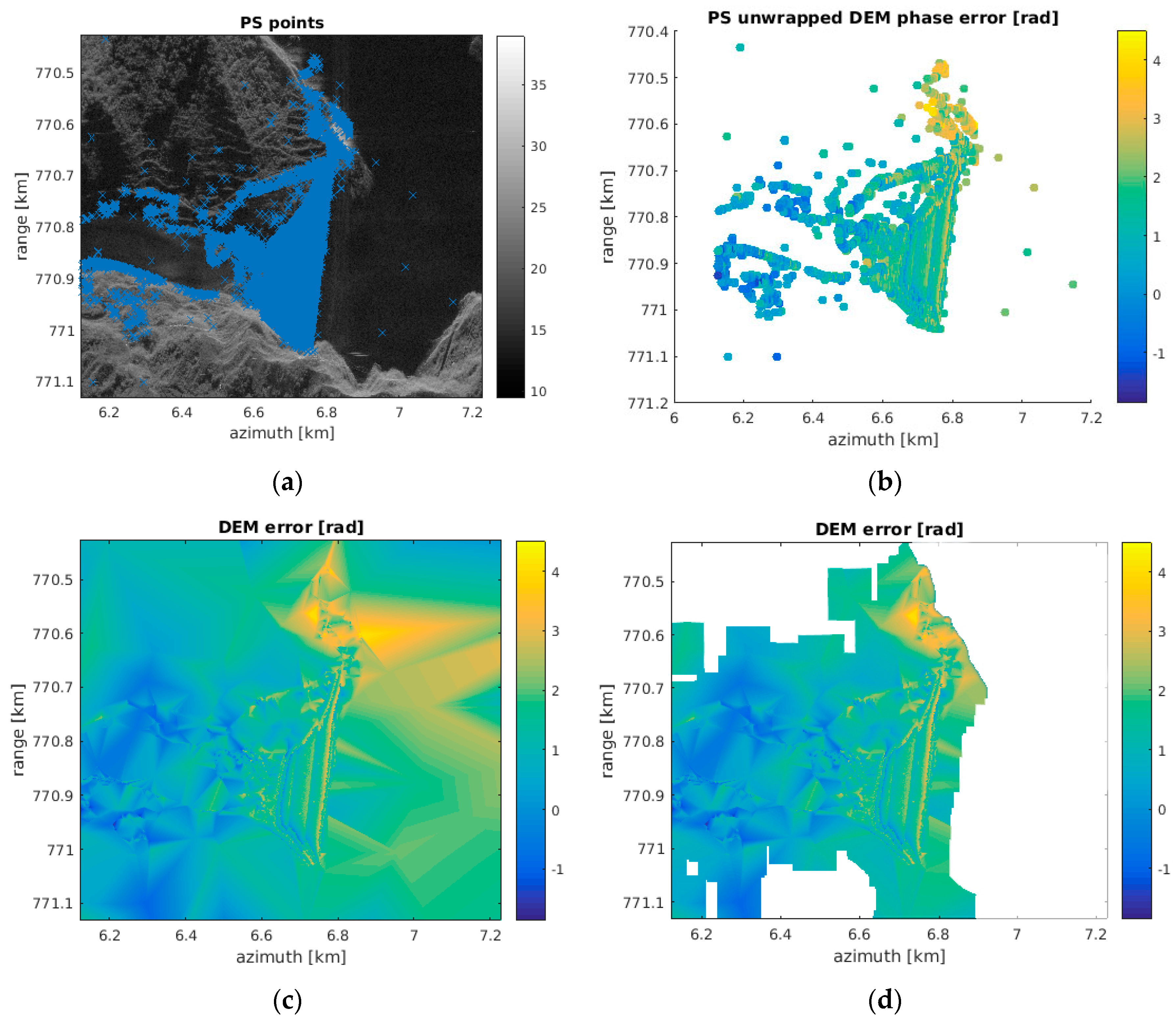
2.2. SAR Interferometry Phase (InSAR) Calibration with DEM Error

The phase calibration step is indispensable for TomoSAR imaging. In this paper, we employed the newly released TanDEM-X 12 m DEM available for very small geographical areas, alongside a new method to correct the phase via the SAR interferometric phase with the DEM error. The 12 m TanDEM-X DEM data were obtained through a data grant from DLR for 3D TomoSAR imaging over Zipingpu Dam, Dujiangyan, Sichuan Province, China, and its location is shown in Figure 3. A hill shaded map by GMT5 is shown in Figure 4.
DEM data, like all other spatial datasets, have errors (systematic and random errors as well as blunders). Therefore, it is critical to validate DEM products before using them for TomoSAR processing. The SRTM 30 m (absolute vertical accuracy ≤16 m) [31] and ICESAT GLA14 data (absolute vertical accuracy ≤1 m) [32] are used to assess the TanDEM-X 12 m DEM data. The vertical comparison accuracy (the height difference between the DEM and the ‘truth’ DEM) of the TanDEM-X 12 m DEM data in Dujiangyan can be summarized as follows: against the ICESat GLAS14 elevation data, the TanDEM-X 12 m DEM had an accuracy of 0.6 ± 16.1 m (mean ± standard deviation), and the RMSE was 16.1 m; against the SRTM 30 m data, the TanDEM-X 12 m DEM had an accuracy of −0.4 ± 15.9 m and the RMSE was 15.9 m. The standard deviation and RMSE of the difference between the 12 m TanDEM-X DEM data and SRTM data was a little bit larger; this might be because the 12 m TanDEM-X DEM data had errors, noise, and a lot of changes (e.g., new bridges, a new dam, earthquake deformation, landslide deformation, and so on in this area) after 2000 when the SRTM data were collected. The 12 m TanDEM-X DEM data had random errors (mainly from high frequency noise) that needed filtering before using them. As the TanDEM-X 12 m DEM included holes, the SRTM 30 m data were used to replace the holes within the Environment for Visualizing Images (ENVI). After that, the DEM data were edited using the noise removal and smoothing tool in ENVI. Then, the new improved TanDEM-X 12 m DEM was used for TomoSAR imaging.
In this study, a high-resolution DEM (e.g., the quality improved TanDEM-X 12 m DEM) was employed as the reference DEM in the co-registration step of TomoSAR processing. Then, SAR interferometry (InSAR) was applied. The interferograms between the slave image (10/08/2016) and the master image (25/07/2016) are shown in Figure 6 and Figure 7, which demonstrate the elimination of the DEM phase. The fringes could be clearly seen on the building, road, and dam areas in these figures, while the fringes were not clear in the mountain tree areas as the coherence was very low; this was caused by foreshortening, shadows, and the SAR layover in these complex mountain tree areas.
In addition, as the DEM simulation phase was used for deramping, the deramping phase in Equation (9) changed to that of Equation (14). As the simulation phase by DEM is based on an external DEM, and DEM data have errors, the DEM error phase φ D E M e r r o r must be taken into consideration in TomoSAR processing.
φ m = 4 π λ [ R R m ( 0 ) ] = φ s i m u _ m + φ D E M e r r o r ,
As is well-known, SLC complex data have errors, which include an atmospheric error (water vapor and ionosphere), orbit error, deformation (linear and nonlinear), and noise. The real complex data can be written as an ideal complex data plus all of the error phase φ e . φ e _ m a s t e r is the error phase of the master data and φ e _ s l a v e is the error phase of the slave data. In this way, the interferometric phase in Equation (14) becomes Equation (16). Based on Equations (8), (9), and (13), Equation (10) becomes Equation (17). In addition, the real flattening complex data are shown in Equation (15), then Equation (17) becomes Equation (18). It is known that φ I n S A R = φ D E M e r r o r + φ e _ m a s t e r φ e _ s l a v e is the interferometric phase after DEM flattening, as shown in Equation (19). This is because the InSAR phase is the DEM error phase, plus the master error phase, minus the slave error phase after flattening. Therefore, based on Equations (15) and (19), the TomoSAR processing Equation (18) becomes Equation (20). It can be seen from these equations that the InSAR phase can be used for phase calibration. With phase errors and the DEM error phase, Equation (20) should be used for the TomoSAR processing, as shown below. In Equation (20), I f l a t t e n i n g _ r e a l ( m ) is the flattening complex data using an external DEM, and φ I n S A R is the interferometric phase after flattening by this DEM. γ ( s ) in Equation (12) is the inversion results of TomoSAR processing along the s direction.   ξ m in Equation (4) is the spatial frequency, corresponding to the height s from the normal-slant-range direction ( s elevation direction).
I f l a t t e n i n g _ r e a l ( m ) = e x p ( j · φ s i m u _ m ) · Q ( m ) ,
φ m = 4 π λ [ R R m ( 0 ) ] = φ s i m u _ m + φ D E M e r r o r + φ e _ m a s t e r φ e _ s l a v e ,
p ( ξ m ) = e x p ( j ·   φ m ) ·   Q ( m ) = e x p ( j · φ s i m u _ m + j · φ D E M e r r o r + j · φ e m a s t e r j · φ e _ s l a v e ) ·   Q ( m ) = s m i n s m a x γ   ( s ) e x p ( j 2 π ξ m s ) d s ,
I f l a t t e n i n g _ r e a l ( m )   e x p ( j · φ D E M e r r o r + j · φ e m a s t e r j · φ e _ s l a v e   ) = p ( ξ m ) = s m i n s m a x γ   ( s ) e x p ( j 2 π ξ m s ) d s
φ I n S A R = φ D E M e r r o r + φ e _ m a s t e r φ e _ s l a v e ,
I f l a t t e n i n g _ r e a l ( m )   e x p ( j · φ I n S A R ) = p ( ξ m ) = s m i n s m a x γ   ( s ) e x p ( j 2 π ξ m s ) d s ,
After this phase calibration, the data are ready for super-resolution reconstruction via Capon and compressive sensing. However, the height reference is based on the strong scattering center after INSAR calibration. Hence, it is difficult to obtain a real height reference after this method. If geocoding is needed, control points are needed, or the result can be referenced to the DEM data after DEM error estimation and DEM error compensation based on Equation (23).
I f l a t t e n i n g _ r e a l ( m )   e x p ( j · φ I n S A R ) · e x p ( j · φ D E M e r r o r ) = s m i n s m a x γ ( s ) · e x p ( j · φ D E M e r r o r ) e x p ( j 2 π ξ m s ) d s ,
γ ( s ) = γ ( s ) · e x p ( j · φ D E M e r r o r ) ,
I f l a t t e n i n g _ r e a l ( m )   e x p ( j · ( φ I n S A R φ D E M e r r o r ) ) = s m i n s m a x γ ( s ) e x p ( j 2 π ξ m s ) d s ,
As shown in the above equations, φ I n S A R φ D E M e r r o r = φ e _ m a s t e r φ e s l a v e , and φ e _ m a s t e r φ e s l a v e represent the difference of phase errors, which includes an atmospheric error term (water vapor and ionosphere), orbit error, deformation (linear and nonlinear), and noise, hence why this step is called phase calibration.
Moreover, as shown in Equation (22) for all of the slave images, and in the right part of Equation (23), the DEM error phase e x p ( j · φ D E M e r r o r ) goes to γ   ( s ) and thus forms γ ( s ) , as shown in Equation (22) for all of the slave images. The DEM error phase does not influence the magnitude of γ   ( s ) , which means that the magnitude of γ   ( s ) is the same as the magnitude of γ ( s ) . The magnitude of γ ( s ) is the inversion results of TomoSAR processing. As a result, the InSAR with the DEM error phase method can be used for phase calibration. According to Equation (23), the accuracy of the DEM error estimation will influence the inversion results. After PS-InSAR (or SBAS InSAR), the DEM error can be obtained. Then, the DEM error of the whole image can be obtained by interpolation. Therefore, the DEM error was finally used to convert the unknown strong scattering center to the DEM data as the reference.

2.3. The Compressive Sensing Method

As SAR tomography is a semi-discrete problem ( γ ( s ) is continuous), it is necessary to discretise γ ( s ) for actual processing so that it can be converted into a discrete problem for solution. Let Δ s be the sampling interval of the NSR direction (elevation s) in the discretization process in the sampling interval [ S m i n ,   S m a x ] , then the total samples ( N ) are obtained. Next, the SAR tomography model can be written in the following form.
g Φ γ + e ,
where g is an M × 1 dimensional observation vector,
g = [ g ( ξ 1 ) , g ( ξ 2 ) , , g ( ξ M ) ] T ,
The ξ m is the spatial frequency corresponding to the height s in the NSR direction, Φ is a M × N dimensional matrix,
Φ = [ ϕ 1 , ϕ 2 , , ϕ M ] T ,
ϕ M = [ e x p ( j 2 π ξ m s 1 ) , e x p ( j 2 π ξ m s 2 ) , , e x p ( j 2 π ξ m s N ) ] T ,
γ is an N × 1 dimensional unknown signal vector, which is what we need to achieve at the end.
γ = [ γ ( s 1 ) , γ ( s 2 ) , , γ ( s N ) ] T ,
e is an M × 1 dimensional noise vector.
e = [ e ( ξ 1 ) e ( ξ 2 ) e ( ξ m ) ] T ,
According to the model in Equation (24), SAR tomography essentially reconstructs the unknown signal γ from the measured data g . Since the dimension of the measured data is much smaller than the dimension M < < N of the unknown signal γ , according to the classical signal reconstruction theory, a direct solution of Equation (24) is a pathological problem (cannot be solved in the classical signal reconstruction theory as the number of unknown parameters are larger than the number of the measurements). There are usually only a few strong scatterers in the same azimuth-distance resolution unit (one pixel), that is, γ is sparse in the height field. In practice, there is some unavoidable clutter in addition to the main strong scatterers, whose intensities are far less than those of strong scatterers [33,34,35]. Therefore, generally speaking, γ is compressible in the elevation region. In this case, the sparse basis is the Dirac basis, the sparse basis matrix Ψ   =   I , I is the N × N dimension unit matrix, γ   =   Ψ   γ   =   γ . In view of this, we can solve the problem of SAR tomography in the theoretical framework of compressive sensing. The result is
m i n γ γ 1   subject   to   g   = Φ γ ,
For a given K , since γ is compressible in the elevation region, that is, the sparse basis matrix Ψ   =   I , γ   =   Ψ ,   γ   =   γ , quadratic relaxation can provide a good approximation of the sparsest solution. When noise is considered, Equation (30) becomes
M = O ( K   l o g   N ) ,
m i n γ γ 1   subject   to   g Φ γ σ e   ,
where M is the smallest number of SLC data for CS method; σ e is the standard deviation of the noise. If K is not known and measurement noise exists, Equation (30) can be approximated by:
γ ^ = arg m i n γ ( | | g Φ γ | | 2 2 + λ k | | γ | | 1 ) ,
where γ ^ = arg m i n γ ( ) means the optimum estimate of γ ; γ ^ is the best optimum estimate of γ , when | | g Φ γ | | 2 2 + λ k | | γ | | 1 is the smallest and γ γ ^ ; λ k is a Lagrange multiplier depending on the number of samples N [36] and the noise level σ e . Equation (33) consists of an L2 norm residual and an L1 norm regularizer and Equation (33) can be interpreted as a Bayesian estimate with an exponential prior favoring sparse solution. By scaling down via the L1 and L2 norm minimization method, model selection, parameter estimation, and least-squares estimation, all the results can be achieved.

3. Results

3.1. Test Sites and COSMO-SkyMed Spaceborne SAR

The densely vegetated mountainous rural areas at Zipingpu Dam, Dujiangyan, Sichuan, China were employed as a test area, as shown in Figure 8a,b. Figure 8c displays a small test subarea over the Zipingpu Dam for TomoSAR imaging. In 3D SAR imaging (SAR tomography), 14 COSMO-SkyMed Spotlight ascending data stacks are used, as shown in Table 1. Figure 8 reveals the TDX-DEM 12 m and SRTM 30 m data as well as the orbit information. In this test, the reference terrain-TanDEM-X 12 m data (Figure 8d) were used for deramping with all of the TomoSAR height results being based on the TanDEM-X DEM12 m surface. Work on the dam was started on 29/03/2001 and completed on 30/09/2005. However, the SRTM data were acquired in February 2000. Therefore, Figure 8f demonstrates the height difference and shape of the dam. Moreover, after PS-InSAR, the DEM errors of each PS point are estimated. Then, the DEM error of the whole image can be obtained by interpolation. The DEM error map of 03/06/2016 via PS-InSAR is shown in Figure 9. After estimating the DEM errors, the phase of this DEM error will be compensated via simple phase addition and subtraction for TomoSAR processing based on Equation (23).

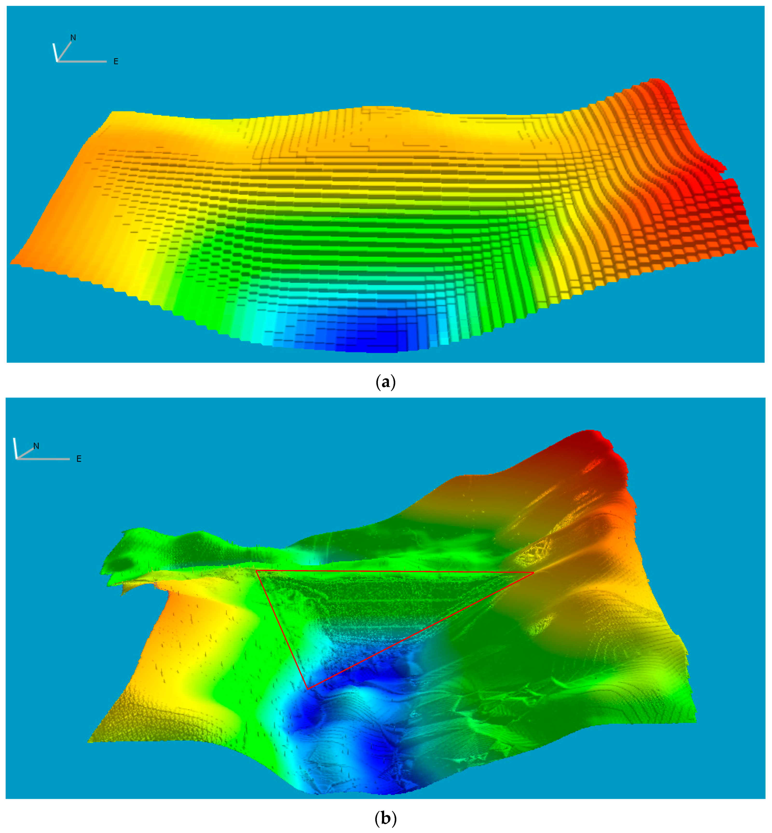
3.2. TomoSAR Results and Fieldwork for Validation

The results derived from the compressive sensing [33] method in the sub-test area after InSAR phase calibration and DEM referenced correction is shown in Figure 10. All results were referenced to the DEM elevation, which can be applied for geocoding using SAR observation geometry. After CS imaging, the errors were filtered, and targets selected by the improved constant false alarm rate (CFAR) method for our application. First, the mean value and standard deviation were calculated, and all peaks were found along the height direction; then, when the amplitude of the peaks was larger than three times the standard deviation plus the mean value, they were selected as targets. Moreover, the results illustrated a strong backscatter curve line with the few targets around it, confirming that the X band data could hardly penetrate trees. The simulation using the COSMO-SkyMed X-band satellite parameters with the baseline distribution of the dataset used demonstrated that the theoretical vertical precision of the extraction elevation was 0 m.
Finally, after geocoding (adding the TanDEM-X 12 m DEM height), the 1 m TomoSAR elevation extraction results of the X-band COSMO-SkyMed Spotlight data can be obtained, as shown in Figure 10. Compared to the TanDEM-X 12 m DEM data in Figure 10a, the results of the 1 m TomoSAR in Figure 10b exhibited better resolution. As shown in Figure 10b, there are two line steps on the dam in the 1 m TomoSAR imaging results, which can also be observed in the Lidar and photos in Figure 11a–c.
As the X band has little vegetation penetration capability and no penetration for the X band at all for the man-made dam, only one point of the TomoSAR imaging result for each SAR pixel along the height direction in the dam area could be validated using Lidar data. Furthermore, as the TomoSAR results were referenced to the TANDEM-X 12 m data, the results already have a set of absolute coordinates after geocoding (adding DEM height). If the high accuracy of the position is needed, the Lidar or other control data can be used as control points for geocoding.
Fieldwork to acquire terrestrial Lidar data and photos were collected at Zipingpu Dam, Dujiangyan, China between 24/09/2017 and 29/09/2017. The photos of the Zipingpu dam are shown in Figure 11a,b. The Lidar data collected by the ground-based V-Line 3D Terrestrial Laser Scanner (TLS) RIEGL VZ-1000 at Zipingpu Dam were used for validation, as shown in Figure 11c.
Finally, and Figure 12 and Table 2 indicate the absolute difference map between the X-band TomoSAR imaging result and the Lidar data over the field site at Dujiangyan and the height difference statistical results. The map shows that the compressive sensing result had a good match with Lidar data after geocoding. As shown in Table 2, the maximum difference was 8.6 m, the minimum difference was −8.5 m, the mean difference was 0.11 m, the standard deviation was 2.81 m, and the RMSE was 2.82 m. After masking out the tree and mountain areas, the maximum difference of the dam area was 5.3 m, the minimum difference was −5.7 m, the mean difference was 0.25 m, the standard deviation was 1.04 m, and the RMSE was 1.07 m (over the dam area). These results demonstrate that the compressive sensing result showed a good match with the Lidar data after geocoding. Therefore, the TomoSAR imaging algorithm appears to work satisfactorily and result in a 1 m DEM. These high resolution TomoSAR results in the dam area are outstanding for application because they match very well with the Lidar data and have high accuracy.
Finally, we show several azimuth lines along the range direction (points of each line are stored in Google Earth KML format, the red colour points in the picture) of our TomoSAR results in Google Earth, shown in Figure 13 below.

4. Discussion

First, all of the SAR SLC data were co-registered in the radar coordinate system to sub-pixel accuracy for TomoSAR processing. This was based on the master image orbit information and external DEM. Thereafter, a precise orbit was used to estimate the orbit baseline. Moreover, because DEM deramping establishes the spectrum relationship (based on the perpendicular baseline) between the observed SAR images and 3D SAR tomographic reconstruction inversion parameters, 3D SAR inversion is possible. The reference slant range used in the deramping process can be the central range of each image using the radar transmission time delay and velocity, or the distance between the radar antenna phase center of each image and a reference terrain (e.g., external DEM data). It should be noted that the only differences between the two methods are the zero-point benchmark and phase errors. According to our experiment, the coarse DEM (TanDEM-X 12 m) was used for deramping without additional atmospheric phase errors in the accurate reference slant range calculation. However, even after pre-processing of the high resolution DEM, the DEM still had elevation errors, which may also have an impact on the TomoSAR results. Therefore, the phase calibration step is indispensable for TomoSAR imaging, eventually ensuring the accuracy of the inversion results. After PS-InSAR (or SBAS InSAR), the DEM error was estimated and obtained. Then, the phase calibration method based on SAR interferometry (InSAR) and DEM error estimation and compensation for 3D TomoSAR imaging was used. Based on this method, the accuracy of the DEM error estimation will affect the inversion results. However, the high accuracy of the DEM error estimation in a constructed facility area can guarantee good performance for the phase calibration.
In the Dujiangyan test area, it was difficult to obtain favorable compressive sensing results using the original baseline, while compressive sensing worked successfully after using the improved baseline with the new phase calibration. The compressive sensing results in the dam area had a good match with the Lidar data. Although there were some differences except for the 0 m difference, they were around 0.18 m difference on average, which might be caused by other errors such as DEM uncertainty, orbital, tropospheric and ionospheric phase distortion, and thermal noise.
The CS algorithm is generally executed using SLC data (without averaging for noise filtering), which is automatically performed in the stack dimension using the SAR model and sparsity driven estimation technique to characterize a minimal number (<4) of targets in the measured signal. Therefore, CS is well-adapted to discrete scatterers or targets as well as 3D and 4D high resolution tomographic reconstruction. The results demonstrate that the X band had little penetration capability, and thus cannot be used for forest structure reconstruction. However, it can be used to extract the canopy top, the shape of the constructed structures (dam, buildings, and manufactured facilities), and the top of the 3D terrain, which is optimal for high resolution DSM extraction and target detection.

5. Conclusions

In this paper, based on our theoretical study and mathematical derivation, a systematic TomoSAR algorithm and the methods were described, demonstrated, tested, and analyzed to achieve 3D tomographic SAR imaging results using COSMO-SkyMed X band data over Zipinpu Dam, Dujiangyan, Sichuan, China. We demonstrated that in 3D SAR tomography, phase calibration plays a crucial role in the data processing. With the newly released TanDEM-X 12 m DEM and suitable pre-processing, this study proposes a new phase calibration method based on SAR interferometry (InSAR) and DEM error estimation and compensation for 3D TomoSAR imaging. Then, the super-resolution reconstruction CS method was studied, which demonstrated that the X band data with the CS method are not suitable for forest structure reconstruction, but fit for the reconstruction of manufactured facilities (dam) and buildings in the urban area. Finally, the fieldwork and validation were described, and the results revealed that our methods worked properly using COSMO-SkyMed X band data at Zipinpu Dam, Dujiangyan, Sichuan, China.

Author Contributions

Conceptualization, L.F. and J.-P.M.; Methodology, L.F.; Validation, L.F., C.D., C.Y. and J.Z.; Writing—original draft preparation, L.F.; Writing—review and editing, C.D., C.Y., J.Z. and J.-P.M.; Supervision, J.-P.M. and J.Z.; Project administration, J.-P.M.; Funding acquisition, J.-P.M., C.D. and C.Y. All authors have read and agreed to the published version of the manuscript.

Funding

This research was funded by CSC and the UCL MAPS Dean prize through a PhD studentship at UCL-MSSL.

Data Availability Statement

Not applicable.

Acknowledgments

Many thanks to CSC and the UCL MAPS Dean prize for a PhD studentship at UCL-MSSL. Many thanks to DLR for the TanDEM-X data grant of 12 m DEM under grant number DEM_METH1620 as well as Space Catapult, Harwell space campus and Terri Freemantle, in particular, for arranging the provision of the CORSAIR011 data. Many thanks to Tengfei Xue, Qisong Jiao, and Hongbo Jiang (China Earthquake Administration) for the fieldwork and data processing. Many thanks to Stefano Tebaldini (Politecnico di Milano) and Laurent Ferro-Famil (University of Rennes) for the data and code, and the ESA for the data and organizing the ESA 4th advanced course on radar polarimetry. Many thanks to the COMET community for organizing the COMET InSAR Training Workshop 2017. Many thanks to David Bekaert from JPL to provide the InSAR code for research. Many thanks to Shaun Quegan from the University of Sheffield and Tim Wright from the University of Leeds for their comments.

Conflicts of Interest

The authors declare no conflict of interest.

References

  1. Reigber, A.; Moreira, A. First demonstration of airborne SAR tomography using multibaseline L-band data. IEEE Trans. Geosci. Remote Sens. 2000, 38, 2142–2152. [Google Scholar] [CrossRef]
  2. Fornaro, G.; Serafino, F.; Soldovieri, F. Three-dimensional focusing with multipass SAR data. IEEE Trans. Geosci. Remote Sens. 2003, 41, 507–517. [Google Scholar] [CrossRef]
  3. Nannini, M.; Scheiber, R.; Horn, R. Imaging of targets beneath foliage with SAR tomography. In Proceedings of the EUSAR 2008: 7th European Conference on Synthetic Aperture Radar, Friedrichshafen, Germany, 2–5 June 2008; pp. 1–4. [Google Scholar]
  4. Lombardini, F.; Cai, F.; Pasculli, D. Spaceborne 3-D SAR tomography for analyzing garbled urban scenarios: Single-look superresolution advances and experiments. IEEE J. Sel. Top. Appl. Earth Obs. Remote Sens. 2013, 6, 960–968. [Google Scholar] [CrossRef]
  5. Lombardini, F.; Cai, F. Evolutions of Diff-Tomo for Sensing Subcanopy Deformations and Height-Varying Temporal Coherence. In Proceedings of the Fringe 2011, Frascati, Italy, 19–23 September 2011; p. 43. [Google Scholar]
  6. Lombardini, F. Differential tomography: A new framework for SAR interferometry. IEEE Trans. Geosci. Remote Sens. 2005, 43, 37–44. [Google Scholar] [CrossRef]
  7. Lombardini, F.; Pardini, M. Superresolution differential tomography: Experiments on identification of multiple scatterers in spaceborne SAR data. IEEE Trans. Geosci. Remote Sens. 2012, 50, 1117–1129. [Google Scholar] [CrossRef]
  8. Lombardini, F.; Viviani, F.; Cai, F.; Dini, F. Forest Temporal Decorrelation: 3D Analyses and Processing in the Diff-Tomo Framework. In Proceedings of the Geoscience and Remote Sensing Symposium (IGARSS), 2013 IEEE International, Melbourne, Australia, 21–26 July 2013; pp. 1202–1205. [Google Scholar]
  9. Tebaldini, S.; Rocca, F. Multibaseline polarimetric SAR tomography of a boreal forest at P-and L-bands. IEEE Trans. Geosci. Remote Sens. 2012, 50, 232–246. [Google Scholar] [CrossRef]
  10. Piau, P. Performances of the 3D-SAR Imagery. In Proceedings of the IGARSS ’94—1994 IEEE International Geoscience and Remote Sensing Symposium, Pasadena, CA, USA, 8–12 August 1994; pp. 2267–2271. [Google Scholar]
  11. Jakowatz, C.V.; Thompson, P. A new look at spotlight mode synthetic aperture radar as tomography: Imaging 3-D targets. IEEE Trans. Image Process. 1995, 4, 699–703. [Google Scholar] [CrossRef] [PubMed]
  12. Homer, J.; Longstaff, I.; She, Z.; Gray, D. High resolution 3-D imaging via multi-pass SAR. IEEE Proc.-Radar Sonar Navig. 2002, 149, 45–50. [Google Scholar] [CrossRef] [Green Version]
  13. Pasquali, P.; Prati, C.; Rocca, F.; Seymour, M.; Fortuny, J.; Ohlmer, E.; Sieber, A. A 3-D Sar Experiment with EMSL Data. In Proceedings of the 1995 International Geoscience and Remote Sensing Symposium, IGARSS 95. Quantitative Remote Sensing for Science and Applications, Firenze, Italy, 10–14 July 1995; pp. 784–786. [Google Scholar]
  14. Zhu, X.X.; Bamler, R. Very high resolution spaceborne SAR tomography in urban environment. IEEE Trans. Geosci. Remote Sens. 2010, 48, 4296–4308. [Google Scholar] [CrossRef] [Green Version]
  15. Zhu, X.X.; Bamler, R. Tomographic SAR inversion by L1 norm regularization—The compressive sensing approach. IEEE Trans. Geosci. Remote Sens. 2010, 48, 3839–3846. [Google Scholar] [CrossRef] [Green Version]
  16. Xiang, Z.X.; Bamler, R. Compressive Sensing for High Resolution Differential SAR Tomography-the SL1MMER algorithm. In Proceedings of the Geoscience and Remote Sensing Symposium (IGARSS), 2010 IEEE International, Honolulu, HI, USA, 25–30 July 2010; pp. 17–20. [Google Scholar]
  17. Fornaro, G.; Reale, D.; Serafino, F. Four-dimensional SAR imaging for height estimation and monitoring of single and double scatterers. Geosci. Remote Sens. IEEE Trans. 2009, 47, 224–237. [Google Scholar] [CrossRef]
  18. Huang, Y.; Ferro-Famil, L.; Reigber, A. Under-foliage object imaging using SAR tomography and polarimetric spectral estimators. IEEE Trans. Geosci. Remote Sens. 2012, 50, 2213–2225. [Google Scholar] [CrossRef] [Green Version]
  19. Huang, Y.; Ferro-Famil, L.; Reigber, A. Under-foliage target detection using multi-baseline L-band PolInSAR data. In Proceedings of the 2013 14th International Radar Symposium (IRS), Dresden, Germany, 19–21 June 2013; pp. 449–454. [Google Scholar]
  20. Zhu, X.X.; Bamler, R. Tomographic SAR inversion from mixed repeat- and single-Pass data stacks—The TerraSAR-X/TanDEM-X case. In Proceedings of the XXII ISPRS Congress, Melbourne, Australia, 25 August–1 September 2012. [Google Scholar]
  21. Ferro-Famil, L.; Leconte, C.; Boutet, F.; Phan, X.-V.; Gay, M.; Durand, Y. PoSAR: A VHR tomographic GB-SAR system application to snow cover 3-D imaging at X and Ku bands. In Proceedings of the 2012 9th European Radar Conference, Amsterdam, The Netherlands, 31 October–2 November 2012; pp. 130–133. [Google Scholar]
  22. Lombardini, F.; Cai, F. 3D tomographic and differential tomographic response to partially coherent scenes. In Proceedings of the IGARSS 2008—2008 IEEE International Geoscience and Remote Sensing Symposium, Boston, MA, USA, 6–11 July 2008. [Google Scholar]
  23. Pardini, M.; Papathanassiou, K. Robust Estimation of the Vertical Structure of Forest with Coherence Tomography. In Proceedings of the ESA POLinSAR Workshop, Frascati, Italy, 24–28 January 2011. [Google Scholar]
  24. Fornaro, G.; Lombardini, F.; Serafino, F. Three-dimensional multipass SAR focusing: Experiments with long-term spaceborne data. IEEE Trans. Geosci. Remote Sens. 2005, 43, 702–714. [Google Scholar] [CrossRef]
  25. Siddique, M.A.; Hajnsek, I.; Wegmüller, U.; Frey, O. Towards the integration of SAR tomography and PSI for improved deformation assessment in urban areas. In Proceedings of the FRINGE Workshop, Frascati, Italy, 23–27 March 2015. [Google Scholar]
  26. Fornaro, G.; Serafino, F. Spaceborne 3D SAR Tomography: Experiments with ERS data. In Proceedings of the IGARSS 2004. 2004 IEEE International Geoscience and Remote Sensing Symposium, Anchorage, AK, USA, 20–24 September 2004; pp. 1240–1243. [Google Scholar]
  27. Eineder, M. Efficient simulation of SAR interferograms of large areas and of rugged terrain. IEEE Trans. Geosci. Remote Sens. 2003, 41, 1415–1427. [Google Scholar] [CrossRef] [Green Version]
  28. Lu, Z.; Dzurisin, D. InSAR imaging of Aleutian volcanoes. In InSAR Imaging of Aleutian Volcanoes; Springer: New York, NY, USA, 2014; pp. 87–345. [Google Scholar]
  29. Parker, A.L. InSAR Observations of Ground Deformation: Application to the Cascades Volcanic Arc; Springer: New York, NY, USA, 2016. [Google Scholar]
  30. Ketelaar, V. Satellite Radar Interferometry, Remote Sensing and Digital Image Processing; Springer: Dordrecht, The Netherlands, 2009. [Google Scholar]
  31. Rodriguez, E.; Morris, C.S.; Belz, J.E. A global assessment of the SRTM performance. Photogramm. Eng. Remote Sens. 2006, 72, 249–260. [Google Scholar] [CrossRef] [Green Version]
  32. Feng, L.; Muller, J.-P. ICESAT Validation of TANDEM-X I-DEMs over the UK. Int. Arch. Photogramm. Remote Sens. Spat. Inf. Sci. 2016, XLI–B4, 129–136. [Google Scholar] [CrossRef] [Green Version]
  33. Zhu, X. Very High Resolution Tomographic SAR Inversion for Urban Infrastructure Monitoring—A Sparse and Nonlinear Tour. Ph.D. Thesis, Technische Universität München, München, Germany, 2011. [Google Scholar]
  34. Candes, E.J.; Wakin, M.B.; Boyd, S.P. Enhancing sparsity by reweighted ℓ 1 minimization. J. Fourier Anal. Appl. 2008, 14, 877–905. [Google Scholar] [CrossRef]
  35. Xilong, S.; Anxi, Y.; Zhen, D.; Diannong, L. Three-dimensional SAR focusing via compressive sensing: The case study of angel stadium. IEEE Geosci. Remote Sens. Lett. 2012, 9, 759–763. [Google Scholar] [CrossRef]
  36. Chen, S.S.; Donoho, D.L.; Saunders, M.A. Atomic decomposition by basis pursuit. SIAM Rev. 2001, 43, 129–159. [Google Scholar] [CrossRef] [Green Version]
Figure 1. A schematic of the TomoSAR imaging geometry. The elevation synthetic aperture was built up by multi-pass SAR data from slightly different view angles. The flight direction was orthogonal out of the plane. Δb is the elevation synthetic aperture length, x is the azimuth direction, r is the range direction, and s is the elevation direction.
Remotesensing 14 04093 g001
Figure 2. The workflow of the 3D tomographic SAR imaging, APS refers to the atmospheric phase screen, phase error compensation refers to the SAR interferometry phase with the DEM error phase calibration in this study.
Remotesensing 14 04093 g002
Figure 3. The location of the 12 m TanDEM-X DEM data, the red box area is the Dujiangyan TomoSAR test area, the two green boxes are the two 12 m TanDEM-X DEM tiles (1 degree × 1 degree for a tile) of the 12 m DEM map of the two tiles shown in Figure 5, and the background image is a Google Earth image (image source: Landsat image/Copernicus).
Remotesensing 14 04093 g003
Figure 4. The TanDEM-X 12 m DEM colorized and hill-shaded map of the two 12 m TanDEM-X DEM tiles whose location is shown in Figure 3; the red rectangle box area is the study site; the blue areas are holes caused by low coherence or shadow.
Remotesensing 14 04093 g004
Figure 5. The quality improvement editing of the TanDEM-X 12 m DEM data (a) after hole replacement using the SRTM-V3 30 m data; (b) after hole replacement, noise removal, and smooth filtering, the line features are clearer within the red box.
Remotesensing 14 04093 g005
Figure 6. The interferogram between 10/08/2016 and master 25/07/2016 SLC after flattening and filtering in the radar coordinate system, the base map is the amplitude of the interferogram complex data; the phase is superimposed on the base map. The fringes can be clearly seen on the bridge, buildings (top−right), road, and dam areas in the figure. The fringes of the dam area in the red rectangle box can be seen in Figure 7 more clearly after flattening and filtering in the radar coordinate system. The fringes over the dam areas are displayed in more detail in Figure 7 below.
Remotesensing 14 04093 g006
Figure 7. A zoom−in map of the interferogram (the red rectangle box area shown in Figure 6) between the slave 20,160,810 SLC and master 20,160,725 SLC; the fringes can be observed over the dam area. (a) The interferogram phase after flattening and filtering was laid out on the amplitude of the interferogram complex data. (b) The interferogram phase after flattening and filtering in the same area.
Remotesensing 14 04093 g007
Figure 8. The test site and a small test subarea at Zipingpu Dam in Dujiangyan, Sichuan, China (master image is 25/07/2016). (a) The test site in Sichuan China, the red area is COSMO-SkyMed Spotlight data stacks, the background image is a Google Earth image (image source: Landsat image/Copernicus). (b) Overview of Zipingpu Dam (Source: Tianditu, China). (c) SAR image of the test subarea, the color of the figure is the average amplitude of all SAR SLC stacks, the unit is dB. (d) Azimuth test line on TanDEM. (e) Azimuth test line on the SRTM 30 m data. (f) The azimuth test line of the height difference between the TanDEM-X DEM 12 m DEM and SRTM 30 m DEM.
Remotesensing 14 04093 g008aRemotesensing 14 04093 g008b
Figure 9. The DEM error maps in the dam area. (a) The PS points via PS−InSAR in the test area (03/06/2016). (b) The unwrapped phase of DEM error map at the PS points (03/06/2016), PS points over the surface of the water might be caused by range or azimuth ambiguities. (c) The unwrapped phase of the DEM error map via PS−InSAR (03/06/2016). (d) The unwrapped phase of the DEM error map via PS−InSAR (03/06/2016); the river and no PS point in the 100 m range are masked.
Remotesensing 14 04093 g009
Figure 10. The TomoSAR results of the sub-test area at Zipingpu Dam of the Dujiangyan test area in China. (a) The TanDEM-X 12 m DEM at Dujiangyan. (b) The TomoSAR 1 m resolution imaging result of the COSMO-SkyMed Spotlight data at Dujiangyan, where the elevation extraction appears successful when compared to (a). The values retrieved over the areas covered by water were not reliable, which were not used for validation. The red triangle area is the validation area, in which the Lidar data were obtained in the fieldwork.
Remotesensing 14 04093 g010
Figure 11. The fieldwork at Zipingpu Dam in Dujiangyan, Sichuan, China, LIDAR point cloud of Zipingpu Dam for validation obtained via a RIEGL VZ-1000. (a) Zipingpu Dam in Dujiangyan; (b) Zipingpu Dam in Dujiangyan; (c) Lidar point cloud of Zipingpu Dam, only the dam data were obtained in the fieldwork (the red triangle area shown in Figure 10).
Remotesensing 14 04093 g011
Figure 12. The difference map between the X-band TomoSAR imaging result and the LIDAR data of the fieldwork at Zipingpu Dam; the difference is the absolute value (absolute distance) of the difference.
Remotesensing 14 04093 g012
Figure 13. The TomoSAR results displayed in Google Earth, where the TomoSAR results of six azimuth lines in the test area were input into Google Earth for viewing.
Remotesensing 14 04093 g013
Table 1. The ascending COSMO-SkyMed Spotlight data stacks, the master image is 25/07/2016.
IDIncidence AngleTimeTrack TypeBaseline (m)
137.6603/06/2016Ascending−373.44
237.6611/06/2016Ascending−289.25
337.6619/06/2016Ascending743.28
437.6623/06/2016Ascending920.38
537.6605/07/2016Ascending−431.28
637.6609/07/2016Ascending−629.15
737.6625/07/2016Ascending0
837.6606/08/2016Ascending820.31
937.6610/08/2016Ascending203.46
1037.6622/08/2016Ascending−435.71
1137.6626/08/2016Ascending−140.25
1237.6607/09/2016Ascending186.17
1337.6611/09/2016Ascending611.54
1437.6623/09/2016Ascending−330.33
Table 2. The results of the validation statistics.
Basic StatsAreaMin (m)Max (m)Mean (m)Stdev σ (m)RMSE (m)
TomoSAR-LidarDam and mountain trees−8.58.60.112.812.82
TomoSAR-LidarDam−5.75.30.251.041.07
Publisher’s Note: MDPI stays neutral with regard to jurisdictional claims in published maps and institutional affiliations.

