
Integration of Photogrammetric and Spectral Techniques for Advanced Drone-Based Bathymetry Retrieval Using a Deep Learning Approach

 , , , and
Abstract
:
1. Introduction
1.1. Optical Remote Sensing in Seafloor Mapping
1.2. Satellite-Derived Bathymetry
1.3. Structure from Motion
1.4. Aim of the Study
2. Methodology
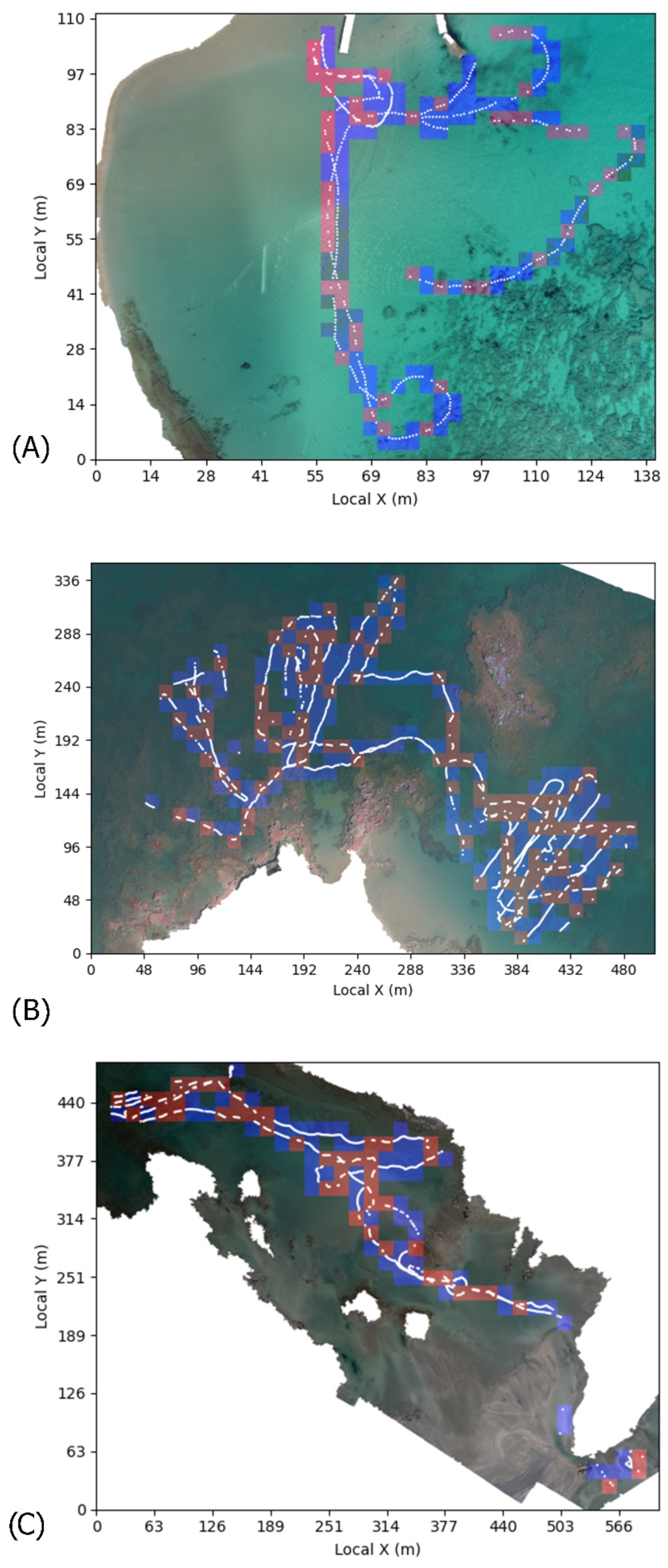
2.1. Study Areas
2.2. Onshore Survey and Drone Platform Configuration
2.3. USV Surveys
2.4. Structure from Motion
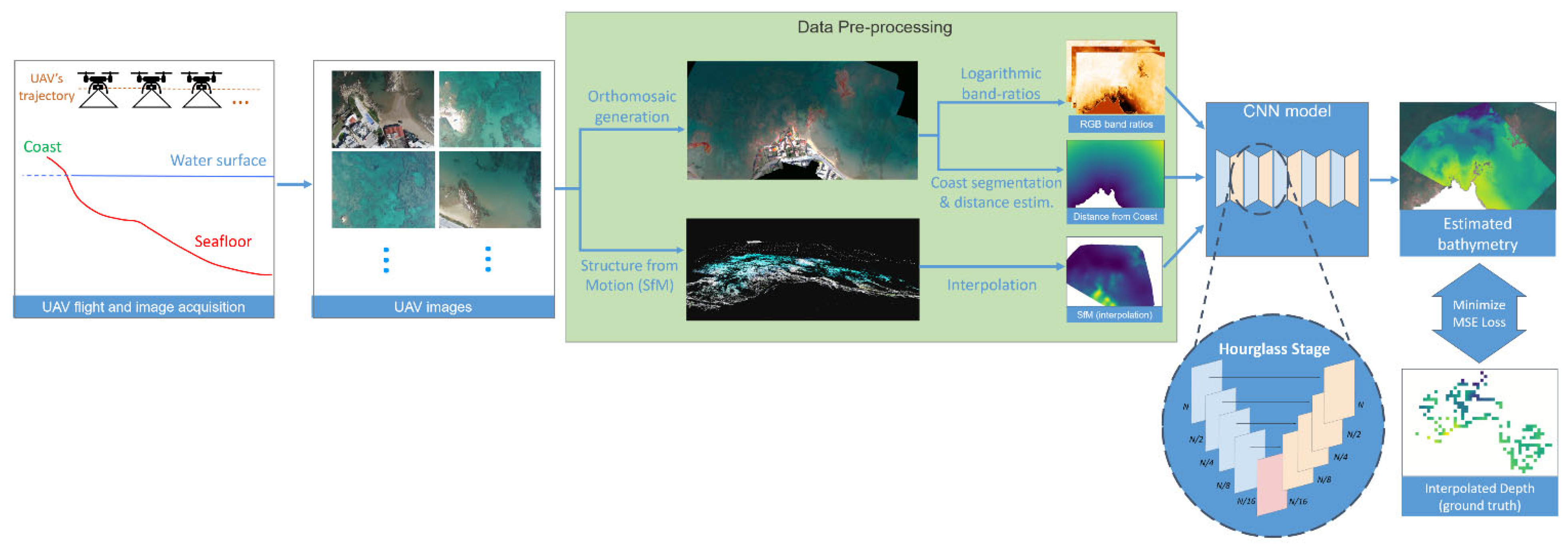
2.5. Data Pre-Processing
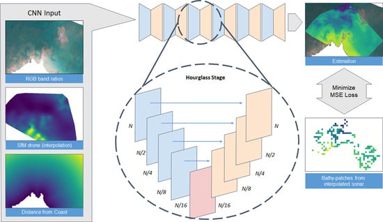
2.6. Convolutional Network Architecture and Training Set
3. Results
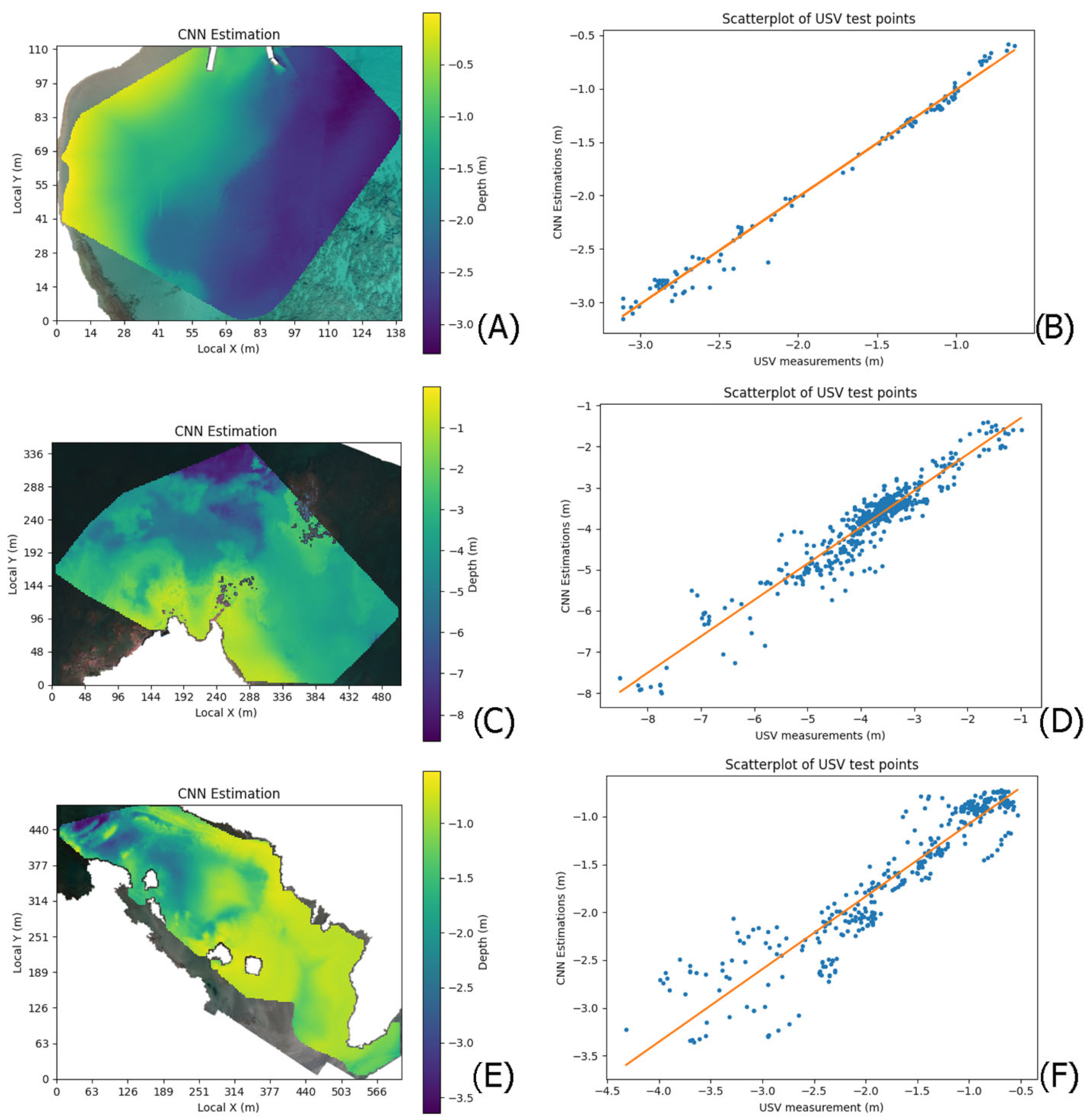
3.1. Bathymetry Results on the Study Areas
3.2. Ablation Study
3.3. Sensitivity Analysis of the Train–Test Split
3.4. Comparison with Artificial Neural Networks and Conventional Machine Learning Methods
3.5. Cross-Validation Study
4. Discussion
4.1. Algorithm Performance
4.2. Future Considerations
5. Conclusions
Author Contributions
Funding
Data Availability Statement
Acknowledgments
Conflicts of Interest
References
- Davidson, M.; Van Koningsveld, M.; de Kruif, A.; Rawson, J.; Holman, R.; Lamberti, A.; Medina, R.; Kroon, A.; Aarninkhof, S. The CoastView Project: Developing Video-Derived Coastal State Indicators in Support of Coastal Zone Management. Coast. Eng. 2007, 54, 463–475. [Google Scholar] [CrossRef]
- de Swart, H.E.; Zimmerman, J.T.F. Morphodynamics of Tidal Inlet Systems. Annu. Rev. Fluid Mech. 2009, 41, 203–229. [Google Scholar] [CrossRef]
- van Dongeren, A.; Plant, N.; Cohen, A.; Roelvink, D.; Haller, M.C.; Catalán, P. Beach Wizard: Nearshore Bathymetry Estimation through Assimilation of Model Computations and Remote Observations. Coast. Eng. 2008, 55, 1016–1027. [Google Scholar] [CrossRef]
- Janowski, L.; Wroblewski, R.; Rucinska, M.; Kubowicz-Grajewska, A.; Tysiac, P. Automatic Classification and Mapping of the Seabed Using Airborne LiDAR Bathymetry. Eng. Geol. 2022, 301, 106615. [Google Scholar] [CrossRef]
- Garcia, R.A.; Lee, Z.; Hochberg, E.J. Hyperspectral Shallow-Water Remote Sensing with an Enhanced Benthic Classifier. Remote Sens. 2018, 10, 147. [Google Scholar] [CrossRef]
- Kobryn, H.T.; Wouters, K.; Beckley, L.E.; Heege, T. Ningaloo Reef: Shallow Marine Habitats Mapped Using a Hyperspectral Sensor. PLoS ONE 2013, 8, e70105. [Google Scholar] [CrossRef]
- Purkis, S.J.; Gleason, A.C.R.; Purkis, C.R.; Dempsey, A.C.; Renaud, P.G.; Faisal, M.; Saul, S.; Kerr, J.M. High-Resolution Habitat and Bathymetry Maps for 65,000 Sq. Km of Earth’s Remotest Coral Reefs. Coral Reefs 2019, 38, 467–488. [Google Scholar] [CrossRef]
- Carvalho, R.C.; Hamylton, S.; Woodroffe, C.D. Filling the ‘White Ribbon’ in Temperate Australia: A Multi-Approach Method to Map the Terrestrial-Marine Interface. In Proceedings of the 2017 IEEE/OES Acoustics in Underwater Geosciences Symposium (RIO Acoustics), Rio de Janeiro, Brazil, 25–27 July 2017; pp. 1–5. [Google Scholar]
- Kenny, A.J.; Cato, I.; Desprez, M.; Fader, G.; Schüttenhelm, R.T.E.; Side, J. An Overview of Seabed-Mapping Technologies in the Context of Marine Habitat Classification. ICES J. Mar. Sci. 2003, 60, 411–418. [Google Scholar] [CrossRef]
- Costa, B.M.; Battista, T.A.; Pittman, S.J. Comparative Evaluation of Airborne LiDAR and Ship-Based Multibeam SoNAR Bathymetry and Intensity for Mapping Coral Reef Ecosystems. Remote Sens. Environ. 2009, 113, 1082–1100. [Google Scholar] [CrossRef]
- Taramelli, A.; Cappucci, S.; Valentini, E.; Rossi, L.; Lisi, I. Nearshore Sandbar Classification of Sabaudia (Italy) with LiDAR Data: The FHyL Approach. Remote Sens. 2020, 12, 1053. [Google Scholar] [CrossRef] [Green Version]
- Brock, J.C.; Purkis, S.J. The Emerging Role of Lidar Remote Sensing in Coastal Research and Resource Management. J. Coast. Res. 2009, 10053, 1–5. [Google Scholar] [CrossRef]
- Klemas, V. Beach Profiling and LIDAR Bathymetry: An Overview with Case Studies. J. Coast. Res. 2011, 277, 1019–1028. [Google Scholar] [CrossRef]
- Freire, R.; Pe’eri, S.; Madore, B.; Rzhanov, Y.; Alexander, L.; Parrish, C.; Lippmann, T. Monitoring Near-Shore Bathymetry Using a Multi-Image Satellite-Derived Bathymetry Approach; International Hydrographic Organization: National Harbor, MD, USA, 2015. [Google Scholar]
- Albert, A.; Mobley, C.D. An Analytical Model for Subsurface Irradiance and Remote Sensing Reflectance in Deep and Shallow Case-2 Waters. Opt. Express 2003, 11, 2873–2890. [Google Scholar] [CrossRef]
- Lee, Z.; Carder, K.L.; Mobley, C.D.; Steward, R.G.; Patch, J.S. Hyperspectral Remote Sensing for Shallow Waters: 2. Deriving Bottom Depths and Water Properties by Optimization. Appl. Opt. 1999, 38, 3831–3843. [Google Scholar] [CrossRef]
- Lyzenga, D.R. Passive Remote Sensing Techniques for Mapping Water Depth and Bottom Features. Appl. Opt. 1978, 17, 379–383. [Google Scholar] [CrossRef]
- Stumpf, R.P.; Holderied, K.; Sinclair, M. Determination of Water Depth with High-Resolution Satellite Imagery over Variable Bottom Types. Limnol. Oceanogr. 2003, 48, 547–556. [Google Scholar] [CrossRef]
- Lyzenga, D.R.; Malinas, N.P.; Tanis, F.J. Multispectral Bathymetry Using a Simple Physically Based Algorithm. IEEE Trans. Geosci. Remote Sens. 2006, 44, 2251–2259. [Google Scholar] [CrossRef]
- Dekker, A.G.; Phinn, S.R.; Anstee, J.; Bissett, P.; Brando, V.E.; Casey, B.; Fearns, P.; Hedley, J.; Klonowski, W.; Lee, Z.P.; et al. Intercomparison of Shallow Water Bathymetry, Hydro-Optics, and Benthos Mapping Techniques in Australian and Caribbean Coastal Environments. Limnol. Oceanogr. Methods 2011, 9, 396–425. [Google Scholar] [CrossRef]
- Gholamalifard, M.; Kutser, T.; Esmaili-Sari, A.; Abkar, A.A.; Naimi, B. Remotely Sensed Empirical Modeling of Bathymetry in the Southeastern Caspian Sea. Remote Sens. 2013, 5, 2746–2762. [Google Scholar] [CrossRef]
- Liu, S.; Gao, Y.; Zheng, W.; Li, X. Performance of Two Neural Network Models in Bathymetry. Remote Sens. Lett. 2015, 6, 321–330. [Google Scholar] [CrossRef]
- Wang, L.; Liu, H.; Su, H.; Wang, J. Bathymetry Retrieval from Optical Images with Spatially Distributed Support Vector Machines. GISci. Remote Sens. 2019, 56, 323–337. [Google Scholar] [CrossRef]
- Lumban-Gaol, Y.A.; Ohori, K.A.; Peters, R.Y. Satellite-Derived Bathymetry Using Convolutional Neural Networks and Multispectral SENTINEL-2 Images. Int. Arch. Photogramm. Remote Sens. Spat. Inf. Sci. 2021, 43B3, 201–207. [Google Scholar] [CrossRef]
- Cao, B.; Fang, Y.; Jiang, Z.; Gao, L.; Hu, H. Shallow Water Bathymetry from WorldView-2 Stereo Imagery Using Two-Media Photogrammetry. Eur. J. Remote Sens. 2019, 52, 506–521. [Google Scholar] [CrossRef]
- Hodúl, M.; Bird, S.; Knudby, A.; Chénier, R. Satellite Derived Photogrammetric Bathymetry. ISPRS J. Photogramm. Remote Sens. 2018, 142, 268–277. [Google Scholar] [CrossRef]
- Agrafiotis, P.; Skarlatos, D.; Georgopoulos, A.; Karantzalos, K. Shallow water bathymetry mapping from UAV imagery based on machine learning. arXiv 2019, arXiv:1902.10733. [Google Scholar]
- Slocum, R.K.; Parrish, C.E.; Simpson, C.H. Combined Geometric-Radiometric and Neural Network Approach to Shallow Bathymetric Mapping with UAS Imagery. ISPRS J. Photogramm. Remote Sens. 2020, 169, 351–363. [Google Scholar] [CrossRef]
- Karara, H.M.; Adams, L.P. Non-Topographic Photogrammetry; American Society for Photogrammetry and Remote Sensing: Falls Church, VA, USA, 1989; ISBN 978-0-94442-610-4. [Google Scholar]
- Westoby, M.J.; Brasington, J.; Glasser, N.F.; Hambrey, M.J.; Reynolds, J.M. ‘Structure-from-Motion’ Photogrammetry: A Low-Cost, Effective Tool for Geoscience Applications. Geomorphology 2012, 179, 300–314. [Google Scholar] [CrossRef]
- Agrafiotis, P.; Karantzalos, K.; Georgopoulos, A.; Skarlatos, D. Learning from Synthetic Data: Enhancing Refraction Correction Accuracy for Airborne Image-Based Bathymetric Mapping of Shallow Coastal Waters. PFG—J. Photogramm. Remote Sens. Geoinf. Sci. 2021, 89, 91–109. [Google Scholar] [CrossRef]
- David, C.G.; Kohl, N.; Casella, E.; Rovere, A.; Ballesteros, P.; Schlurmann, T. Structure-from-Motion on Shallow Reefs and Beaches: Potential and Limitations of Consumer-Grade Drones to Reconstruct Topography and Bathymetry. Coral Reefs 2021, 40, 835–851. [Google Scholar] [CrossRef]
- Dietrich, J.T. Bathymetric Structure-from-Motion: Extracting Shallow Stream Bathymetry from Multi-View Stereo Photogrammetry. Earth Surf. Process. Landf. 2017, 42, 355–364. [Google Scholar] [CrossRef]
- Mandlburger, G. A case study on through-water dense image matching. In Proceedings of the International Archives of the Photogrammetry, Remote Sensing and Spatial Information Sciences, Riva del Garda, Italy, 30 May 2018; Copernicus GmbH: Goettingen, Germany, 2018; Volume XLII-2, pp. 659–666. [Google Scholar]
- Wimmer, M. Comparison of Active and Passive Optical Methods for Mapping River Bathymetry. Ph.D. Thesis, Technische Universität Wien, Wien, Austria, 2016. [Google Scholar]
- Mulsow, C.; Kenner, R.; Bühler, Y.; Stoffel, A.; Maas, H.-G. Subaquatic digital elevation models from UAV-imagery. In Proceedings of the International Archives of the Photogrammetry, Remote Sensing and Spatial Information Sciences, Riva del Garda, Italy, 30 May 2018; Copernicus GmbH: Goettingen, Germany, 2018; Volume XLII-2, pp. 739–744. [Google Scholar]
- Alevizos, E.; Oikonomou, D.; Argyriou, A.V.; Alexakis, D.D. Fusion of Drone-Based RGB and Multi-Spectral Imagery for Shallow Water Bathymetry Inversion. Remote Sens. 2022, 14, 1127. [Google Scholar] [CrossRef]
- Parsons, M.; Bratanov, D.; Gaston, K.; Gonzalez, F. UAVs, Hyperspectral Remote Sensing, and Machine Learning Revolutionizing Reef Monitoring. Sensors 2018, 18, 2026. [Google Scholar] [CrossRef] [PubMed]
- Rossi, L.; Mammi, I.; Pelliccia, F. UAV-Derived Multispectral Bathymetry. Remote Sens. 2020, 12, 3897. [Google Scholar] [CrossRef]
- Starek, M.J.; Giessel, J. Fusion of Uas-Based Structure-from-Motion and Optical Inversion for Seamless Topo-Bathymetric Mapping. In Proceedings of the 2017 IEEE International Geoscience and Remote Sensing Symposium (IGARSS), Fort Worth, Texas, USA, 23–28 July 2017; IEEE: New York, NY, USA; pp. 2999–3002. [Google Scholar]
- Mandlburger, G.; Kölle, M.; Nübel, H.; Soergel, U. BathyNet: A Deep Neural Network for Water Depth Mapping from Multispectral Aerial Images. PFG—J. Photogramm. Remote Sens. Geoinformation Sci. 2021, 89, 71–89. [Google Scholar] [CrossRef]
- He, K.; Zhang, X.; Ren, S.; Sun, J. Deep Residual Learning for Image Recognition. In Proceedings of the 2016 IEEE Conference on Computer Vision and Pattern Recognition (CVPR), Las Vegas, NV, USA, 27–30 June 2016; IEEE: New York, NY, USA; pp. 770–778. [Google Scholar]
- Russakovsky, O.; Deng, J.; Su, H.; Krause, J.; Satheesh, S.; Ma, S.; Huang, Z.; Karpathy, A.; Khosla, A.; Bernstein, M.; et al. ImageNet Large Scale Visual Recognition Challenge. Int. J. Comput. Vis. 2015, 115, 211–252. [Google Scholar] [CrossRef]
- Simonyan, K.; Zisserman, A. Very Deep Convolutional Networks for Large-Scale Image Recognition. arXiv 2014, arXiv:1409.1556. [Google Scholar]
- Yao, G.; Lei, T.; Zhong, J. A Review of Convolutional-Neural-Network-Based Action Recognition. Pattern Recognit. Lett. 2019, 118, 14–22. [Google Scholar] [CrossRef]
- Chang, J.-R.; Chen, Y.-S. Pyramid Stereo Matching Network. In Proceedings of the 2018 IEEE/CVF Conference on Computer Vision and Pattern Recognition, Salt Lake City, UT, USA, 18–23 June 2018; IEEE: New York, NY, USA; pp. 5410–5418. [Google Scholar]
- Ronneberger, O.; Fischer, P.; Brox, T. U-Net: Convolutional Networks for Biomedical Image Segmentation. In Proceedings of the Medical Image Computing and Computer-Assisted Intervention—MICCAI 2015, Munich, Germany, 5–9 October 2015; Navab, N., Hornegger, J., Wells, W.M., Frangi, A.F., Eds.; Springer International Publishing: Cham, Switzerland, 2015; pp. 234–241. [Google Scholar]
- Ignatiades, L. The Productive and Optical Status of the Oligotrophic Waters of the Southern Aegean Sea (Cretan Sea), Eastern Mediterranean. J. Plankton Res. 1998, 20, 985–995. [Google Scholar] [CrossRef]
- Eugenio, F.; Marcello, J.; Martin, J.; Rodríguez-Esparragón, D. Benthic Habitat Mapping Using Multispectral High-Resolution Imagery: Evaluation of Shallow Water Atmospheric Correction Techniques. Sensors 2017, 17, 2639. [Google Scholar] [CrossRef]
- OpenSfM. 2022. Available online: https://opensfm.org (accessed on 10 January 2022).
- Geyman, E.C.; Maloof, A.C. A Simple Method for Extracting Water Depth from Multispectral Satellite Imagery in Regions of Variable Bottom Type. Earth Space Sci. 2019, 6, 527–537. [Google Scholar] [CrossRef]
- Kerr, J.M.; Purkis, S. An Algorithm for Optically-Deriving Water Depth from Multispectral Imagery in Coral Reef Landscapes in the Absence of Ground-Truth Data. Remote Sens. Environ. 2018, 210, 307–324. [Google Scholar] [CrossRef]
- Marcello, J.; Eugenio, F.; Martín, J.; Marqués, F. Seabed Mapping in Coastal Shallow Waters Using High Resolution Multispectral and Hyperspectral Imagery. Remote Sens. 2018, 10, 1208. [Google Scholar] [CrossRef] [Green Version]
- Traganos, D.; Poursanidis, D.; Aggarwal, B.; Chrysoulakis, N.; Reinartz, P. Estimating Satellite-Derived Bathymetry (SDB) with the Google Earth Engine and Sentinel-2. Remote Sens. 2018, 10, 859. [Google Scholar] [CrossRef]
- Ma, S.; Tao, Z.; Yang, X.; Yu, Y.; Zhou, X.; Li, Z. Bathymetry Retrieval from Hyperspectral Remote Sensing Data in Optical-Shallow Water. IEEE Trans. Geosci. Remote Sens. 2014, 52, 1205–1212. [Google Scholar] [CrossRef]
- Alevizos, E.; Alexakis, D.D. Evaluation of Radiometric Calibration of Drone-Based Imagery for Improving Shallow Bathymetry Retrieval. Remote Sens. Lett. 2022, 13, 311–321. [Google Scholar] [CrossRef]
- Newell, A.; Yang, K.; Deng, J. Stacked Hourglass Networks for Human Pose Estimation. In Proceedings of the Computer Vision —ECCV 2016, Amsterdam, The Netherlands, 11–14 October 2016; Leibe, B., Matas, J., Sebe, N., Welling, M., Eds.; Springer International Publishing: Cham, Switzerland, 2016; pp. 483–499. [Google Scholar]
- Jackson, A.S.; Bulat, A.; Argyriou, V.; Tzimiropoulos, G. Large Pose 3D Face Reconstruction from a Single Image via Direct Volumetric CNN Regression. In Proceedings of the 2017 IEEE International Conference on Computer Vision (ICCV), Venice, Italy, 22–29 October 2017; IEEE: New York, NY, USA; pp. 1031–1039. [Google Scholar]
- Nicodemou, V.C.; Oikonomidis, I.; Tzimiropoulos, G.; Argyros, A. Learning to Infer the Depth Map of a Hand from Its Color Image. In Proceedings of the 2020 International Joint Conference on Neural Networks (IJCNN), Glasgow, UK, 19–24 July 2020; IEEE: New York, NY, USA; pp. 1–8. [Google Scholar]
- Godard, C.; Aodha, O.M.; Brostow, G.J. Unsupervised Monocular Depth Estimation with Left-Right Consistency. In Proceedings of the 2017 IEEE Conference on Computer Vision and Pattern Recognition (CVPR), Honolulu, HI, 21–26 July 2017; IEEE: New York, NY, USA, 2017; pp. 6602–6611. [Google Scholar]
- Fu, H.; Gong, M.; Wang, C.; Batmanghelich, K.; Tao, D. Deep Ordinal Regression Network for Monocular Depth Estimation. In Proceedings of the 2018 IEEE/CVF Conference on Computer Vision and Pattern Recognition, Salt Lake City, UT, USA, 18–23 June 2018; IEEE: New York, NY, USA, 2018; pp. 2002–2011. [Google Scholar]
- Breiman, L. Random Forests. Mach. Learn. 2001, 45, 5–32. [Google Scholar] [CrossRef]
- Cortes, C.; Vapnik, V. Support-Vector Networks. Mach. Learn. 1995, 20, 273–297. [Google Scholar] [CrossRef]
- Roberts, D.R.; Bahn, V.; Ciuti, S.; Boyce, M.S.; Elith, J.; Guillera-Arroita, G.; Hauenstein, S.; Lahoz-Monfort, J.J.; Schröder, B.; Thuiller, W.; et al. Cross-Validation Strategies for Data with Temporal, Spatial, Hierarchical, or Phylogenetic Structure. Ecography 2017, 40, 913–929. [Google Scholar] [CrossRef]
- Hao, T.; Elith, J.; Lahoz-Monfort, J.J.; Guillera-Arroita, G. Testing Whether Ensemble Modelling Is Advantageous for Maximising Predictive Performance of Species Distribution Models. Ecography 2020, 43, 549–558. [Google Scholar] [CrossRef]
- Sagawa, T.; Yamashita, Y.; Okumura, T.; Yamanokuchi, T. Satellite Derived Bathymetry Using Machine Learning and Multi-Temporal Satellite Images. Remote Sens. 2019, 11, 1155. [Google Scholar] [CrossRef]
- Misra, A.; Vojinovic, Z.; Ramakrishnan, B.; Luijendijk, A.; Ranasinghe, R. Shallow Water Bathymetry Mapping Using Support Vector Machine (SVM) Technique and Multispectral Imagery. Int. J. Remote Sens. 2018, 39, 4431–4450. [Google Scholar] [CrossRef]
- Shorten, C.; Khoshgoftaar, T.M. A Survey on Image Data Augmentation for Deep Learning. J. Big Data 2019, 6, 60. [Google Scholar] [CrossRef]


| Area | Date(dd/mm/yyyy), Local Time (HH:MM) | Flight Altitude (M) | Number of Images |
|---|---|---|---|
| Stavros | 23/12/2020, 12:00 | 52 | 420 |
| Kalamaki | 29/03/2021, 11:30 | 120 | 734 |
| Elafonisi | 12/04/2021, 12:30 | 120 | 1350 |
| Single Stack Hourglass Model | ||
|---|---|---|
| Rasters Used | RMSE | R2 |
| RGB | 0.66 m | 62.2% |
| RGB + SfM | 0.62 m | 67.7% |
| RGB + DistCoast | 0.51 m | 74.6% |
| RGB + SfM + DistCoast | 0.43 m | 85.4% |
| Triple Stack Hourglass Model | ||
| RGB | 0.54 m | 68.5% |
| RGB + SfM | 0.52 m | 68.7% |
| RGB + DistCoast | 0.48 m | 75.8% |
| RGB + SfM + DistCoast | 0.41 m | 85.7% |
| Full Stack Hourglass Model | ||
| RGB | 0.49 m | 79.5% |
| RGB + SfM | 0.48 m | 81.4% |
| RGB + DistCoast | 0.42 m | 83.8% |
| RGB + SfM + DistCoast | 0.35 m | 89.4% |
| Training/Test Ratio | ||||||
|---|---|---|---|---|---|---|
| 70%/30% | 60%/40% | 50%/50% | 40%/60% | 30%/70% | ||
| Stavros | RMSE | 0.079 m | 0.088 m | 0.098 m | 0.179 m | 0.236 m |
| R2 | 99.3% | 99.0% | 97.7% | 96.2% | 94.1% | |
| Kalamaki | RMSE | 0.301 m | 0.346 m | 0.362 m | 0.423 m | 0.612 m |
| R2 | 91.9% | 89.4% | 87.4% | 84.3% | 79.7% | |
| Elafonisi | RMSE | 0.315 m | 0.327 m | 0.382 m | 0.604 m | 0.876 m |
| R2 | 85.5% | 84.5% | 79.5% | 54.0% | 45.4% | |
| Our Pipeline with CNN (Full Model) | Our Pipeline with RF | Our Pipeline with SVM | |
|---|---|---|---|
| RMSE | 0.346 m | 0.432 m | 0.599 m |
| R2 | 89.4% | 84.1% | 67.5% |
| Trained on Stavros | Trained on Kalamaki | Trained on Elafonisi | |
|---|---|---|---|
| Tested on Stavros | 0.043 m | 0.753 m | 0.698 m |
| Tested on Kalamaki | 1.754 m | 0.248 m | 1.058 m |
| Tested on Elafonisi | 0.630 m | 0.773 m | 0.138 m |
Publisher’s Note: MDPI stays neutral with regard to jurisdictional claims in published maps and institutional affiliations. |
© 2022 by the authors. Licensee MDPI, Basel, Switzerland. This article is an open access article distributed under the terms and conditions of the Creative Commons Attribution (CC BY) license (https://creativecommons.org/licenses/by/4.0/).
Share and Cite
Alevizos, E.; Nicodemou, V.C.; Makris, A.; Oikonomidis, I.; Roussos, A.; Alexakis, D.D. Integration of Photogrammetric and Spectral Techniques for Advanced Drone-Based Bathymetry Retrieval Using a Deep Learning Approach. Remote Sens. 2022, 14, 4160. https://doi.org/10.3390/rs14174160
Alevizos E, Nicodemou VC, Makris A, Oikonomidis I, Roussos A, Alexakis DD. Integration of Photogrammetric and Spectral Techniques for Advanced Drone-Based Bathymetry Retrieval Using a Deep Learning Approach. Remote Sensing. 2022; 14(17):4160. https://doi.org/10.3390/rs14174160
Chicago/Turabian StyleAlevizos, Evangelos, Vassilis C. Nicodemou, Alexandros Makris, Iason Oikonomidis, Anastasios Roussos, and Dimitrios D. Alexakis. 2022. "Integration of Photogrammetric and Spectral Techniques for Advanced Drone-Based Bathymetry Retrieval Using a Deep Learning Approach" Remote Sensing 14, no. 17: 4160. https://doi.org/10.3390/rs14174160
APA StyleAlevizos, E., Nicodemou, V. C., Makris, A., Oikonomidis, I., Roussos, A., & Alexakis, D. D. (2022). Integration of Photogrammetric and Spectral Techniques for Advanced Drone-Based Bathymetry Retrieval Using a Deep Learning Approach. Remote Sensing, 14(17), 4160. https://doi.org/10.3390/rs14174160