Object Tracking in Satellite Videos Based on Improved Kernel Correlation Filter Assisted by Road Information

Abstract

Video satellites can stare at target areas on the Earth’s surface to obtain high-temporal-resolution remote sensing videos, which make it possible to track objects in satellite videos. However, it should be noted that the object size in satellite videos is usually small and has less textural property, and the moving objects in satellite videos are easily occluded, which puts forward higher requirements for the tracker. In order to solve the above problems, consider that the remote sensing image contains rich road information, which can be used to constrain the trajectory of the object in a satellite video, this paper proposes an improved Kernel Correlation Filter (KCF) assisted by road information to track small objects, especially when the object is occluded. Specifically, the contributions of this paper are as follows: First, the tracking confidence module is reconstructed, which integrates the peak response and the average peak correlation energy of the response map to more accurately judge whether the object is occluded. Then, an adaptive Kalman filter is designed to adaptively adjust the parameters of the Kalman filter according to the motion state of the object, which improves the robustness of tracking and reduces the tracking drift after the object is occluded. Last but not least, an object tracking strategy assisted by road information is recommended, which searches for objects with road information as constraints, to locate objects more accurately. After the above improvements, compared with the KCF tracker, our method improves the tracking precision by 35.9% and the tracking success rate by 18.1% with the tracking rate at a speed of 300 frames per second, which meets the real-time requirements.

1. Introduction

The research on object tracking in satellite videos is an important application of video satellites. In this section, we will introduce the background of this paper, the research progress of object tracking and the research advances of object tracking in satellite videos.

1.1. Background

Object tracking is one of the core tasks in the field of computer vision. It is widely used in auto driving, intelligent security, national defense and military fields. The goal of object tracking is to predict the position of the object in subsequent frames with the information (position and size) of the object in the initial frame. As a new way of earth observation, video satellites can stare at the target area on the Earth’s surface and record the observed information as video sequences, which contain rich dynamic information. With the continuous development of commercial remote sensing satellites, the cost of acquiring high-resolution remote sensing images has been reduced. For example, the Jilin-1 satellite constellation launched by China Chang Guang Satellite Technology Co. can obtain images with about a 1 m resolution, and the number of frames is about 30 frames per second (FPS). These high-quality remote sensing videos have been applied in fields such as agricultural production, environmental monitoring, geographic mapping and so on.

Current object tracking methods can be divided into generative and discriminative methods. The generative method first models the appearance representation of the object and then searches the image area based on the minimum reconstruction error criterion to obtain the tracking results of the object. The discriminant method takes the object and the surrounding background as positive and negative samples, respectively, and effectively distinguishes them through online training classifiers. In recent years, with the deepening of the research on object tracking, the methods based on a correlation filter and a Siamese network have gradually become two main directions in the field of object tracking. The method based on a correlation filter collects a group of positive and negative samples around the object to train the correlation filter template. The filter is then used to correlate with multiple candidate samples in the search area of the next frame of video. The sample with the largest response value is determined as the state of the object current frame. Finally, the filter template will be updated with the new samples, and the steps above are repeated until the last frame of the video. The method based on a Siamese network transforms object tracking from performing a random gradient descent online to adapting to the weight of the network for tracking to matching in the form of front-frame and back-frame object pairs. Using the same network as the feature extraction network, the feature map of the template image and the image to be matched are output, and the mutual convolution (correlation) operation is performed to obtain the object response result, which is mapped back to the original image, and the object position of the current frame is calculated.

The above object tracking methods perform well in traditional object tracking tasks. However, compared with traditional object tracking tasks, tracking objects in satellite videos faces many challenges, including:

(1) Object size is smaller: Due to the low spatial resolution of satellite video, moving objects such as vehicles, airplanes, ships and so on account for a very small proportion of the entire video size, even less than 10 × 10 pixels. The small size also makes it difficult to obtain the appearance characteristics of the objects and distinguish the objects from each other in shape, color, texture, etc., which puts forward higher requirements for object tracking methods, as shown in Figure 1a.

(2) Background is more complex: Due to the large field of view of satellite videos, the videos often have multiple or even hundreds of times the width and height of traditional surveillance videos, which results in more interference and redundancy information in satellite videos, including the effects of background (such as Figure 1b) and objects (such as Figure 1c) that are similar to the object and the effects of lighting changes (such as Figure 1d–f).

(3) Objects are easily occluded: Because video satellites often use bird’s-eye view to obtain ground observation data, many of the objects in satellite videos are partially or completely occluded, such as Figure 1h–i, which makes it easier to lose objects during tracking.

1.2. Object Tracking

In 2010, Bolme et al. introduced the idea of a correlation filter into the field of object tracking for the first time and proposed the Minimum Output Sum of Squared Error (MOSSE) tracker [1]. By minimizing the mean square error of expected output and actual output, correlation filters with stable output are obtained for object tracking, and multiple samples of the object are used as training samples to generate better filters to improve the robustness of the filter template. Then, the Circulant Structure Kernels (CSK) tracker [2] improves the sample redundancy in the MOSSE tracker by extending ridge regression and the kernel method and incorporating a regular term into the loss function to prevent overfitting. Based on the CSK tracker, Henriques et al. extended the algorithm to the multi-channel feature and proposed the Kernel Correlation Filter (KCF) tracker [3]. The KCF tracker uses the Histogram of Oriented Gradient (HOG) feature to improve the object description ability and uses the Gaussian kernel to improve the speed of tracking. The KCF tracker becomes the basis of most subsequent related correlation filter trackers. The Color Names (CN) tracker [4] first applies color name features to the correlation filter, describing the object by combining CN features with gray scale features, which greatly improves the tracking performance. The SAMF Scale Adaptive Multiple Features (SAMF) tracker [5] further combines HOG and CN features to describe the structure and color information of the object and uses an exhaustive search to determine the scale of the object, which further improves the tracking effect. To improve the speed of object scale estimation, Danelljan et al. proposed the Discriminatiive Scale Space Tracker (DSST) [6] and the fDSST Fast Discriminatiive Scale Space Tracker (fDSST) [7]. On the basis of the KCF tracker, the DSST tracker introduced a scale correlation filter to estimate object scale, which improves the efficiency and accuracy of object scale estimation, and the fDSST tracker further improved the speed of scale estimation. In order to solve the boundary effect caused by cyclic shift, [8] adds spatial regularization constraints to the objective function to be optimized and presents the Spatially Regularized Discriminative Correlation Filters (SRDCF) tracker, which assigns different weights to the filter coefficients according to the spatial location of the pixels to reduce the influence of the boundary pixels. The Spatial–Temporal Regularized Correlation Filters (STRCF) tracker [9] incorporates a time regularization term based on the SRDCF tracker to prevent model degradation and uses an Alternating Direction Method of Multipliers (ADMM) iterative solution to improve the tracking speed. The Continuous Convolution Operator Tracker (C-COT) [10] uses VGG-Net to extract features based on the KCF tracker and presents a continuous spatial domain difference operation. The filter parameters are solved by the predefined conjugate gradient method. The Efficient Convolution Operators (ECO) tracker [11] improves the C-COT tracker in three aspects: model parameters, training sample set size and update strategy, which improve the tracking accuracy and efficiency. The Group Feature Selection and Discriminative Correlation Filter (GFS-DCF) tracker [12] presents a feature channel selection mechanism that enables the algorithm to automatically select the desired features, reducing the redundancy of multidimensional features and the cost of operation.

In some of the methods mentioned above, the application of deep learning only uses convolution neural network for feature extraction, so it does not fully play to the advantage of deep learning. In 2016, the emergence of Siamese networks with their simple network structure and high tracking efficiency attracted wide attention from researchers in the field of object tracking and has become the mainstream direction of deep learning trackers. The Generic Object Tracking Using Regression Networks (GOTURN) tracker [13] training network directly regresses to obtain the position and scale change of the object relative to the previous frame, which is fast but not accurate. The Siamese Instance Search for Tracking (SINT) tracker [14] uses the Siamese network search mechanism to match the search image to the template image and selects the region with the largest matching value as the result of the tracking. The Fully-Convolutional Siamese (SiamFC) tracker [15] introduces a full convolution layer based on the SINT algorithm, which can handle the inconsistency between the size of the template image and the search image, and obtains the cross-correlation results of the two input images using the dense sliding window estimation method to obtain the object location. The SiamFC tracker does not update the template, resulting in high tracking accuracy and high tracking speed. Most of the following deep learning trackers are based on the SiamFC tracker. The Siamese Region Proposal Network (SiamRPN) tracker [16] combines a Siamese network and a region proposal network to directly obtain the position of the object, avoids searching for the object on multiple scales and improves tracking speed. Based on the SiamRPN tracker, the SiamRPN++ tracker [17] improves the limitation of convolution network structure on algorithm performance, and the residual network is used instead of AlexNet. The Siamese Box Adaptive Network (SiamBAN) [18] treats visual tracking as a parallel classification and regression problem, thus directly classifying objects in a uniform full convolution network and returning them to their bounding boxes. The no-priority box design avoids hyperparameters associated with candidate boxes, making the tracker more flexible and versatile.

1.3. Object Tracking in Satellite Videos

With the continuous development of video satellite technology, object tracking based on satellite videos has been applied in many fields, which has resulted in a lot of research results. Ref. [19] combines a KCF tracker with a three-frame difference algorithm to improve the tracking accuracy when the object and background discrimination is low, but the occlusion of the object is not considered. Ref. [20] uses velocity characteristics and inertia mechanisms to construct a specific kernel correlation filter for object tracking in satellite videos, which can better distinguish an object from the background but has limited effect in complex scenes. In 2019, the author further proposed a fused kernel correlation filter [21] that adaptively uses optical flow and HOG characteristics, but this method is less robust to light variation. Ref. [22] presents a method based on a high-speed correlation filter, which constrains the object tracking process by using the global motion characteristics of the moving object in satellite video and corrects the trajectory of the moving object by using the Kalman filter. Ref. [23] presents an improved correlation filter based on motion estimation, which combines the Kalman filter with motion estimation to solve the problem of object occlusion during motion and reduce the boundary effect. In addition, considering the angle change of the object in a satellite video, Ref. [24] presents a rotation adaptive correlation filter tracker which estimates the rotation angle of the object and rotates the feature map of each frame to the same angle according to the rotation angle of the object, thus maintaining the stability of the feature map. However, when background dithering occurs, it is difficult for the tracker to accurately estimate the initial angle of the object, which affects the accuracy of the algorithm. In [25], a kernel correlation filter tracker based on multi-feature fusion and motion trajectory compensation is presented, which calculates the location of the object using a subpixel positioning method, and an adaptive Kalman filter is introduced to correct the correlation filter. However, due to the deep learning feature, the tracking speed of the tracker is slow, and it is difficult to achieve real-time tracking. Ref. [26] fused the HOG feature and an Optical Flow (OF) feature to improve the representation information of the object and introduced a disruptor-aware mechanism to weaken the influence of background noise. Ref. [27] proposed a correlation filter-based dual-flow tracker to address problems of limited feature representation and tracking drift. Ref. [28] decomposed the rotation issue into a translation solution and proposed the RAMC tracker. It decoupled the rotation and translation motion patterns, achieving adaptive angle estimation.

It can be seen that the Kalman filter is widely used to estimate the motion state of objects in satellite videos. The Kalman filter is used to improve the correlation filter to solve the problem of tracking failure after the object is occluded. In solving the problem of object occlusion in satellite video object tracking, the satisfactory results obtained by Kalman filter prediction are mainly based on, but not limited to, the following two assumptions: (1) the object is basically moving in a uniform straight line in the video; (2) the object is not occluded before the Kalman filter converges. However, by analyzing the objects in the satellite video, it can be found that there are objects in the video that do not meet these criteria. Some objects are occluded within 10 frames of the video sequence, and the Kalman filter does not converge at this time. There are also some objects whose direction of motion changes when they are completely occluded, at which point the Kalman filter cannot accurately predict the object location. Therefore, the tracker needs to be optimized in order to improve the robustness and accuracy of tracking.

To solve these problems, we propose an improved kernel correlation filter (KCF) assisted by road information to track small objects in satellite video. This method is mainly composed of three parts: tracking confidence module, motion estimation module and object detection module after occlusion. Specifically, the main contributions of this article are as follows:

(1) We redesigned the tracking confidence module to evaluate the tracking status of the object more reasonably and effectively and to adjust the tracking strategy in time.

(2) The error of the Kalman filter is adjusted adaptively according to the result of the tracking confidence module, which improves the accuracy of the Kalman filter in the motion estimation module for object location prediction.

(3) An object search strategy assisted by road information is proposed, which reduces the search range after the object disappears. The "Local Maximum Response" is used to evaluate the reliability of object detection, so the proposed method can locate the object quickly and accurately after the object is occluded.

(4) Experiments show that the proposed method is superior to the state-of-the-art algorithms in tracking accuracy and speed.

2. Kernel Correlation Filter

The proposed method is based on the KCF tracker, so it is briefly introduced here. The KCF tracker builds a training set by cyclic shifting. Suppose the base vector $x={(x_1,x_2,\cdots ,x_n)}^T$, Q is a permutation matrix:

$$Q=\left[\begin{array}{ccccc}0& 0& 0& \cdots & 1\\ 1& 0& 0& \cdots & 0\\ 0& 1& 0& \cdots & 0\\ ⋮& ⋮& \cdots & \ddots & ⋮\\ 0& 0& \cdots & 1& 0\end{array}\right]$$

(1)

Then one of the cyclic shifts of x can be expressed as $Qx={(x_n,x_1,\cdots ,x_{n-1})}^T$, which represents moving x one position to the right. By constantly left multiplying the permutation matrix Q, $\left\{Q^{u}x\mid u=0,\cdots ,n-1\right\}$ can realize the cyclic shift of base vector x for u times. Connect all cyclic shifts of x to the matrix X, so X is the cyclic matrix:

$$X=\left[\begin{array}{c}{\left(Q^{0}x\right)}^T\\ {\left(Q^{1}x\right)}^T\\ {\left(Q^{2}x\right)}^T\\ ⋮\\ {\left(Q^{n-1}x\right)}^T\end{array}\right]=\left[\begin{array}{ccccc}{x}_1& x_2& x_3& \cdots & x_n\\ x_n& x_1& x_2& \cdots & x_{n-1}\\ x_{n-1}& x_n& x_1& \cdots & x_{n-2}\\ ⋮& ⋮& ⋮& \ddots & ⋮\\ x_2& x_3& x_4& \cdots & x_1\end{array}\right]$$

(2)

For any vector x, its cyclic matrix can be diagonalized by the expression (3):

$$X=Fdiag\left(\widehat{x}\right)F^H$$

(3)

where $\widehat{x}$ is the discrete Fourier transformation of x, F represents the discrete Fourier transformation matrix, and $F^H$ is the conjugate transpose of F.

The KCF tracker uses ridge regression to train the classifier. The main idea is to find a function $f\left(z\right)=f^{T}z$ that minimizes the mean square error between the output of all training samples and their expected output and the loss function such as (4):

$$\sum _{i=1}{(f\left(x_i\right)-y_i)}^2+\lambda {\parallel f\parallel }^2$$

(4)

where $\lambda$ is a regularization parameter and $\lambda >0$. $\lambda$ is used to prevent the model from overfitting; $x_i$ is the training sample of i; $y_i$ is the expected output of $x_i$. By deriving the training samples, a closed-form solution of the formula (4) can be obtained as follows:

$$f={(X^{T}X+\lambda I)}^{-1}{X}^{T}y$$

(5)

where X is a circular matrix of all training samples, y is the expected output vector, and I is the identity matrix. Solving the filter factor f directly requires a lot of matrix operations and time complexity. Using the properties of the circular matrix, the form (3) can be substituted into the form (5). Then the following equation can be derived:

$$X^{T}X=Fdiag\left({\widehat{x}}^{*}\right)F^{H}Fdiag\left(\widehat{x}\right)F^H$$

(6)

According to the properties of the Fourier transform matrix, $F^{H}F=I$, the solution of the filter in the frequency domain can be obtained by substituting (6) into (5) as follows:

$$\widehat{f}=diag\left(\frac{{\widehat{x}}^{*}\odot \widehat{y}}{{\widehat{x}}^{*}\odot \widehat{x}+\lambda }\right)$$

(7)

where the ⊙ denotes dot product, $\widehat{f}$, $\widehat{x}$, $\widehat{y}$ are discrete Fourier transforms of f, x, y, respectively, and ${\widehat{x}}^{*}$ are complex conjugates of $\widehat{x}$.

In order to improve the ability of the KCF tracker to solve nonlinear problems, the KCF tracker uses a kernel function to transform ridge regression problems in low-dimensional space into high-dimensional space $\phi \left(x\right)$, classify the samples in the high-dimensional space and solve the linear inseparability problem. Suppose the kernel function is $k(x,x^{\prime })={\phi }^T\left(x\right)\phi \left(x^{\prime }\right)$, so the formula $f\left(z\right)=f^{t}z$ can be written as:

$$f\left(z\right)=\sum _i^n{\alpha }_i{\phi }^T\left(x_i\right)\phi \left(z\right)=\sum _i^n{\alpha }_{i}k(x_i,z)$$

(8)

For most kernel functions such as the Gaussian kernel, the polynomial kernel and the linear kernel, the kernel matrix still has the property of a cyclic matrix. Therefore, $\alpha$ can be solved by the following formula:

$$\widehat{\alpha }=\frac{\widehat{y}}{{\widehat{k}}^{xx}+\lambda }$$

(9)

where ${\widehat{k}}^{xx}$ is the Fourier transform of the basis vector of the kernel matrix $k=C\left(k^{xx}\right)$. For the Gaussian kernel $\kappa (x,x^{\prime })=exp(-\frac{1}{{\sigma }^2}\parallel x-x^{\prime }{\parallel }^2)$, the $k^{x{x}^{\prime }}$ can be expressed as:

$$k^{x{x}^{\prime }}=exp\left(-\frac{1}{{\sigma }^2}\left({\parallel x\parallel }^2+{∥x^{\prime }∥}^2-2{\mathcal{F}}^{-1}\left({\widehat{x}}^{*}\odot {\widehat{x}}^{\prime }\right)\right)\right)$$

(10)

Then, the response map can be calculated by the following formula:

$$f\left(z\right)={\mathcal{F}}^{-1}({\widehat{k}}^{xz}\odot \widehat{\alpha })$$

(11)

where ${\widehat{k}}^{xz}$ is the kernel correlation Fourier transform of sample x and sample z. The position corresponding to the maximum value in the response map is the position of the object in the current frame.

In order to improve the robustness of tracking, the filter template needs to be updated:

$$\left\{\begin{array}{c}{\widehat{x}}_t=(1-\eta ){\widehat{x}}_{t-1}+\eta {\widehat{x}}_t\hfill \\ {\widehat{\alpha }}_t=(1-\eta ){\widehat{\alpha }}_{t-1}+\eta {\widehat{\alpha }}_t\hfill \end{array}\right.$$

(12)

where ${\widehat{x}}_t$, ${\widehat{\alpha }}_t$ is the feature obtained in frame t, and $\eta$ is the learning rate.

3. Proposed Method

In order to solve the problem of tracking failure in satellite video object tracking mentioned above, an improved kernel correlation filtering tracker assisted by road information is proposed in this paper. Firstly, the tracking confidence index evaluates the tracking state of the correlation filter and updates the filter template and the Kalman filter when the tracking result is credible. When it is judged that the object is occluded, the Kalman filter is used to predict the position of the object. If the response result of the predicted position is credible, the predicted position is taken as the position of the object in the current frame. If the response result of the predicted position is not credible, the object is searched by tracking the road information to obtain the position of the object after the occlusion. The overall flow of proposed method is shown in Figure 2.

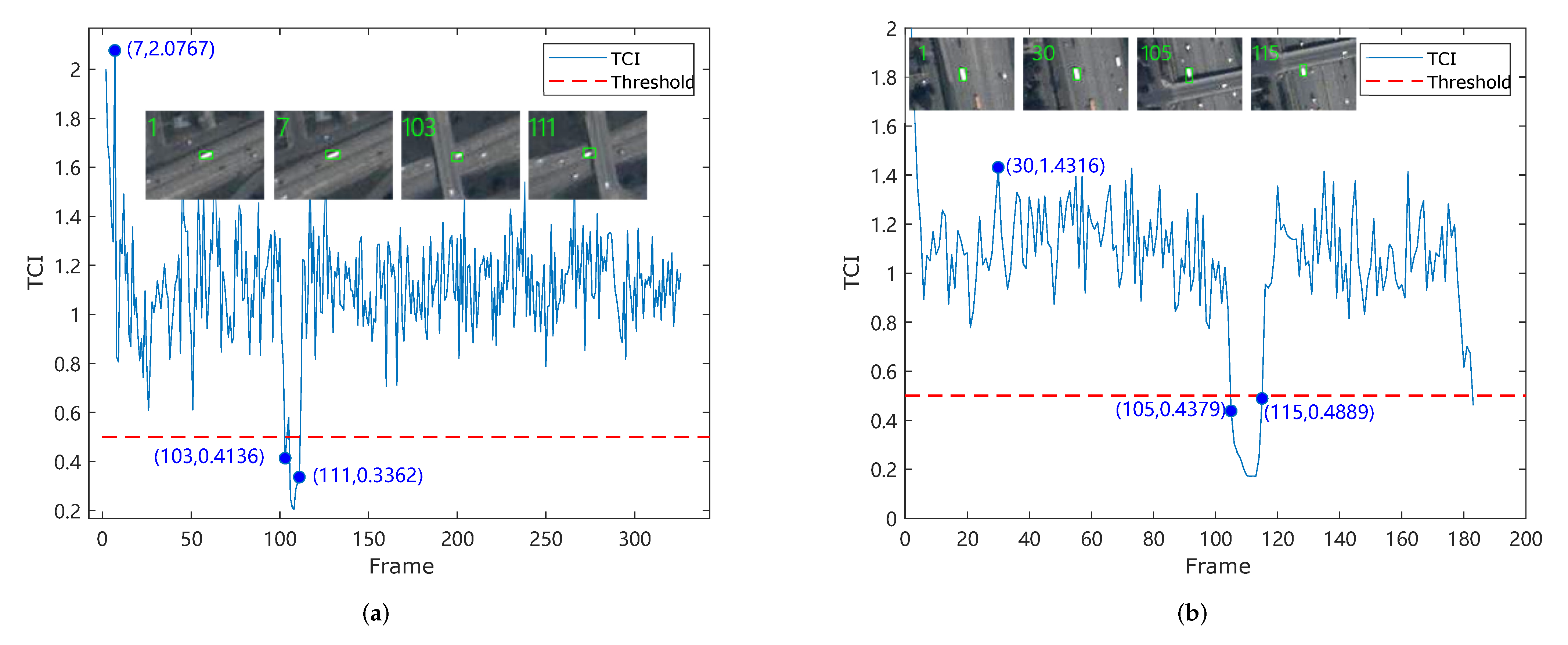
3.1. Tracking Confidence Module

The tracker based on a correlation filter generally adopts the strategy of updating the filter template frame by frame. When the object is partially or completely occluded, the learned filter template will accumulate background information and eventually lead to the loss of the object. Therefore, it is important to accurately judge the tracking status of the object to improve the tracking accuracy.

In the article [23], the author uses the peak response as a criterion to judge whether the tracking process is credible, which can be obtained from Formula (11), and $F_{max}$ is used here to represent the peak response of the response map. However, the peak response can not fully reflect the oscillation degree of the response map, that is, when the object is occluded, the peak response may not be at a low level. Therefore, only using the peak response as an indicator cannot accurately determine whether the object is occluded. Wang et al. proposed the average peak correlation energy ($APCE$), which is used to measure the oscillation degree of the response map [29]. $APCE$ is defined as:

$$APCE=\frac{\left|{\left(y_{max}-y_{min}\right)}^2\right|}{mean\left({\sum }_{r,c}{\left(y_{r,c}-y_{min}\right)}^2\right)}$$

(13)

where $y_{max}$, $y_{min}$ and $y_{r,c}$ are the maximum value, the minimum value and the response value at $(r,c)$ in the response map, respectively. $APCE$ can reflect the oscillation degree of the response map, and the peak response can still reflect whether the tracking is reliable to a certain extent. Therefore, a combination of $APCE$ and $F_{max}$ is recommended here to measure the tracking confidence. The tracking confidence index (TCI) is defined as follows:

$$TC{I}_t=\beta \frac{APC{E}_t}{mean\left({\sum }_0^{t}APC{E}_t\right)}+(1-\beta )\frac{F_{max}^t}{mean\left({\sum }_0^t{F}_{max}^t\right)}$$

(14)

where $APC{E}_t$ and $F_{max}^t$ are $APCE$ and peak response of frame t, respectively, and $\beta$ is set to 0.8. If $TC{I}_t$ satisfaction (15) considers that the tracking of frame t is reliable, otherwise it is judged that the object is occluded, and $\gamma$ is the tracking confidence threshold.

$$TC{I}_t\ge \gamma$$

(15)

3.2. Motion Estimation

When the object is occluded, the key information such as the appearance characteristics of the object will be lost. At this time, the position of the object can be predicted with the help of the speed, acceleration, direction and other information of the object movement. The Kalman filter is an efficient algorithm that can optimally estimate the system state according to the observed measurement results. It has simple form and small amount of calculation, so it is suitable for the tasks that require high real-time performance. In this paper, we use the Kalman filter to estimate the speed, position and direction of moving objects in video. The state equation and observation equation of the system can be written as:

$$\left\{\begin{array}{c}{X}_t=A_{t,t-1}{X}_{t-1}+{\omega }_{t-1}\hfill \\ Z_t=H_t{X}_t+v_t\hfill \end{array}\right.$$

(16)

where $X_t$ and $Z_t$ are the state and observation vector of the system at time t, respectively, $A_{t,t-1}$ is the state transition matrix, $H_t$ is the observation matrix, ${\omega }_{t-1}$ is the process noise matrix, and $v_t$ is the observation noise matrix. The prediction equation of the Kalman filter is:

$$\left\{\begin{array}{c}{X}_{t,t-1}=A_{t,t-1}{X}_{t-1}\hfill \\ P_{t,t-1}=A_{t,t-1}{P}_{t-1}{A}_{t,t-1}^T+Q_{t-1}\hfill \end{array}\right.$$

(17)

The update equation of the Kalman filter is:

$$\left\{\begin{array}{c}{K}_t=P_{t,t-1}{H}_t^T{(H_t{P}_{t,t-1}{H}_t^T+R_t)}^{-1}\hfill \\ X_t=X_{t,t-1}+K_t(Z_t-H_t{X}_{t,t-1})\hfill \\ P_t=(I_t-K_t{H}_t)P_{t,t-1}\hfill \end{array}\right.$$

(18)

where $X_{t,t-1}$ is the state prediction at t time, $X_{t-1}$ is the best estimate of $t-1$ time, $P_{t,t-1}$ is the state covariance matrix at t time, $Q_{t-1}$ is the noise covariance matrix of ${\omega }_{t-1}$, $R_t$ is the measurement noise covariance matrix of $v_t$, $K_t$ is the Kalman gain matrix, and $Z_t$ is the input variable matrix at t time.

Because the change of position between adjacent frames of video is short, the motion of the object can be regarded as linear motion in a short time. So we set the state transition matrix A and observation matrix H to:

$$A=\left[\begin{array}{cccc}1\hfill & 0\hfill & 1\hfill & 0\hfill \\ 0\hfill & 1\hfill & 0\hfill & 1\hfill \\ 0\hfill & 0\hfill & 1\hfill & 0\hfill \\ 0\hfill & 0\hfill & 0\hfill & 1\hfill \end{array}\right],H=\left[\begin{array}{cccc}1\hfill & 0\hfill & 0\hfill & 0\hfill \\ 0\hfill & 1\hfill & 0\hfill & 0\hfill \end{array}\right]$$

(19)

The convergence of the Kalman filter directly affects its prediction results, and the two key parameters of measurement noise covariance matrix R and process noise covariance matrix Q determine the convergence speed and convergence effect. If R is a fixed value, the greater Q is, the more the measured value is trusted; otherwise, the smaller Q is, the more the predicted value of the model is trusted. Assuming that the noise is stable in the original Kalman filter, Q and R are set as fixed values.

In order to improve the prediction performance of the Kalman filter, we fix the measurement noise covariance matrix R and adaptively adjust the noise covariance matrix according to the tracking state of the object. Specifically, if the object is not occluded, the measurement noise covariance matrix R and the process noise covariance matrix Q in the Kalman filter are respectively set as:

$$R=\left[\begin{array}{cc}2\hfill & 0\hfill \\ 0\hfill & 2\hfill \end{array}\right],Q=\left[\begin{array}{cccc}0.001& 0& 0& 0\\ 0& 0.001& 0& 0\\ 0& 0& 0.001& 0\\ 0& 0& 0& 0.001\end{array}\right]$$

(20)

If the object is occluded, the measurement noise covariance matrix R and the process noise covariance matrix Q in the Kalman filter are set as:

$$R=\left[\begin{array}{cc}2\hfill & 0\hfill \\ 0\hfill & 2\hfill \end{array}\right],Q=\left[\begin{array}{cccc}0.00001& 0& 0& 0\\ 0& 0.00001& 0& 0\\ 0& 0& 0.00001& 0\\ 0& 0& 0& 0.00001\end{array}\right]$$

(21)

Adaptively adjusting the noise covariance matrix according to the state of the object tracking process is helpful to improve the convergence speed and prediction performance of the Kalman filter. This will be explained in the experiment section.

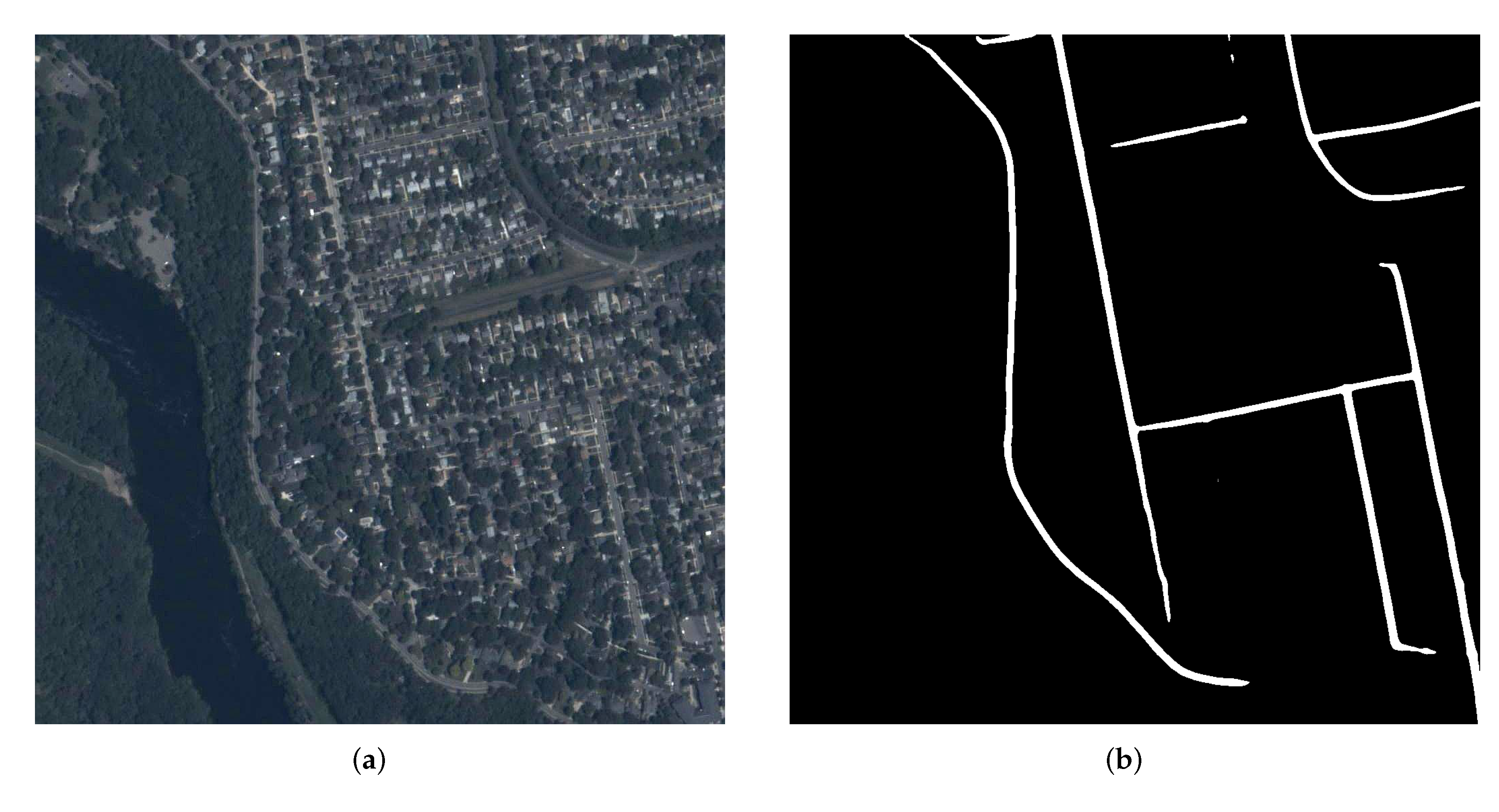
3.3. Object Detection Based on Road Information

Remote sensing images contain abundant road information, which has important applications in emergency response, traffic management, driverless path planning and other fields. For most objects in satellite video, especially vehicle objects, their trajectory usually coincides with the road. Inspired by this, it can be believed that the road information can be used to assist in tracking objects in satellite video. Therefore, an object detection and tracking method under the constraint of road information is proposed in this paper. In order to obtain the road information in the satellite image, we use the method proposed in [30] to extract the road information in the remote sensing image, as shown in Figure 3.

We use the road network picture after binarization as a mask. If a point belongs to a road, the pixel value of the point in the road network picture is 1. If the point does not belong to a road, the pixel value of the point in the road network picture is 0. The overall idea of using road information to assist object tracking is: when it is determined that the object is occluded, firstly stop updating the correlation filter template and use the Kalman filter to predict the position of the object. If the response map of the predicted position satisfies Formula (15), the predicted position of the Kalman filter is used as the position of the object in the current frame. If the response map of the predicted location does not meet Formula (15), select the range of the specified size around the predicted location of the Kalman filter. Assuming that there are N points within the range that belong to the road, take the N points as the center to intercept N image blocks with the same size as the filter template. Use the filter template to perform correlation operations with the N image blocks one by one to obtain N response maps and the corresponding peak response of each response map. We define the maximum of these N peak responses as the local maximum response, which is recorded as $V_{max}$. Further, in order to determine whether $Vmax$ is the corresponding position of the object, the detection threshold (DT) is used as Formula (22):

$$V_{max}>\delta mean\left(\sum _0^t{F}_{max}^t\right)$$

(22)

where $F_{max}^t$ is the max value in the response map of frame t, and $\delta$ is set to 0.5. If $V_{max}$ satisfies (22), it is considered that the object has been successfully detected, and the position corresponding to $V_{max}$ is used as the position of the object in the current frame. If this formula is not satisfied, it is considered that the occlusion state of the object has not yet ended. At this time, the predicted position of the Kalman filter is still used as the position of the object in the current frame.

It can be seen from the above that setting the range of the search area is very important. If the search area is set too small, the actual position of the object may not be included in the search area. If the search area is too large, the traversal process will reduce the tracking efficiency. As mentioned above, the prediction result of the Kalman filter is closely related to its convergence, so in order to evaluate the convergence of the Kalman filter, we use the distance between the predicted position of the Kalman filter and the tracking position of the KCF to judge whether the Kalman filter has been fitted. As shown in Formula (23), when the distance between the predicted position of the Kalman filter and the position tracked by the KCF is less than 2 pixels, the Kalman filter is considered to have been fitted.

$$\sqrt{{(X_{KCF}-X_{KF})}^2-{(Y_{KCF}-Y_{KF})}^2}\le 2$$

(23)

Assuming that the object is occluded at time t, the object position predicted by the Kalman filter is $(X_{KF},Y_{KF})$, and the object speed is $(V_x,V_y)$. When the Kalman filter is fitting, we use the speed predicted by the Kalman filter to determine the search range after the object disappears, as shown in Figure 4a. Figure 4b can visually reflect the object search range assisted by road information. The size of the search range is calculated by the following formula:

$$\left\{\begin{array}{c}X\in (X_{KF}-\frac{{ϵ}_1}{2}{V}_x,X_{KF}+{ϵ}_1{V}_x)\\ Y\in (Y_{KF}-\frac{{ϵ}_2}{2}{V}_y,Y_{KF}+{ϵ}_2{V}_y)\end{array}\right.$$

(24)

$(X,Y)$ is the possible position of the object, and ${ϵ}_1,{ϵ}_2$ is the scale factor. If $V_x>V_y$, then ${ϵ}_1,{ϵ}_2$ are set to 10 and 8, respectively; otherwise, if $V_x\le V_y$, then ${ϵ}_1,{ϵ}_2$ are set to 8 and 10, respectively.

When the Kalman filter is not fitted, the speed obtained by the Kalman filter is not reliable, so the search range is set to a fixed value according to experience as (25), and the settings for ${ϵ}_1$ and ${ϵ}_2$ are the same as Formula (24).

$$\left\{\begin{array}{c}X\in (X_{KF}-\frac{{ϵ}_1}{2},X_{KF}+{ϵ}_1)\\ Y\in (Y_{KF}-\frac{{ϵ}_2}{2},Y_{KF}+{ϵ}_2)\end{array}\right.$$

(25)

4. Experiments

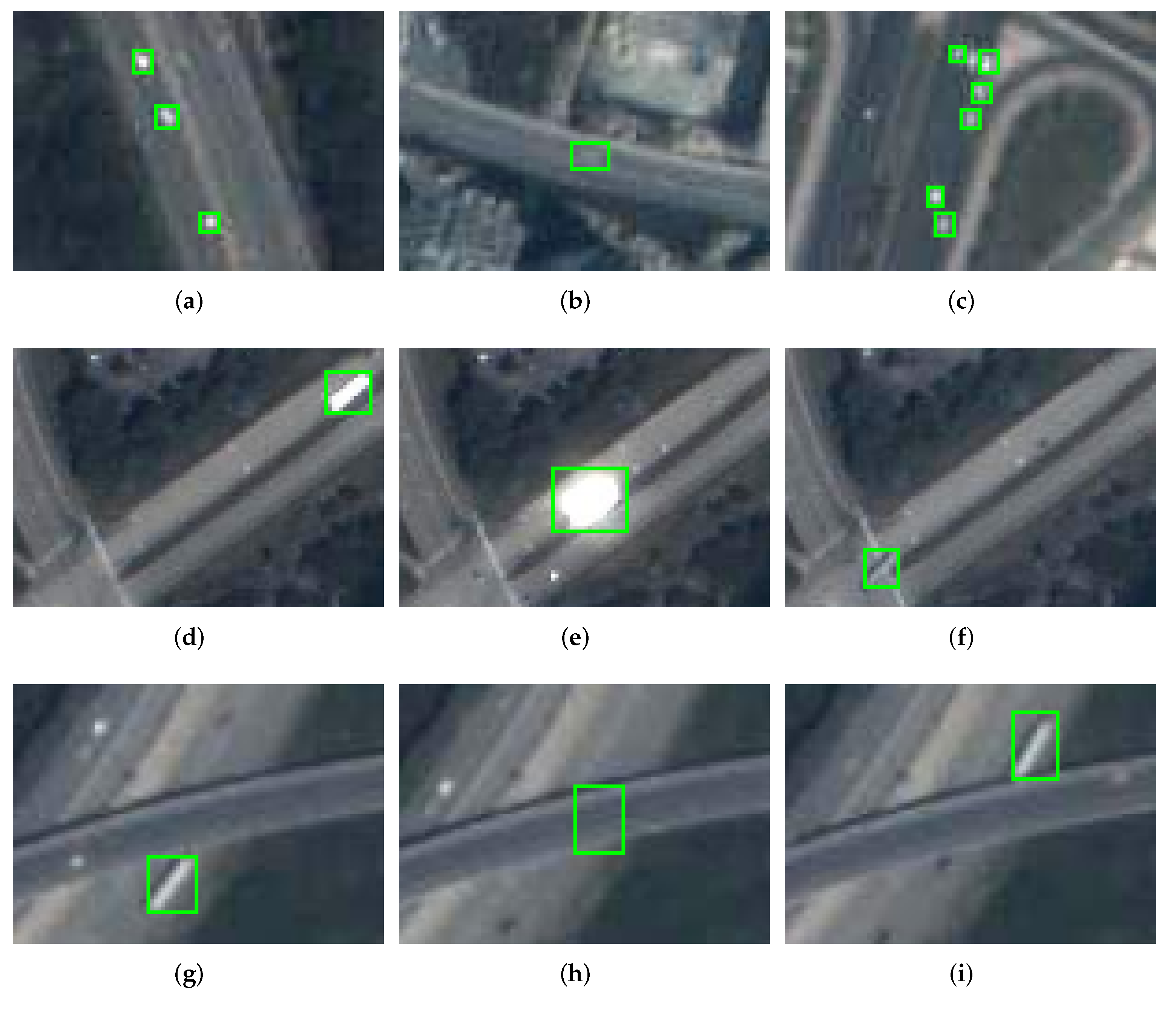
4.1. Datasets and Compared Tracker

The data set used in this paper is from the Jilin-1 satellite. The objects in the video are marked by [31]. We select eight video sequences to compare the tracking performance of our method with that of the comparison method. Each video contains one designated object, all of which are motor vehicles. For more information about the objects, see

Table 1. Overview of the satellite videos and the objects in the experiments.

Sequences	Object Size	Total Number of Frames	Effective Number of Frames	Challenges
1	$13\times 7$	326	322	FOC,TO
2	$11\times 18$	183	179	FOC,TO
3	$9\times 13$	250	250	LQ
4	$19\times 15$	180	180	IV,ROT,DEF
5	$5\times 12$	326	326	POC,TO
6	$9\times 12$	326	320	IV,TO,ROT,FOC,DEF
7	$7\times 7$	300	300	LQ,ROT,TO
8	$7\times 7$	181	181	TO,ROT

. It should be noted that the exact position of the object after it is completely occluded is not provided, so we set the ground truth of the object in the occluded frame to (1,1,1,1), and define the object occluded frame as an invalid frame. The effective frames in Table 1 are obtained by subtracting the invalid frames from the total frames, but the total frames are still used for calculation in the evaluation process. The object size refers to the size of the object in the first frame of the video sequence. For the definition of challenges, reference is made to [32], and the definition is shown in

Table 2. The definition of the challenges.

Attribute	Definition
IV	Illumination Variation: the illumination of the object region changes significantly
FOC	Full Occlusion: the object is fully occluded in the video
LQ	Low Quality: the image is low quality and the object is difficult to be distinguished
ROT	Rotation: the object rotates in the video
DEF	Deformation: non-rigid object deformation
POC	Partial Occlusion: the object is partially occluded in the video
TO	Tiny Object: at least one ground truth bounding box has less than $10\times 10$ pixels

.

We choose CSK tracker [2], CN tracker [4], KCF tracker [3], fDSST tracker [7], STRCF tracker [9], ECO tracker [11] and GFSDCF tracker [12] to compare the tracking performance with the method proposed in this paper. The CSK tracker introduces a cyclic shift strategy based on the MOSSE tracker. The CN tracker uses the color name feature to represent the object. The KCF tracker is a classical correlation filter tracker, which is also the basis of the proposed method. The fDSST tracker can estimate the scale change of the object, and the STRCF tracker adapts well to the changes of the appearance of the object. The ECO tracker and the GFSDCF tracker both use the deep feature. We will verify the performance superiority of the proposed method by comparing it with other trackers.

4.2. Setting of Parameters

All algorithms are carried out on MATLAB 2021. The experimental environment is a Windows 11 system, the Central Processing Unit (CPU) is 2.90 GHz AMD R7-4800h, and the Graphics Processing Unit (GPU) is Nvdia RTX 2060. In the proposed method, the regularization factor $\lambda$ is set to ${10}^{-4}$, the learning rate $\eta$ is set to 0.012, the search area size is 2.5 times the object size, and the $\delta$ in (22) is set to 0.5. Because the object in the satellite video is small, we set the cell size of the HOG feature used in our method and the KCF tracker to $1\times 1$. Because both the ECO tracker and the GFSDCF tracker use the deep feature, these two trackers run using GPU.

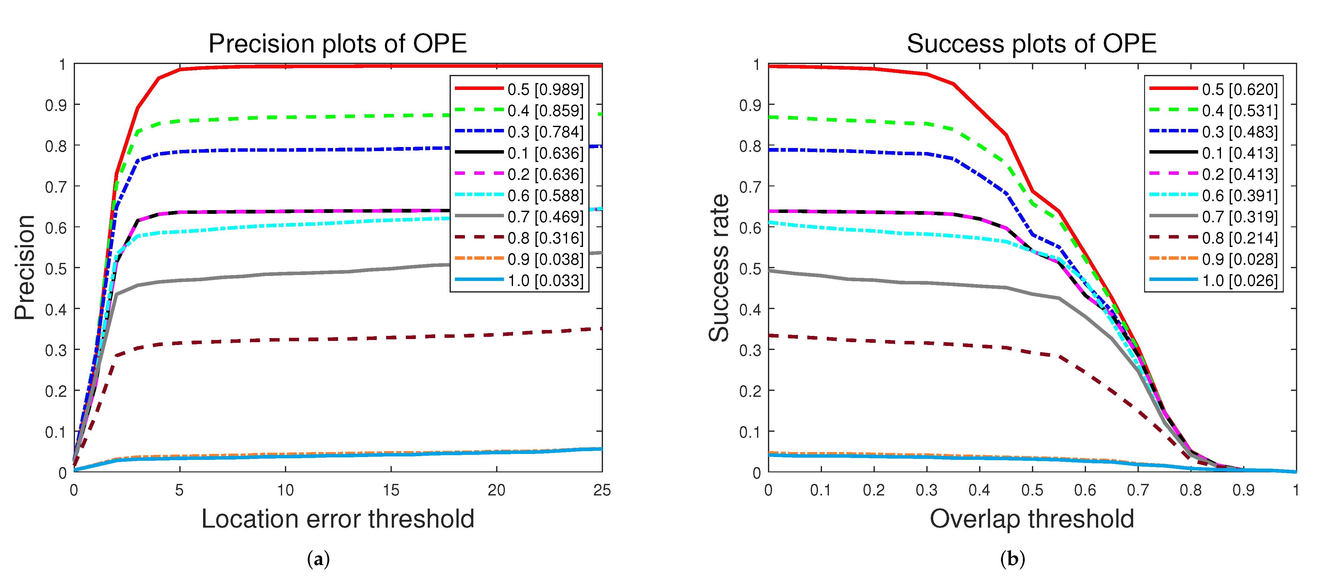
4.3. Evaluation Metrics

In this paper, two commonly recognized metrics [33] are used to quantitatively analyze the object tracking results, namely, the tracking precision score and the tracking success score. In addition, FPS represents the number of frames that the tracker can complete processing per second, which can be used to evaluate the tracking speed of the tracker.

The tracking precision score is defined as the ratio of the number of frames whose center location error (CLE) is less than a certain threshold to the total number of frames. The calculation formula of the center position error is:

$$CLE=\sqrt{{\left(x_p-x_{gt}\right)}^2+{\left(y_p-y_{gt}\right)}^2}$$

(26)

where $(x_p,y_p)$ is the object center position predicted by the tracker, and $(x_{gt},y_{gt})$ is the real position of the object center. Since the object in the satellite is small, the threshold is set to 5 pixels, that is, if the distance between the predicted position and the real position is less than 5 pixels, the tracking is considered successful.

The tracking success score is defined as the ratio of the number of frames whose overlap rate exceeds a certain threshold to the total number of frames. The calculation formula of overlap rate is:

$$S=\frac{\mathrm{Area}\left|r_p\cap r_{gt}\right|}{\mathrm{Area}\left|r_p\cup r_{gt}\right|}$$

(27)

where $r_p$ and $r_{gt}$ refer to the predicted object region and the real object region, respectively, ∩ and ∪ refer to intersection and union, respectively, and ‖ refers to pixels in the region. The overlap rate threshold is set to 0.5, that is, if the overlap rate of the current frame is greater than 0.5, the tracking is considered successful. In the actual evaluation process, the area under curve (AUC) score is generally used as the evaluation index; $\mathrm{AUC}$ refers to the area under the overlap rate curve.

5. Results and Analysis

5.1. Threshold of Occlusion

As mentioned above, we judge whether the object is occluded by observing the TCI fluctuation. Therefore, the selection of threshold has an important impact on whether the tracker can accurately judge the tracking state. We plot the TCI of all video sequences, as shown in Figure 5.

As shown in Figure 5, the TCI value distribution of all sequences can be seen to have an obvious unimodal distribution. Therefore, we can judge whether the object is in an occluded or non occluded state by selecting an appropriate threshold.

In order to select the appropriate threshold $\gamma$, we perform grid search from [0.1, 0.2, 0.3, 0.4, 0.5, 0.6, 0.7, 0.8, 0.9, 1.0] for the threshold $\gamma$. The corresponding tracking precision score and AUC score are shown in Figure 6. It can be seen that when the threshold is 0.5, the tracking precision score and AUC score are the highest, so we set the occlusion threshold $\gamma$ to 0.5.

The visualization of the tracking process of sequences Seq1 and Seq2 in Figure 7 show the relationship between tracking confidence index and object tracking status well. When the threshold is 0.5, it can accurately judge whether the object is occluded. When the object is occluded, TCI is less than the threshold; when the object is not occluded, TCI is greater than the threshold. In a very small number of cases, the object is occluded but the TCI is still greater than the threshold, which is usually caused by illumination change or rapid movement. As can be seen from Figure 7, the duration of this situation is very short, so its impact on the final tracking results can be ignored.

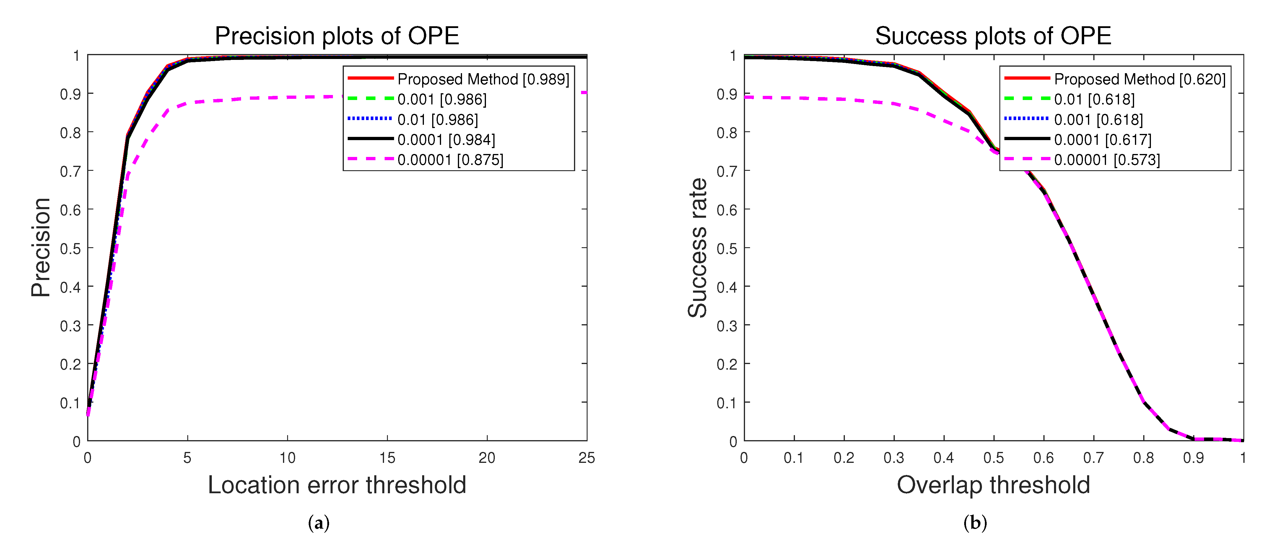
5.2. Noise Covariance Matrix

As mentioned above, the measurement noise covariance matrix R and the process noise covariance matrix Q in the original Kalman filter are fixed values. However, in the practical application, the confidence level of the measured and predicted values should be dynamic. In this article, we adjust the values of Q based on whether the object is occluded. In order to show the advantage of adaptive adjustment of Q, we conduct a comparative experiment by fixing R and adjusting the value of Q. We perform grid search from [0.01, 0.001, 0.0001, 0.00001] for the Q, and the parameter setting of the proposed method is shown in (20) and (21). The experimental results are shown in Figure 8 and

Table 3. Results of comparative experiments. The bold digits denote the optimal results.

	Proposed Method	Q = 0.001	Q = 0.01	Q = 0.0001	Q = 0.00001
Precision Score (%)	0.989	0.986	0.986	0.984	0.875
AUC (%)	0.620	0.618	0.618	0.617	0.573
Success Score (%)	0.758	0.752	0.757	0.753	0.748

.

From the experimental results, it can be seen that compared with the fixed value of Q, the adaptive Q adjustment strategy proposed in this paper improves the performance of the proposed tracker.

5.3. Tracking Result Analysis

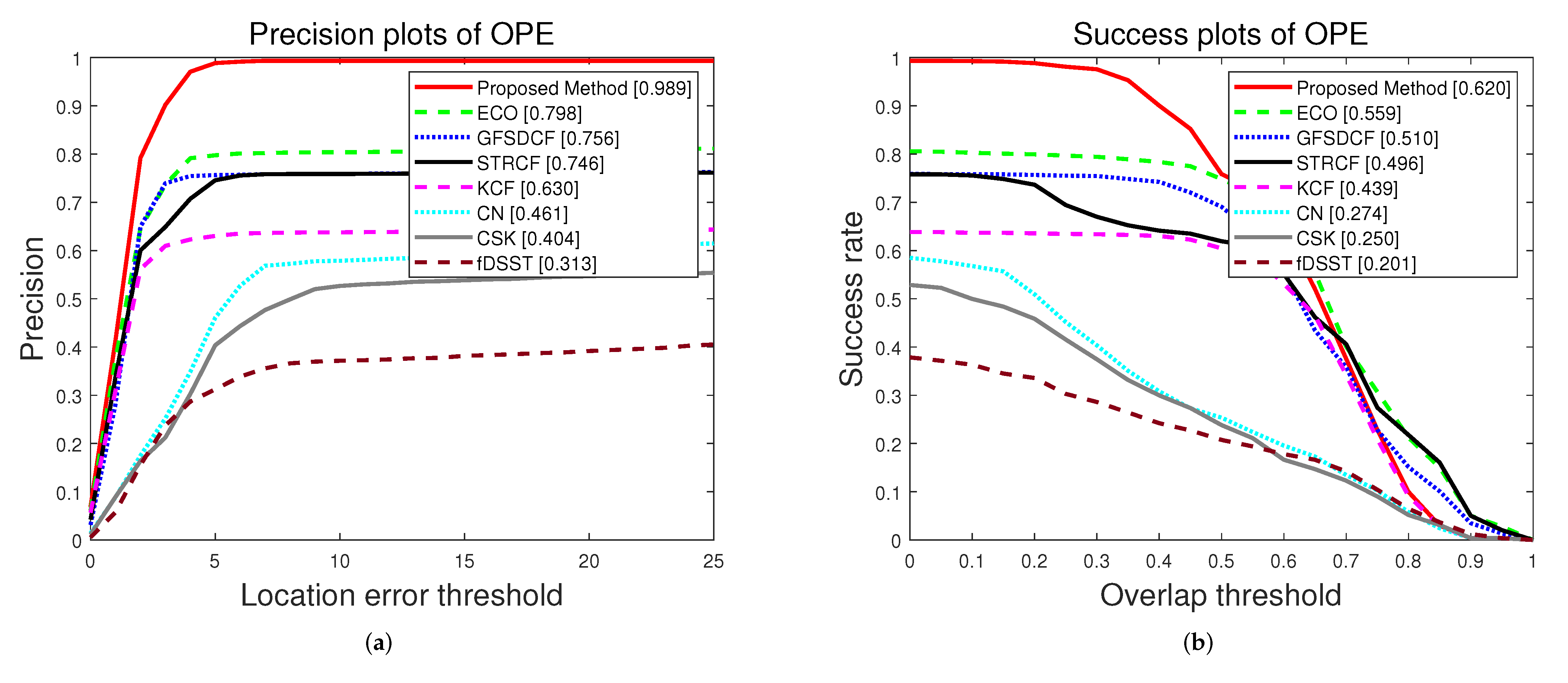
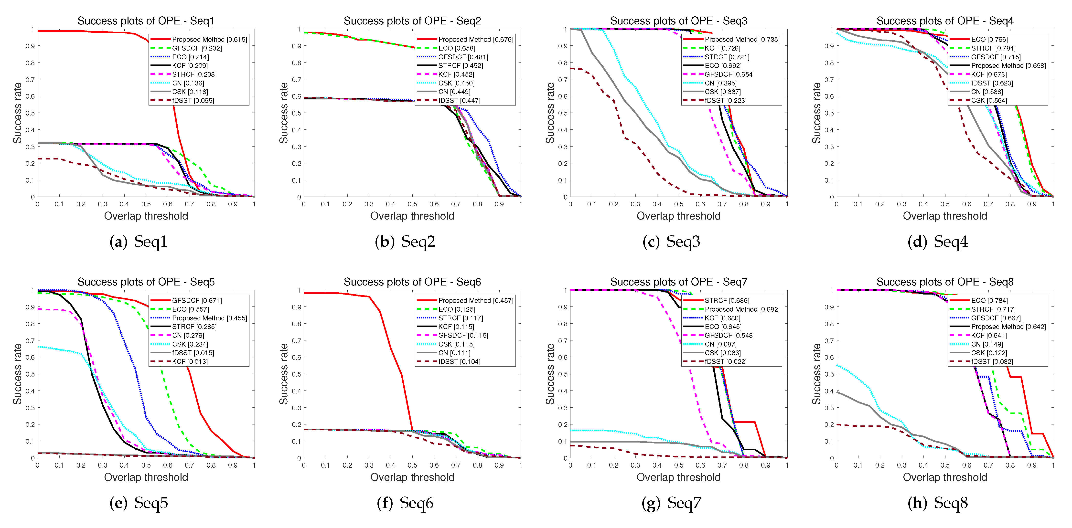
5.3.1. Quantitative Evaluation

Figure 9 shows the tracking precision score and AUC score of the proposed method and the comparison trackers on all sequences. It can be seen that in terms of overall tracking precision score, the proposed method is 19.1% better than the second ranked ECO tracker and 35.9% better than the basic KCF tracker. In terms of overall tracking AUC score, the proposed method is 6.1% better than the second ranked ECO tracker and 18.1% better than the basic KCF tracker.

In order to specifically analyze the performance of each algorithm in different environments, we divide the eight video sequences into five categories according to the motion of the object in the satellite video. In Seq1 and Seq2, the object basically moves along a straight line, and the acceleration is small, which can be regarded as uniform linear motion, but the object is completely occluded during the movement. The objects in Seq3 and Seq4 can also be regarded as moving in a straight line at a constant speed, but they are not affected by occlusion during the movement, and the objects in Seq4 have dramatic changes in appearance due to changes in lighting during the movement. In Seq5, the object is partially occluded in the first frame, and partial occlusion and full occlusion occur many times during the movement. In Seq6, the moving direction of the object changes after it is completely occluded. In Seq7 and Seq8, the object moves nonlinearly but is not blocked during the movement. These objects with different characteristics put forward higher requirements for the comprehensive performance of the algorithm. Figure 10 and Figure 11 show the tracking precision and tracking success AUC of the proposed method and the comparison method on eight satellite video sequences, respectively.

In terms of the tracking precision score, the proposed method has achieved the best results in Seq1, Seq2, Seq5 and Seq6 sequences. Compared with the second ranking tracker, the tracking precision scores of the proposed algorithm in these four sequences have increased by 66.9%, 1.6%, 0.9% and 81.3%, respectively. Compared with the KCF tracker, the tracking precision scores of our method in these four sequences have increased by 66.0%, 38.8%, 97% and 81.3%, respectively. In Seq3, Seq7 and Seq8 sequences, the proposed method achieves a 100% tracking precision score. The tracking precision score of the method in this paper is only 1.5% behind the first ranked tracker in Seq4, but the tracking precision score of our method is still higher than that of the KCF tracker by 2.8%.

In terms of the AUC score, our method has achieved the best results in the Seq1, Seq2, Seq3 and Seq6 sequences. Compared with the second ranked tracker, the AUC scores of our method in these four sequences have increased by 38.3%, 1.8%, 0.9% and 33.2%, respectively. Compared with the KCF tracker, the AUC scores of our method in these four sequences have increased by 40.6%, 22.4%, 0.9% and 34.2%, respectively. The AUC scores of our method on Seq4, Seq5, Seq7 and Seq8 sequences are not the best. However, compared with the KCF tracker, the AUC scores of the proposed method on these four sequences are still increased by 2.5%, 44.2%, 0.2% and 0.1%, respectively. The complete experimental results are shown in

Table 4. The object tracking results of all video sequences employing precision score, AUC score, success score and FPS to determine the best tracker. The bold digits denote the optimal results.

Sequences	Evaluation Metrics	Ours	ECO	GFSDCF	STRCF	KCF	CN	CSK	fDSST
Seq1	Precision score(%)	98.8	31.9	31.9	31.9	31.9	26.7	27.0	20.9
	AUC(%)	61.5	21.4	23.2	20.8	20.9	13.6	11.8	9.5
	Success score(%)	93.6	31.3	31.6	31.3	31.6	9.8	6.7	6.4
	FPS	271	11	5	32	389	872	2669	298
Seq2	Precision score(%)	96.7	95.1	58.5	58.5	57.9	58.5	58.5	58.5
	AUC(%)	67.6	65.8	48.1	45.2	45.2	44.9	45.0	44.7
	Success score(%)	89.1	89.1	57.4	56.8	56.8	56.8	56.8	56.8
	FPS	212	11	5	33	310	1022	3397	335
Seq3	Precision score(%)	100.0	100.0	100.0	100.0	100.0	71.2	56.8	41.6
	AUC(%)	73.5	69.2	65.4	72.1	72.6	39.5	33.7	22.3
	Success score(%)	99.6	99.6	96.4	99.2	99.6	27.2	23.2	4.8
	FPS	478	8	5	33	462	832	2579	249
Seq4	Precision score(%)	98.5	97.9	100.0	95.7	95.7	79.4	75.5	85.6
	AUC(%)	69.8	79.6	71.5	78.4	67.3	58.8	56.4	62.3
	Success score(%)	91.4	96.0	93.6	97.2	87.4	74.5	65.6	77.9
	FPS	107	8	5	33	204	756	2657	241
Seq5	Precision score(%)	98.8	96.3	97.9	93.6	1.8	54.3	46.6	1.8
	AUC(%)	45.5	55.7	67.1	28.5	1.3	27.9	23.4	1.5
	Success score(%)	23.9	79.4	90.8	3.1	1.2	4.0	5.2	1.2
	FPS	384	9	6	33	605	840	3112	289
Seq6	Precision score(%)	98.2	16.9	16.9	16.9	16.9	16.9	16.9	16.9
	AUC(%)	45.7	12.5	11.5	11.7	11.5	11.1	11.5	10.4
	Success score(%)	16.0	16.3	15.6	16.3	16.0	15.6	16.0	12.6
	FPS	261	9	6	35	452	958	3249	285
Seq7	Precision score(%)	100.0	100.0	100.0	100.0	100.0	16.3	9.7	6.0
	AUC(%)	68.2	64.5	54.8	68.6	68.0	8.7	6.3	2.2
	Success score(%)	99.3	89.7	71.7	94.3	97.7	9.3	8.7	0.7
	FPS	540	13	5.3	33	549	716	2197	234
Seq8	Precision score(%)	100.0	100.0	100.0	100.0	100.0	45.3	32.0	18.8
	AUC(%)	64.2	78.4	66.7	71.7	64.1	14.9	12.2	8.2
	Success score(%)	93.9	97.2	95.6	97.2	93.4	5.5	8.3	5.5
	FPS	541	12	5	33	537	693	2196	250

.

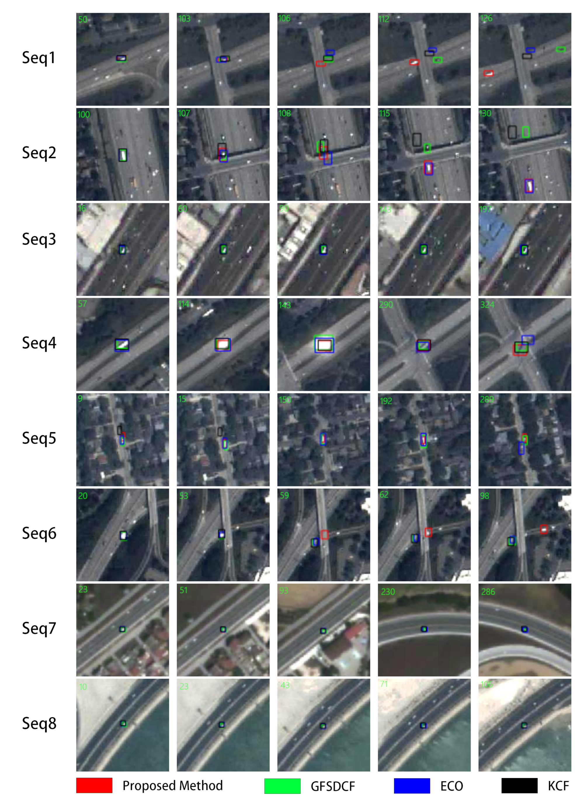
5.3.2. Qualitative Evaluation

In this subsection, we have selected three representative trackers for qualitative evaluation with the trackers proposed in this paper, as shown in Figure 12, where the tracked objects are all moving vehicles. In Seq2, the object is completely occluded in the tracking process. Most of the comparison trackers will lose the object after the object is occluded, while the ECO tracker can continue to track after the object reappears. This came about because the search range of the ECO tracker is larger than the KCF tracker, and the occlusion in the Seq2 sequence is caused by the bridge, its scale is similar to the object size, and the occlusion time is shorter. This enables the ECO tracker to capture the object after it reappears; In Seq1, the object is occluded for a longer time, and the scale of the occluder is larger. Therefore, in Seq1, only the method in this paper can relocate the object and continue to complete the tracking after the object is occluded. In Seq5, the ground truth given by the object in the initial frame is the partially occluded position and size. In the first 10 frames, the object is always partially or completely occluded. At this time, the Kalman filter cannot converge, so the prediction of the object position by the Kalman filter is not credible. Therefore, the object detection module we designed plays a key role in term of object search. The GFSDCF tracker uses the deep feature, so it has more advantages in feature extraction and strong robustness to partial occlusion. The ECO tracker is disturbed by similar objects in the last stage of tracking, which leads to tracking failure. In the most challenging Seq6, the moving direction of the object changes after occlusion. If the Kalman filter is used to predict the position, there is a large deviation in the predicted position. The proposed tracker uses the adaptive Kalman filter and road information to detect the object in time after the object reappears and has achieved good tracking results. However, it should be noted that the proposed method does not detect the rotation and scale change of the object, which makes the tracker match the initial object frame after detecting the object (as shown in frame 98 of Seq6 sequence in Figure 12) and cannot adapt to the direction change of the object and the resulting scale change. Therefore, the AUC score of our method is not high for the object in Seq6. In the sequence without occlusion, the performance of this tracker is close to that of other trackers in Seq3, Seq7 and Seq8. In Seq4, the object is deformed due to the change of illumination in motion. It can be seen clearly in frames 114 and 143 of Seq4 in Figure 12. Since our method is based on the KCF tracker and does not include the scale change of the object in the tracking process, the bounding box cannot match the real size of the object after the object is deformed better. Both the ECO tracker and the GFSDCF tracker can respond to deformation, which can also be reflected in Seq7 and Seq8 sequences. In addition, the 290th frame of Seq4 also reflects the change of brightness under the influence of illumination. It can be seen that the object changes from light to dark. At this time, except for the proposed method, other trackers have tracking drift.

In general, the visualization results show that our method can solve the problem that the object is completely occluded when moving along a straight line. At the same time, it can also solve the problem of unreliable tracking before the Kalman filter is converging and the problem that the moving direction of the object changes after occlusion.

6. Conclusions

In order to solve the problem of object occlusion in satellite video object tracking, we use the road information contained in remote sensing images and propose an improved kernel correlation filter assisted by road information to track small objects in satellite videos. Compared with other methods, the proposed method enjoys the following advantages: Firstly, the reliability of the tracking results of the kernel correlation filter is evaluated by the tracking confidence module.Then, the motion state of the object is estimated by the adaptive Kalman filter. Finally, the object detection module assisted by road information is used to locate and detect the object more accurately. By comparing our tracker with the existing object trackers on the eight video sequences obtained from the Jilin-1 satellite constellation, our tracker achieves the highest tracking precision score on seven sequences and the highest AUC score on four sequences. The result shows that our method is able to effectively solve the problem of tracking failure caused by object occlusion. However, the rotation and scale change of the object are not considered in the proposed method, which leads to it not obtaining a good AUC score, and the problem will be handled in our future work.

References

1. Bolme, D.S.; Beveridge, J.R.; Draper, B.A.; Lui, Y.M. Visual object tracking using adaptive correlation filters. In Proceedings of the Twenty-Third IEEE Conference on Computer Vision and Pattern Recognition, CVPR 2010, San Francisco, CA, USA, 13–18 June 2010. [Google Scholar]
2. Henriques, J.F.; Rui, C.; Martins, P.; Batista, J. Exploiting the Circulant Structure of Tracking-by-Detection with Kernels. In Proceedings of the 12th European Conference on Computer Vision Part IV, Florence, Italy, 7–13 October 2012. [Google Scholar]
3. Henriques, J.F.; Caseiro, R.; Martins, P.; Batista, J. High-Speed Tracking with Kernelized Correlation Filters. IEEE Trans. Pattern Anal. Mach. Intell. 2015, 37, 583–596. [Google Scholar] [CrossRef] [PubMed]
4. Danelljan, M.; Khan, F.S.; Felsberg, M.; Weijer, J. Adaptive Color Attributes for Real-Time Visual Tracking. In Proceedings of the IEEE Conference on Computer Vision & Pattern Recognition, Columbus, OH, USA, 23–28 June 2014. [Google Scholar]
5. Yang, L.; Zhu, J. A Scale Adaptive Kernel Correlation Filter Tracker with Feature Integration. In Proceedings of the IEEE European Conference on Computer Vision, Zurich, Switzerland, 6–7 September 2014. [Google Scholar]
6. Danelljan, M.; Häger, G.; Khan, F.S.; Felsberg, M. Accurate Scale Estimation for Robust Visual Tracking. In Proceedings of the British Machine Vision Conference, Nottingham, UK, 1–5 September 2014. [Google Scholar]
7. Danelljan, M.; Häger, G.; Khan, F.S.; Felsberg, M. Discriminative Scale Space Tracking. IEEE Trans. Pattern Anal. Mach. Intell. 2017, 39, 1561–1575. [Google Scholar] [CrossRef] [PubMed]
8. Danelljan, M.; Hger, G.; Khan, F.S.; Felsberg, M. Learning Spatially Regularized Correlation Filters for Visual Tracking. In Proceedings of the IEEE International Conference on Computer Vision (ICCV), Santiago, Chile, 7–13 December 2015. [Google Scholar]
9. Li, F.; Tian, C.; Zuo, W.; Zhang, L.; Yang, M.H. Learning Spatial-Temporal Regularized Correlation Filters for Visual Tracking. In Proceedings of the 2018 IEEE/CVF Conference on Computer Vision and Pattern Recognition (CVPR), Salt Lake City, UT, USA, 18–22 June 2018. [Google Scholar]
10. Danelljan, M.; Robinson, A.; Khan, F.S.; Felsberg, M. Beyond Correlation Filters: Learning Continuous Convolution Operators for Visual Tracking; Springer International Publishing: Cham, Switzerland, 2016. [Google Scholar]
11. Danelljan, M.; Bhat, G.; Khan, F.S.; Felsberg, M. ECO: Efficient Convolution Operators for Tracking. In Proceedings of the IEEE Conference on Computer Vision and Pattern Recognition, Honolulu, HI, USA, 21–26 July 2017. [Google Scholar]
12. Xu, T.; Feng, Z.H.; Wu, X.J.; Kittler, J. Joint Group Feature Selection and Discriminative Filter Learning for Robust Visual Object Tracking. In Proceedings of the IEEE/CVF International Conference on Computer Vision, Seoul, Korea, 27 October–2 November 2019. [Google Scholar]
13. Held, D.; Thrun, S.; Savarese, S. Learning to Track at 100 FPS with Deep Regression Networks. In Proceedings of the European Conference Computer Vision (ECCV), Amsterdam, The Netherlands, 11–14 October 2016. [Google Scholar]
14. Tao, R.; Gavves, E.; Smeulders, A.W. Siamese instance search for tracking. In Proceedings of the IEEE Conference on Computer Vision and Pattern Recognition, Las Vegas, NV, USA, 27–30 June 2016; pp. 1420–1429. [Google Scholar]
15. Bertinetto, L.; Valmadre, J.; Henriques, J.F.; Vedaldi, A.; Torr, P.H. Fully-convolutional siamese networks for object tracking. In Proceedings of the European Conference on Computer Vision, (ECCV), Amsterdam, The Netherlands, 11–14 October 2016; Springer: Berlin/Heidelberg, Germany, 2016; pp. 850–865. [Google Scholar]
16. Li, B.; Yan, J.; Wu, W.; Zhu, Z.; Hu, X. High performance visual tracking with siamese region proposal network. In Proceedings of the IEEE Conference on Computer Vision and Pattern Recognitio, Salt Lake City, UT, USA, 18–22 June 2018; pp. 8971–8980. [Google Scholar]
17. Li, B.; Wu, W.; Wang, Q.; Zhang, F.; Xing, J.; Yan, J. Siamrpn++: Evolution of siamese visual tracking with very deep networks. In Proceedings of the IEEE/CVF Conference on Computer Vision and Pattern Recognition, Long Beach, CA, USA, 15–20 June 2019; pp. 4282–4291. [Google Scholar]
18. Chen, Z.; Zhong, B.; Li, G.; Zhang, S.; Ji, R. Siamese box adaptive network for visual tracking. In Proceedings of the IEEE/CVF Conference on Computer Vision and Pattern Recognition, Seattle, WA, USA, 14–19 June 2020; pp. 6668–6677. [Google Scholar]
19. Du, B.; Sun, Y.; Cai, S.; Wu, C.; Du, Q. Object Tracking in Satellite Videos by Fusing the Kernel Correlation Filter and the Three-Frame-Difference Algorithm. IEEE Geosci. Remote Sens. Lett. 2018, 5, 168–172. [Google Scholar] [CrossRef]
20. Shao, J.; Du, B.; Wu, C.; Zhang, L. Tracking Objects From Satellite Videos: A Velocity Feature Based Correlation Filter. IEEE Trans. Geosci. Remote Sens. 2019, 57, 7860–7871. [Google Scholar] [CrossRef]
21. Shao, J.; Du, B.; Wu, C.; Zhang, L. Can We Track Targets From Space? A Hybrid Kernel Correlation Filter Tracker for Satellite Video. IEEE Trans. Geosci. Remote Sens. 2019, 57, 8719–8731. [Google Scholar] [CrossRef]
22. Guo, Y.; Yang, D.; Chen, Z. Object Tracking on Satellite Videos: A Correlation Filter-Based Tracking Method With Trajectory Correction by Kalman Filter. IEEE J. Select. Top. Appl. Earth Observat. Remote Sens. 2019, 2, 3538–3551. [Google Scholar] [CrossRef]
23. Xuan, S.; Li, S.; Han, M.; Wan, X.; Xia, G.S. Object Tracking in Satellite Videos by Improved Correlation Filters With Motion Estimations. IEEE Trans. Geosci. Remote Sens. 2019, 58, 1074–1086. [Google Scholar] [CrossRef]
24. Xuan, S.; Li, S.; Zhao, Z.; Zhou, Z.; Gu, Y. Rotation Adaptive Correlation Filter for Moving Object Tracking in Satellite Videos. Neurocomputing 2021, 438, 94–106. [Google Scholar] [CrossRef]
25. Liu, Y.; Liao, Y.; Lin, C.; Jia, Y.; Li, Z.; Yang, X. Object Tracking in Satellite Videos Based on Correlation Filter with Multi-Feature Fusion and Motion Trajectory Compensation. Remote Sens. 2022, 14, 777. [Google Scholar] [CrossRef]
26. Zhang, Y.; Chen, D.; Zheng, Y. Satellite Video Tracking by Multi-Feature Correlation Filters with Motion Estimation. Remote Sens. 2022, 14, 2691. [Google Scholar] [CrossRef]
27. Chen, Y.; Tang, Y.; Yin, Z.; Han, T.; Zou, B.; Feng, H. Single Object Tracking in Satellite Videos: A Correlation Filter-Based Dual-Flow Tracker. IEEE J. Select. Top. Appl. Earth Obs. Remote Sens. 2022, 1–13. [Google Scholar] [CrossRef]
28. Chen, Y.; Tang, Y.; Han, T.; Zhang, Y.; Zou, B.; Feng, H. RAMC: A Rotation Adaptive Tracker with Motion Constraint for Satellite Video Single-Object Tracking. Remote Sens. 2022, 14, 3108. [Google Scholar] [CrossRef]
29. Wang, M.; Yong, L.; Huang, Z. Large Margin Object Tracking with Circulant Feature Maps. In Proceedings of the International Conference on Computer Vision and Pattern Recognition, Venice, Italy, 30 October–1 November 2017. [Google Scholar]
30. Zhou, L.; Zhang, C.; Wu, M. D-LinkNet: LinkNet with pretrained encoder and dilated convolution for high resolution satellite imagery road extraction. In Proceedings of the IEEE Conference on Computer Vision and Pattern Recognition Workshops, Salt Lake City, UT, USA, 18–22 June 2018; pp. 182–186. [Google Scholar]
31. Yin, Q.; Hu, Q.; Liu, H.; Zhang, F.; Wang, Y.; Lin, Z.; An, W.; Guo, Y. Detecting and Tracking Small and Dense Moving Objects in Satellite Videos: A Benchmark. IEEE Trans. Geosci. Remote Sens. 2021, 60, 1–18. [Google Scholar] [CrossRef]
32. Zhao, M.; Li, S.; Xuan, S.; Kou, L.; Gong, S.; Zhou, Z. SatSOT: A Benchmark Dataset for Satellite Video Single Object Tracking. IEEE Trans. Geosci. Remote Sens. 2022, 60, 1–11. [Google Scholar] [CrossRef]
33. Wu, Y.; Lim, J.; Yang, M.H. Object Tracking Benchmark. IEEE Trans. Pattern Anal. Mach. Intell. 2015, 37, 1834–1848. [Google Scholar] [CrossRef] [PubMed] [Green Version]
Figure 1. The problems of tracking objects in satellite videos: (a) small objects; (bf) complex background; (gi) object is occluded.
Remotesensing 14 04215 g001
Figure 2. The flowchart of the proposed method. TCI refers to tracking confidence index, OT and DT refer to occlusion threshold and detection threshold, respectively, and Vmax refers to the maximum response in all response maps.
Remotesensing 14 04215 g002
Figure 3. The remote sensing image and the result of road extraction: (a) is a frame in the satellite remote sensing video; (b) is the corresponding extracted road network map.
Remotesensing 14 04215 g003
Figure 4. Schematic diagram of object speed and search range: (a) is the remote sensing image; (b) is the road network map. The green solid line box is the object boundary box predicted by the Kalman filter, the green dotted line box is the search area, the red arrow represents the object speed along the Y axis, and the blue arrow represents the object speed along the X axis.
Remotesensing 14 04215 g004
Figure 5. TCI value distribution of all frames.
Remotesensing 14 04215 g005
Figure 6. Tracking accuracy score and AUC score obtained by different thresholds: (a) tracking accuracy score plots; (b) tracking AUC score plots.
Remotesensing 14 04215 g006
Figure 7. Visualization of partial tracking results: (a) occlusion process of Seq1 sequences; (b) occlusion process of Seq2 sequences.
Remotesensing 14 04215 g007
Figure 8. Tracking accuracy score and AUC score obtained by different Q: (a) tracking accuracy score plots; (b) tracking AUC score plots.
Remotesensing 14 04215 g008
Figure 9. Experimental results on the eight sequences: (a) tracking accuracy score plots; (b) tracking AUC score plots.
Remotesensing 14 04215 g009
Figure 10. Precision plots of eight video sequences involving object sequences without and with occlusion. The legend in the precision plot is the corresponding precision score per object tracker.
Remotesensing 14 04215 g010
Figure 11. Success plots of eight video sequences involving object sequences without and with occlusion. The legend in the success plot presents the corresponding AUC per object tracker.
Remotesensing 14 04215 g011
Figure 12. Screenshots of some tracking results. At each frame, the bounding boxes with different colors are the tracking results of the different trackers, and the green number in the top-left corner is the frame number of the current frame in the satellite videos.
Remotesensing 14 04215 g012