PGNet: Positioning Guidance Network for Semantic Segmentation of Very-High-Resolution Remote Sensing Images

Abstract

Semantic segmentation of very-high-resolution (VHR) remote sensing images plays an important role in the intelligent interpretation of remote sensing since it predicts pixel-level labels to the images. Although many semantic segmentation methods of VHR remote sensing images have emerged recently and achieved good results, it is still a challenging task because the objects of VHR remote sensing images show large intra-class and small inter-class variations, and their size varies in a large range. Therefore, we proposed a novel semantic segmentation framework for VHR remote sensing images, called Positioning Guidance Network (PGNet), which consists of the feature extractor, a positioning guiding module (PGM), and a self-multiscale collection module (SMCM). First, the PGM can extract long-range dependence and global context information with the help of the transformer architecture and effectively transfer them to each pyramid-level feature, thus effectively improving the segmentation effectiveness between different semantic objects. Secondly, the SMCM we designed can effectively extract multi-scale information and generate high-resolution feature maps with high-level semantic information, thus helping to segment objects in small and varying sizes. Without bells and whistles, the $mIoU$ scores of the proposed PGNet on the iSAID dataset and ISPRS Vaihingn dataset are 1.49% and 2.40% higher than FactSeg, respectively.

1. Introduction

Semantic segmentation, which assigns semantic labels to each pixel of an image, is a pixel-level classification task. In the field of remote sensing, semantic segmentation, also known as the classification of land use and land cover (LULC) types [1], plays an important role in the intelligent interpretation of remote sensing and provides a basis for many remote sensing applications, such as obstacle detection and avoidance [2], urban planning [3,4], disaster assessment [5,6], ecological observation [7,8], and agricultural production [9,10].

With the development of image processing and machine learning technology [11,12,13,14], many methods for semantic segmentation of VHR remote sensing images have been proposed. Existing methods can be divided into two main types: the traditional manual feature-based (TMF-based) method [15,16,17] and the deep learning-based (DL-based) method [3,4,18,19,20,21,22]. The TMF-based method first extracts features based on a potential semantic object’s color, texture, shape, and spatial relationships. It then uses clustering or classification to segment the VHR remote sensing images. Since the TMF-based method highly relies on the manually extracted features, it does not perform well in complex VHR remote sensing images. Unlike the TMF-based methods, the DL-based methods do not rely on manually extracted features. They can automatically extract features at different semantic levels by convolutional neural networks (CNN) or the vision transformer (ViT), achieving higher segmentation accuracy in complex scenes. Therefore, the DL-based methods have attracted more attention and are developing rapidly.

Although many DL-based methods have achieved good segmentation results, it is still challenging because VHR remote sensing images have their characteristics compared to natural images, which can be observed in Figure 1. First, VHR remote sensing images tend to exhibit large intra-class and small inter-class variations at the semantic-object-level due to the diversity and complexity of ground objects [9]. Second, although VHR remote sensing images are rich in details, the objects are generally small in the background and are easily lost after repeated downsampling [3,9]. Third, the objects in VHR remote sensing images have a large variation in size, which easily leads to unstable segmentation performance, i.e., it cannot maintain good performance for small and large objects [11,22,23].

Therefore, we proposed a novel semantic segmentation framework for VHR remote sensing images called Positioning Guidance Network (PGNet), which is composed of three parts: a feature extractor, a positioning guidance module (PGM), and a self-multiscale collection module (SMCM). To address the challenge of large intra-class and small inter-class variations of semantic objects in VHR remote sensing images, we proposed PGM to obtain a long-range dependence to solve the problem of small inter-class variations and obtain global context information to solve the problem of large intra-class variations. Specifically, PGM can obtain long-range dependence and global context information through the transformer architecture, efficiently propagating this information to each pyramid-level feature. To address the challenge that objects in VHR remote sensing images are small and vary in size, we proposed SMCM to collect multiscale information while acquiring high-resolution feature maps with high-level semantic information.

Our main contributions are summarized below:

• To the best of our knowledge, the proposed PGNet is the first to efficiently propagate the long-range dependence obtained by ViT to all pyramid-level feature maps in the semantic segmentation of VHR remote sensing images.
• The proposed PGM can effectively locate different semantic objects and then effectively solve the problem of large intra-class and small inter-class variations in VHR remote sensing images.
• The proposed SMCM can effectively extract multiscale information and then stably segment objects at different scales in VHR remote sensing images.
• We conducted extensive experiments on two challenging VHR remote sensing datasets, the iSAID [24] dataset and the ISPRS Vaihingen [25] dataset, to demonstrate the excellent segmentation performance of PGNet.

The rest of this paper is organized as follows. Section 2 introduces the related work on the semantic segmentation of VHR remote sensing images and vision transformer. Section 3 describes the overall framework and important components of PGNet. Section 4 provides the experiments and analysis on the iSAID dataset and ISPRS Vaihingen dataset. The conclusion of this paper is in Section 5.

2. Related Work

We first review the semantic segmentation methods of VHR remote sensing images. Then we review the vision transformer, which is closely related to our work.

2.1. Semantic Segmentation of VHR Remote Sensing Images

The semantic segmentation of VHR remote sensing images plays an important role in remote sensing image understanding. Many excellent semantic segmentation methods for VHR remote sensing images have emerged in recent years. These methods can be divided into the traditional manual feature-based (TMF-based) methods and the deep-learning-based (DL-based) methods.

Traditional manual feature-based method. The TMF-based methods first extract features based on a potential semantic object’s color, texture, shape, and spatial relationships and then use clustering or classification algorithms to segment the images. Cheng et al. [15] proposed an LBP-based segmentation method that combines statistical region merging (SRM) and regional homogeneity local binary pattern (RHLBP) for initial segmentation and uses a support-vector machine (SVM) for semantic category classification. Zhang et al. [16] generated the initial segmentation by the local best region growth process, and then the local mutual best region merging process was applied to a region adjacency graph (RAG) for segmentation. Wang et al. [17] proposed a combination of superpixels and minimum spanning tree for VHR remote sensing image segmentation. The TMF-based methods may fail in complex situations because they highly rely on manually extracted features.

Deep learning-based method. The DL-based method does not rely on hand-extracted features. It can automatically extract features at different semantic levels, such as discriminative feature learning [26,27], so it can achieve high accuracy segmentation resulting in complex VHR remote sensing images. In recent years, many DL-based semantic segmentations of VHR remote sensing images have been proposed [3,4,18,19,20,21,22,28,29,30,31,32,33]. Some of these works focus on improving the semantic segmentation performance of VHR remote sensing images based on transfer learning [28,29,30,31,32]. Cui et al. [28] were inspired by transfer learning and designed TL-DenseUNet, which achieves good performance even with insufficient and unbalanced labeled training. Some previous works have focused on improving the network architecture to increase performance [3,4,18,19,20,21,22,33]. Diakogiannis et al. [33] proposed ResUNet, which employs UNet with residual convolutional blocks as the segmentation backbone and combines atrous convolution and pyramid scene parsing (PSP) pooling to aggregate the context information. Ma et al. [3] propose FactSeg, a symmetrical dual-branch decoder consisting of a foreground activation branch and a semantic refinement branch. The two branches perform multiscale feature fusion through skip connection, thereby improving the segmentation accuracy of small objects. Li et al. [18] propose MANet to extract contextual dependencies through multiple efficient attention modules, effectively improving the semantic segmentation of VHR remote sensing images. Chen et al. [22] propose the boundary enhancing semantic context network (BES-Net) to use the boundary to enhance semantic context extraction explicitly.

2.2. Transformer in Vision

Motivated by the enormously successful transformer in NLP [34,35], many works have attempted to replace convolutional layers altogether or to combine CNN-like architectures with the transformer for vision tasks [36,37,38] for easier capture of long-range dependence. Following the standard transformer paradigms, Dosovitskiy et al. [36] presented a pure transformer model called vision transformer (ViT), which achieved state-of-the-art (SOTA) results on the image classification task. Wang et al. [39] proposed pyramid vision transformer (PVT), the first pure transformer backbone designed for various pixel-level dense prediction tasks. Liu et al. [40] proposed a hierarchical transformer whose representation is computed with shifted windows. Xie et al. [37] proposed a novel positional-encoding-free and hierarchical transformer encoder, named mix transformer (MiT), which is designed for the semantic segmentation task.

Recently, several semantic segmentation works of VHR remote sensing images have used the transformer as the feature extractor to extract feature maps with long-range dependence efficiently [4,6,8,9]. Wang et al. [9] proposed a two-branch network CCTNet, which combines the local details captured by CNNs with the global context information provided by the transformer. Tang et al. [6] used SegFormer [37], a semantic segmentation model for natural images, for remote sensing image segmentation to achieve landslide detection. He et al. [8] proposed a novel semantic segmentation framework for remote sensing images called the ST-U-shaped network, which embeds the Swin transformer into the classical CNN-based UNet. Ding et al. [4] proposed WiCoNet, a semantic segmentation network combining CNN and Transformer, for fully extracting local and long-range dependence from VHR remote sensing images.

Unlike previous works that extract features directly using the transformer or using a two-branch architecture with a combination of convolutional layers and the transformer, our proposed PGNet uses a convolutional neural network as the feature extractor. Additionally, since long-range dependence can effectively locate different semantic objects [41], we use the transformer architecture on the high-level feature map to extract long-range dependence and propagate this information to each pyramid-level feature.

3. Proposed Method

The overall architecture of the proposed PGNet is illustrated in Figure 2, which consists of three components: the feature extractor, the positioning guidance module (PGM), and the self-multiscale collection module (SMCM). First, the PGM we designed fully uses the long-range dependence extracted by the transformer architecture, which can help locate objects of different semantic classes. At the same time, because this long-range dependence is a kind of global context information, it helps the segmentation of objects with large intra-class variations. Second, the SMCM we designed can extract multi-scale information and obtain high semantic high-resolution feature maps, improving the segmentation results of small and varying-sized objects.

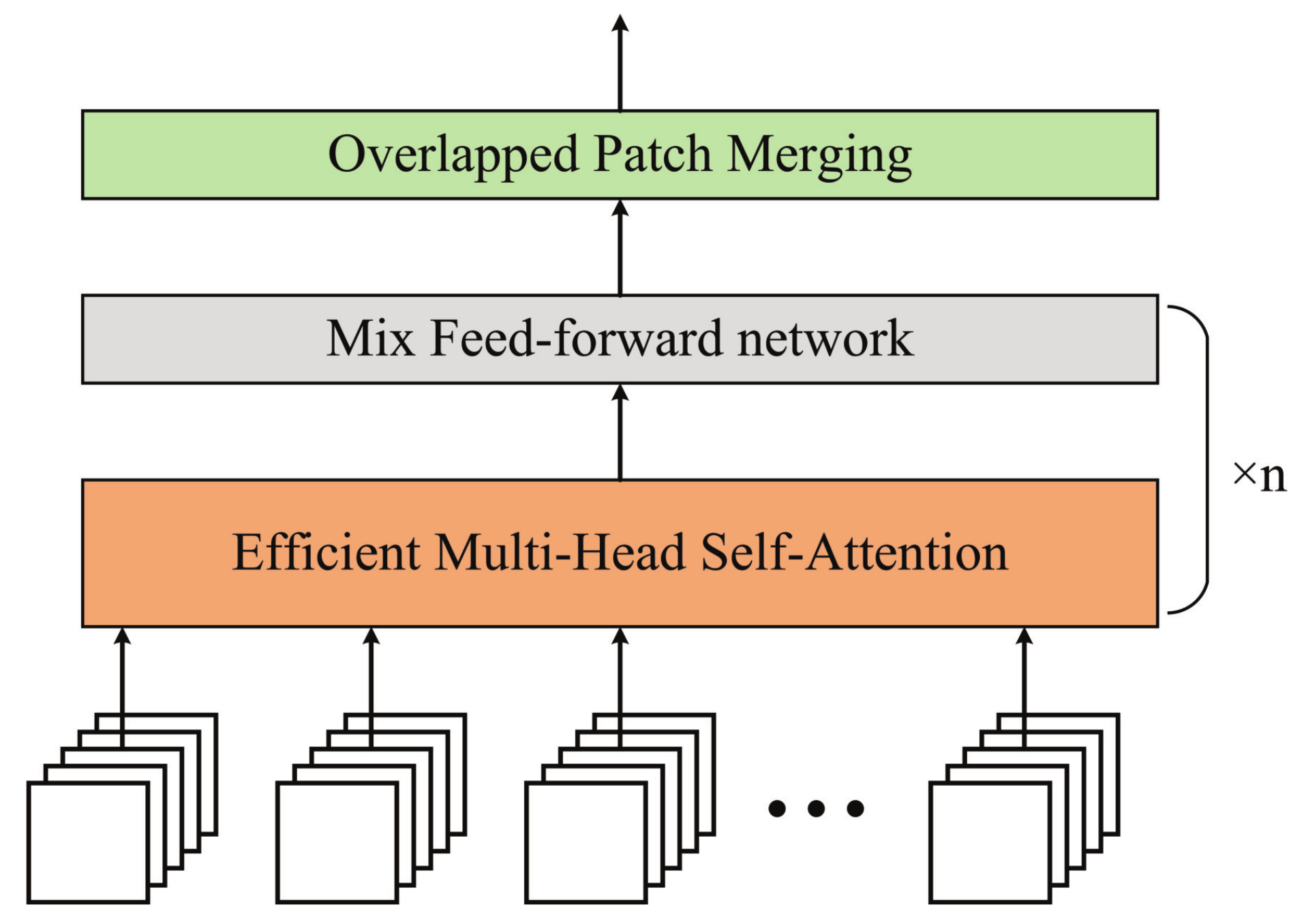
3.1. Feature Extractor

Many studies have shown that pre-trained feature extractors perform well in semantic segmentation tasks [3,42,43]. In particular, the Res2Net [44] architecture with residual module has a powerful feature extraction ability. In the proposed PGNet, Res2Net was used as a feature extractor without fully connected layers. As shown in Figure 2, given an input image $I\in {\mathbb{R}}^{H\times W\times C}$, we fed it into Res2Net to extract features to obtain multi-level feature maps $C_i(i=1,2,3,4)$ at $\left\{\frac{1}{4},\frac{1}{8},\frac{1}{16},\frac{1}{32}\right\}$ of the original image resolution. In addition, the PGNet we proposed is a flexible framework and is not limited to using Res2Net as the feature extractor.

3.2. Positioning Guidance Module

Unlike natural images, the objects in VHR remote sensing images are often characterized by small inter-class and large intra-class variances. Previous works [22,23,41] have demonstrated that long-range dependence can well localize objects with camouflage, while global context information can well segment objects with large intra-class differences. Therefore, we designed the positioning guidance module (PGM) to extract long-range dependence and global context information and efficiently transfer this information to each pyramid-level feature.

The enormous success of the transformer in NLP [34,35] has led many works to replace convolutional layers entirely with the transformer or to combine CNN-like architectures with the transformer for vision tasks, which can easily capture global contextual features and build long-range dependence [37,38,40]. The reason why the transformer architecture can obtain long-range dependence is the use of the multi-head self-attention (MSA) mechanism with query-key-value (QKV) [34], which can be described as follows:

$$\begin{array}{c}MultiHead(Q,K,V)=Concat(hea{d}_1,\dots ,hea{d}_h)W^0\\ hea{d}_i=Attention(Q_i,K_i,V_i)\end{array},$$

(1)

where $Attention(Q_i,K_i,V_i)$ is the self-attention mechanism, as defined in Equation (2).

$$Attention(Q_i,K_i,V_i)=softmax\left(\frac{Q_i{K}_i^T}{\sqrt{D_k}}\right)V_i=A{V}_i,$$

(2)

where $Q_i$ represents the query vector, $K_i$ represents the keyword vectory, $V_i$ represents the content vector, and $\sqrt{D_k}$ represents the scaling factor. For an image, by calculating the dot product of $Q_i$ and $K_i$ for correlation, the correlation matrix between each pixel in the image can be obtained; then, the weight map corresponding to each position is output by the Softmax activation function. Finally, the weight map is superimposed to $V_i$, and the purpose of weighting different regions can be achieved. In this way, the long-range dependence is obtained. Notice that $Q_i$, $K_i$, and $V_i$ are all matrices related to the input content X, as formulated in Equation (3).

$$\left\{\begin{array}{c}{Q}_i=X{W}^{Q_i}\hfill \\ K_i=X{W}^{K_i}\hfill \\ V_i=X{W}^{V_i}\hfill \end{array}.\right.$$

(3)

The above theoretical analysis shows that the transformer architecture can obtain long-range dependence and global context information. Therefore, our PGM uses the long-range dependent information and global information obtained from the transformer architecture to guide the decision process of semantic segmentation. As shown in Figure 2, we used the feature map $C_4$ generated in the last stage of Res2Net as the input to the PGM, as shown in Equation (4).

$$P=PGM\left(C_4\right),$$

(4)

where $PGM(·)$ represents the positioning guidance module, P represents the output result of PGM, which contains three sizes of output $\left\{p_1,p_2,p_3\right\}$.

One of the critical components of PGM is the transformer layer, which is designed based on mix transformer [37]. We first performed dimension reduction of the feature map $C_4$ by Equation (5) from 2048 to 320 dimensions to reduce the number of parameters in the network.

$$\widetilde{C_4}=Con{v}_{1\times 1}\left(C_4\right),$$

(5)

where $Con{v}_{1\times 1}$ represents a $1\times 1$ convolution. Immediately afterwards, we divided $\widetilde{C_4}\in {\mathbb{R}}^{\frac{H}{32}\times \frac{W}{32}\times 320}$ into $4\times 4$-sized patches, denoted as $\widetilde{\tilde{C_4}}\in {\mathbb{R}}^{\frac{HW}{128\times 128}\times (320\times 16)}$. Finally, we passed $\widetilde{\tilde{C_4}}$ through the transformer layer to get the initial positioning guiding flow, which can be written as

$$G=MiTLayer\left(\widetilde{\tilde{C_4}}\right)$$

(6)

where $MiTLayer(·)$ represents a transformer layer, which is based on the mix transformer. The transformer layer is shown in Figure 3 and consists of efficient multi-head self-attention, mix feed-forward network, and overlapped patch merging. Thus, $MiTLayer(·)$ can be described as

$$MiTLayer\left(\widetilde{\tilde{C_4}}\right)=OPM\left(MFFN{\left(ESA\left(\widetilde{\tilde{C_4}}\right)\right)}^n\right)$$

(7)

where $ESA(·)$ represents efficient multi-head self-attention, $MFFM(·)$ represents mix feed-forward network, and $OPM(·)$ means overlapped patch merging. In addition, ${(·)}^n$ denotes n identical operations, where $n=2$.

Efficient multi-head self-attention is essentially the multi-head self-attention, as shown in Equation (1). The difference from the original multi-head self-attention process is the acquisition of K values, which is different from Equation (3). This process uses the reduction ratio R to reduce the length of the sequence as follows:

$$\begin{array}{c}\tilde{K}=\mathrm{Re}shape(\frac{N}{R},C·R)\left(K\right)\hfill \\ K=Linear(C·R,C)\left(\tilde{K}\right)\hfill \end{array},$$

(8)

where K is the sequence to be reduced. $\mathrm{Re}shape(\frac{N}{R},C·R)\left(K\right)$ refers to reshaping K to a shape of $\frac{N}{R}\times (C·R)$, and $Linear(C_{in},C_{out})(·)$ refers to a linear layer taking a $C_{in}$-dimensional tensor as input and generating a $C_{out}$-dimensional tensor as output. Therefore, the new K has dimensions $\frac{N}{R}\times C$. Note that our transformer layer uses an 8-head self-attention and that $R=1$ in Equation (8). Mix-FFN can be formulated as

$$X_{out}=MLP(GELU\left(Con{v}_{3\times 3}\left(MLP\left(X_{in}\right)\right)\right)+X_{in},$$

(9)

where $X_{in}$ is the feature from the self-attention module, $MLP(·)$ is the multilayer perceptron layer, $Con{v}_{3\times 3}(·)$ is a $3\times 3$ convolution, and $GELU(·)$ is a GELU activation function [45].

3.3. Self-Multiscale Collection Module

The objects of VHR remote sensing images are often in small and varying sizes, which hinders the algorithms from generating high-quality semantic segmentation results. Therefore, we proposed a new module called self-multiscale collection module (SMCM), which can obtain high semantic high-resolution feature maps and collect multiscale information. It is well known that high-level feature maps have high-level semantic information but are low-resolution and lack detailed information, while low-level feature maps are the opposite [41]. Many methods are proposed for obtaining high-resolution feature maps with high-level semantic information for better semantic segmentation, such as UNet [46], and FPN [47]. However, our SMCM is different from existing works, as shown in Figure 4. We first took the positioning guiding flow $p_i$, the low-level feature map $C_i$ and the high-level feature map $S_{i+1}$ or $C_4$ as the input of SMCM to obtain the high-resolution feature map $M_i$ with high-level semantic information, where $M_i$ is the intermediate feature map of SMCM. This process can be written as

$$M_i=\left\{\begin{array}{c}(\alpha p_i+C_i)\otimes S_{i+1}+\alpha p_i+C_{i}i=1,2\hfill \\ (\alpha p_i+C_i)\otimes C_{i+1}+\alpha p_i+C_{i}i=3\hfill \end{array},\right.$$

(10)

where ⊗ represents the Hadamard product, and $\alpha$ is a learnable parameter with an initialization value of 1.00. Note that this is all done here with a channel count of 256.

The development of deep convolutional neural networks has seen the emergence of many methods for extracting multi-scale information to ensure good segmentation performance in a large variation in object size, such as ASPP [23] and PPM [48]. However, they are mostly fixed in the deepest layer of the deep neural networks, which is not friendly enough for semantic segmentation of VHR remote sensing images because the object sizes of VHR remote sensing images are often small and may be covered by the background after multiple downsampling. At the same time, this multi-scale information may be diluted in the bottom-to-top path. Therefore, we designed a multi-scale collection strategy based on the human vision principle [49] that humans tend to use zoom-in and zoom-out operations to observe objects of varying sizes.

The implementation of this multi-scale strategy on SMCM is shown in Figure 4, we first obtained three different scales of feature maps $B_i^0$, $B_i^1$, $B_i^2$ from the intermediate feature map $M_i$ by

$$\left\{\begin{array}{c}{B}_i^0=f_{cbr}\left(Up(M_i\right))\hfill \\ B_i^1=f_{cbr}\left(M_i\right)\hfill \\ B_i^2=f_{cbr}\left(Down\left(M_i\right)\right)\hfill \end{array},\right.$$

(11)

where $f_{cbr}(·)$ represents a series of operations in the order of the $1\times 3$ convolution, $3\times 1$ convolution, batch normalization and ReLU activation function. The purpose of using $1\times 3$ convolution and $3\times 1$ convolution here is to reduce the number of parameters in the model. In addition, $Up(·)$ is bilinear interpolation upsampling performed twice, and $Down(·)$ is the average pooling operation with a stride of 2. Then, we interacted with the feature maps at different scales with information as follows:

$$\left\{\begin{array}{c}{\tilde{B}}_i^0=f_{br}(f_c\left(B_i^0\right)+f_c\left(Up\left(B_i^1\right)\right))\hfill \\ {\tilde{B}}_i^1=f_{br}(f_c\left(Down\left(B_i^0\right)\right)+f_c\left(B_i^1\right)+f_c\left(Up\left(B_i^2\right)\right))\hfill \\ {\tilde{B}}_i^2=f_{br}(f_c\left(Down\left(B_i^1\right)\right)+f_c\left(B_i^2\right)))\hfill \end{array},\right.$$

(12)

where $f_{br}$ is the sequential batch normalization and ReLU activation function, and $f_c$ means a series of convolution operations in the order of the $1\times 3$ convolution and $3\times 1$ convolution. Finally, we performed the operation shown in Equation (13) to collect information at different scales to obtain the final output feature map $S_i$, which is the high-resolution feature map with high-level semantic and multi-scale information.

$$S_i=f_{br}(f_c\left(Down\left({\tilde{B}}_i^0\right)\right)+f_c\left({\tilde{B}}_i^1\right)+f_c\left(Up\left({\tilde{B}}_i^2\right)\right)).$$

(13)

Embedding SMCM into the PGNet allows the network to stably segment objects in small and varying sizes in VHR remote sensing images.

3.4. Loss Function

For the final predicted output, we need to operate on feature map $S_1$ as follows:

$$F=Con{v}_{3\times 3}\left(S_1\right),$$

(14)

where F is the final predicted output. In the training phase, our PGNet uses the standard cross-entropy loss as the loss function, which is defined as follows:

$$loss(F,G)=-\frac{1}{N}\sum _{k=1}^N[G_{k}log\left(F_k\right)+(1-G_k)log(1-F_k)],$$

(15)

where G denotes the ground truth, while k is the index of pixels and N is the number of pixels in F.

4. Experiments and Discussions

In this section, we conducted extensive experiments on two different datasets to evaluate the performance of our proposed PGNet. The details of the experimental setup are in Section 4.1. The comparison experiments and analysis of PGNet and SOTA methods on the iSAID and Vaihingen dataset are provided in Section 4.2. The ablation experimental results and analysis of the two core modules of our proposed PGNet, PGM and SMCM, are presented in Section 4.3. The efficiency analysis of the PGNe and SOTA methods is provided in Section 4.4.

4.1. Experimental Settings

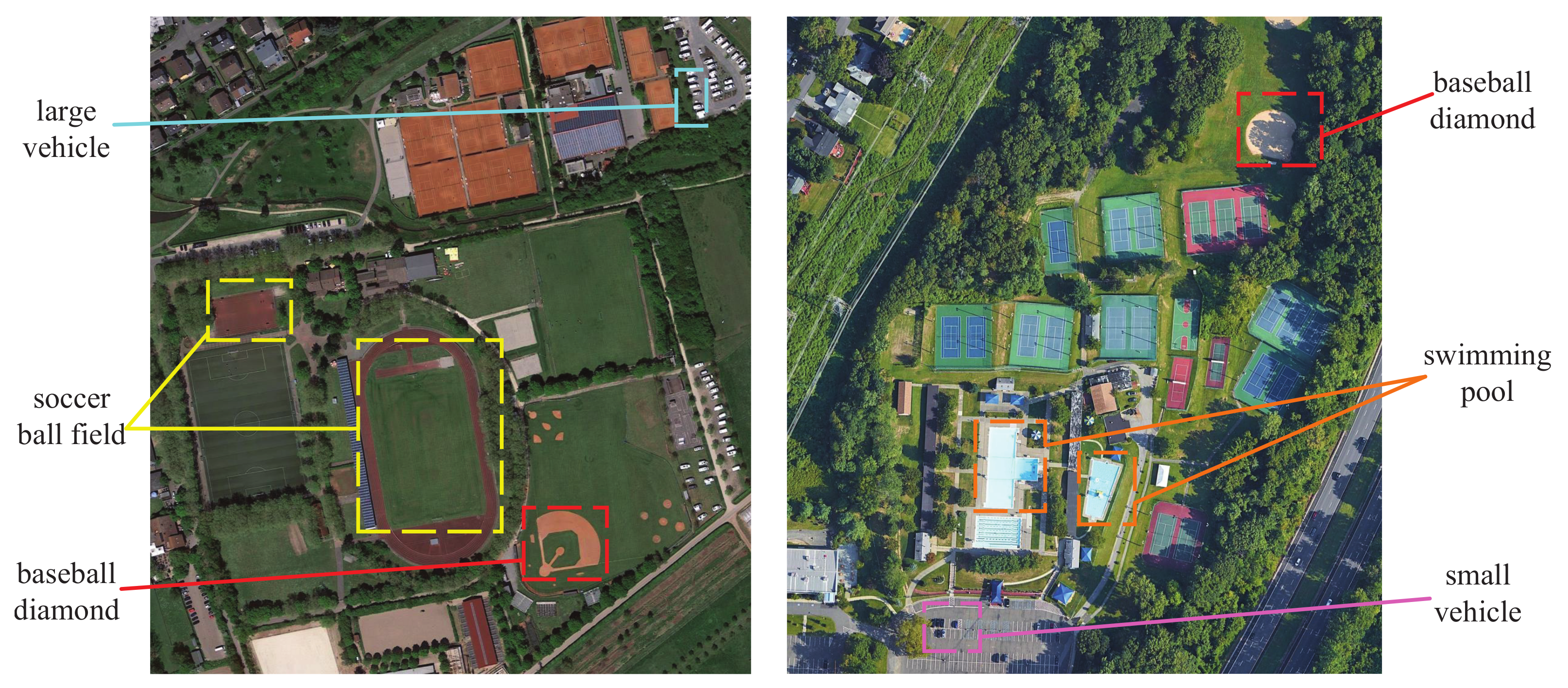
4.1.1. Dataset Description

To demonstrate the semantic segmentation performance of the proposed PGNet on VHR remote sensing images, we conducted extensive experiments on two benchmark datasets: the iSAID dataset [24] (https://captain-whu.github.io/iSAID/dataset.html, accessed on 30 June 2022) and the ISPRS Vaihingen dataset [25] (https://www.isprs.org/education/benchmarks/UrbanSemLab/2d-sem-label-vaihingen.aspx, accessed on 30 June 2022). As shown in

Table 1. The specification of the VHR remote sensing images datasets.

Name	Year	Training	Validation	Test	Class	Metrics
iSAID dataset [24]	2019	1411	937	458	16	$IoU$
ISPRS Vaihingen dataset [25]	2016	11	0	5	6	$IoU$, $F_1$, $OA$

, the iSAID and the ISPRS Vaihingen dataset are two datasets with different characteristics.

(1) The iSAID dataset. The Instance Segmentation in Aerial Images dataset (iSAID) [24] was modified from a large-scale object detection dataset, DOTA [50]. This densely annotated dataset contains 655,451 object instances for 15 categories across 2806 high-resolution images. These categories include planes, ships, storage tanks, harbors, bridges, large vehicles, small vehicles, helicopters, roundabouts, baseball diamonds, tennis courts, basketball courts, ground track fields, soccer ball fields, and swimming pools. The size of the images ranges from 12,029 $\times 5014$ to $455\times 387$. The iSAID training set contains 1411 images, while the validation set contains 458 images, and the test set contains 937 images. However, the test set’s annotations are unavailable, so we used the validation set as the test set in the testing stage, the same as [3,19,51].

(2) The ISPRS Vaihingen dataset. The ISPRS Vaihingen dataset [25] contains 33 VHR remote sensing images collected by advanced airborne sensors, covering a 1.38 km² area of Vaihingen, a relatively small village with many detached buildings and small multi-story buildings. The ground sampling distance (GSD) is about 9 cm, and the average image size is $2494\times 2064$. The ISPRS Vaihingen dataset contains 16 images with manually annotated pixel-by-pixel labels. Each pixel is divided into six most common landcover classes: impervious surfaces, buildings, low vegetation, trees, cars, and clutter/background. The 16 tiles where the ground truth is available were split into a training subset (tile numbers: 1, 3, 5, 7, 13, 17, 21, 23, 26, 30, and 37) and a hold-out subset for evaluation (tile numbers: 11, 15, 28, 32, and 34).

4.1.2. Comparison Methods and Evaluation Metrics

Intending to fully prove the performance of the proposed PGNet for semantic segmentation of VHR remote sensing images, we compared the proposed PGNet with eight SOTA semantic segmentation methods, which are UNet (2015) [46], DeepLabv3 (2017) [23], DeepLabv3+ (2018) [52], the semantic FPN (SFPN) (2019) [47], MACUNet (2022) [20], MAResU-Net (2021) [21], FactSeg (2022) [3], and MANet (2021) [18].

In order to fairly compare with SOTA method on two datasets, we used the widely used evaluation metrics. On the iSAID dataset, we followed the setup of previous works [3,19,51] and used the intersection over union ($IoU$) as the evaluation metric. The $IoU$ is calculated as follows:

$$Io{U}_i=\frac{x_{i,i}}{{\sum }_{i=1}^n{x}_{i,j}+{\sum }_{i=1}^n{x}_{j,i}-x_{i,i}},$$

(16)

$$mIoU=\frac{1}{n}\sum _{i=1}^{n}Io{U}_i,$$

(17)

where $x_{i,j}$ means the number of instances of class i predicted as class j, and n is the number of classes. On the ISPRS Vaihingen dataset, we also followed the setup of previous works [3,18,21,25], calculating the confusion matrices and extracting the overall accuracy ($OA$) and the $F_1$ score of each class to evaluate the semantic segmentation results. The $F_1$ score is a comprehensive evaluation metric of the accuracy and recall and is calculated as shown in Equation (18).

$$F_1=2\times \frac{precision\times recall}{precision+recall},$$

(18)

where $precision=\frac{TP}{TP+FP}$ and $recall=\frac{TP}{TP+FN}$. The $OA$ is the ratio of the number of correctly predicted pixels to the total number of pixels and is calculated as follows:

$$OA=\frac{TP+TN}{P+N}.$$

(19)

4.1.3. Implementation Details

The PGNet is implemented (https://github.com/Fhujinwu/PGNet, accessed on 21 July 2022) in the PyTorch framework [53], trained and tested on a platform with an Intel(R) Xeon(R) Gold 5218 CPU @2.30 GHz, NVIDIA Tesla V100 GPU with CUDA version 10.1. Since the iSAID and the ISPRS Vaihingn dataset are vastly different in terms of image size and data volume, the details of the implemented parameters are generally different, as shown in previous works [3,22]. On the iSAID dataset, we randomly cropped $896\times 896$ patches from the original image and randomly mirrored and rotated them. The widely used SGD optimizer was used with a momentum of 0.9, a weight decay of 0.0001, an initial learning rate of 0.007, and a “poly” scheme with a power of 0.9. The batch size was set to 8, and the network was trained in 70,000 steps. For the test stage, we used the sliding window technique with a window size of $896\times 896$ and a stride count of 512. On the ISPRS Vaihingen dataset, we randomly cropped $512\times 512$ patches from the original image and randomly mirrored and rotated them. The widely used SGD optimizer was used with a momentum of 0.9, a weight decay of 0.0001, an initial learning rate of 0.007, and a “poly” scheme with a power of 0.9. The batch size was set to 4, and the network was trained in 10,000 steps. During the test stage, the sliding window size was set to $512\times 512$, and the number of strides was 256.

4.2. Comparative Experiments and Analysis

We followed the experimental setup in Section 4.1 and conducted extensive experiments on two benchmark datasets, the iSAID and the Vaihingen dataset, to compare the performance of our proposed PGNet and SOTA methods including UNet (2015) [46], DeepLabv3 (2017) [23], DeepLabv3+ (2018) [52], the semantic FPN (SFPN) (2019) [47], MACUNet (2022) [20], MAResU-Net (2021) [21], FactSeg (2022) [3], and MANet (2021) [18].

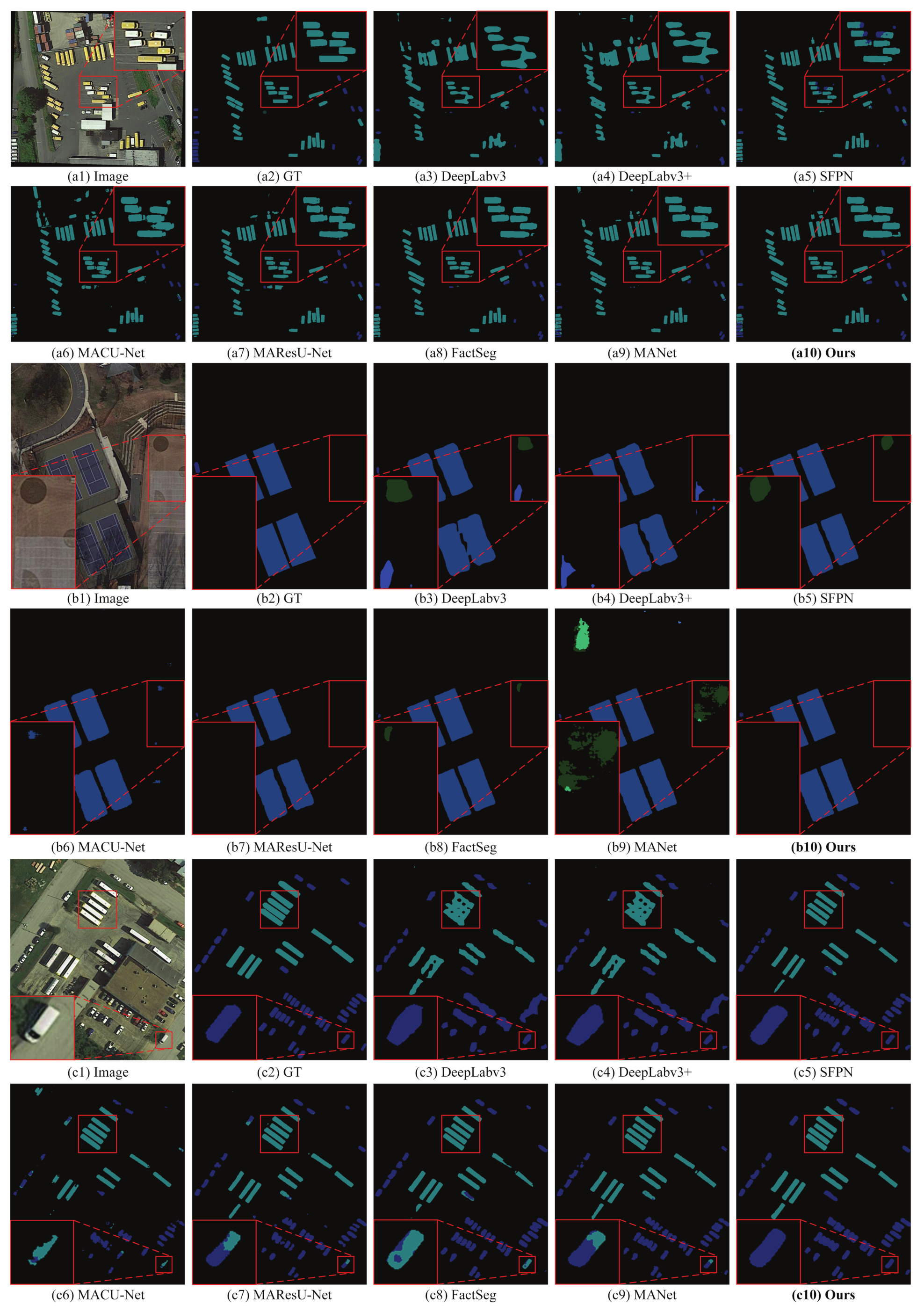
4.2.1. Experiments on the iSAID Dataset

The iSAID dataset is a challenging VHR remote sensing image dataset because of the semantic class diversity and scene complexity. To demonstrate the performance of the proposed PGNet on this challenging VHR remote sensing images dataset, we conducted extensive comparison experiments between PGNet and eight SOTA methods, and the experimental results are shown in

Table 2. The quantitative results of PGNet and SOTA methods on the iSAID dataset. The best results are highlighted in bold, and the second-best is marked in underline. Result form: mean ± standard deviation.

Method	$\mathit{mIoU}(\%)$	$\mathit{IoU}$ per Class (%)																Rank
		BG	Ship	ST	BD	TC	BC	GTF	Bridge	LV	SV	HC	SP	RA	SBF	Plane	Harbor
UNet [46]	35.57 (±5.63)	98.16 (±0.22)	48.10 (±3.81)	0.00 (±0.00)	17.09 (±15.32)	73.20 (±10.19)	8.74 (±8.01)	18.44 (±4.09)	3.66 (±3.22)	51.58 (±3.36)	36.43 (±2.48)	0.00 (±0.00)	32.81 (±5.32)	39.09 (±5.81)	26.53 (±18.45)	69.47 (±7.17)	45.84 (±3.46)	8
DeepLabv3 [23]	59.26 (±0.25)	98.72 (±0.01)	59.78 (±0.31)	52.17 (±1.09)	76.05 (±0.95)	84.64 (±0.12)	60.44 (±0.43)	59.61 (±0.83)	32.45 (±0.55)	54.94 (±0.12)	34.52 (±0.09)	28.55 (±1.44)	44.70 (±0.94)	66.85 (±0.24)	73.93 (±0.68)	75.98 (±0.03)	44.66 (±0.81)	5
DeepLabv3+ [52]	59.45 (±0.07)	98.72 (±0.01)	59.38 (±0.08)	52.56 (±1.05)	77.23 (±0.77)	84.72 (±0.21)	61.11 (±0.75)	59.74(±1.79)	32.65 (±0.29)	54.96 (±0.25)	34.77 (±0.62)	28.70 (±1.92)	44.91 (±0.85)	66.62 (±0.63)	74.28 (±0.20)	76.06 (±0.16)	44.87 (±0.97)	4
SFPN [47]	61.55 (±0.17)	98.85 (±0.01)	64.58 (±0.25)	58.41 (±2.16)	75.19 (±0.89)	86.65 (±0.28)	57.83 (±1.07)	51.51 (±1.18)	33.88 (±0.53)	58.75 (±0.45)	45.21 (±0.07)	30.82 (±1.10)	47.82 (±0.49)	68.65 (±0.28)	72.16 (±0.91)	81.15 (±0.29)	53.31 (±0.21)	3
MACU-Net [20]	31.44 (±0.71)	98.12 (±0.06)	44.53 (±0.49)	0.00 (±0.00)	2.57 (±4.46)	67.57 (±0.87)	0.14 (±0.24)	23.64 (±1.54)	0.00 (±0.00)	47.05 (±0.69)	29.32 (±2.57)	0.00 (±0.00)	26.31 (±8.93)	13.01 (±7.12)	45.57 (±5.75)	64.06 (±1.03)	41.05 (±1.43)	9
MAResU-Net [21]	44.46 (±2.67)	98.66 (±0.03)	59.92 (±1.10)	8.18 (±14.16)	17.14 (±28.69)	84.64 (±1.46)	42.18 (±4.45)	47.14 (±2.42)	3.09 (±4.46)	56.92 (±0.65)	40.01 (±0.77)	0.00 (±0.00)	0.83 (±1.44)	64.28 (±2.06)	61.04 (±2.81)	78.64 (±0.83)	48.73 (±1.78)	7
FactSeg [3]	63.88 (±0.32)	98.91 (±0.01)	68.34 (±0.30)	60.01(±2.48)	77.02 (±0.84)	89.04(±0.29)	57.36 (±1.15)	53.32 (±1.65)	36.62 (±0.82)	61.89 (±0.51)	49.51 (±0.61)	38.45(±0.76)	50.09 (±0.50)	71.39 (±0.82)	71.70 (±0.55)	83.90 (±0.37)	54.53 (±0.75)	2
MANet [18]	58.90 (±1.46)	98.84 (±0.03)	64.29 (±1.15)	50.06 (±3.62)	69.40 (±1.93)	87.67 (±0.18)	56.96 (±1.46)	48.18 (±3.28)	31.33 (±0.93)	59.40 (±0.52)	46.36 (±1.15)	10.44 (±14.64)	45.74 (±2.26)	68.60 (±0.23)	68.15 (±1.40)	81.91 (±0.31)	55.06 (±0.97)	6
Ours	65.37(±0.20)	98.96(±0.02)	70.76(±0.37)	59.74 (±2.57)	77.42(±0.23)	88.56 (±0.09)	65.41(±0.46)	54.32 (±4.40)	37.35(±0.40)	62.35(±0.19)	51.85(±0.35)	38.09 (±0.61)	50.26(±2.94)	73.08(±0.39)	75.53(±0.32)	84.85(±0.12)	57.43(±0.88)	1

The abbreviations are as follows: BG—background, ST—storage tank, BD—baseball diamond, TC—tennis court, BC—basketball court, GTF—ground track field, LV—large vehicle, SV—small vehicle, HC—helicopter, SP—swimming pool, RA—roundabout, SBF—soccer ball field.

. PGNet achieves a score of 65.37% in $mIoU$ and almost the highest $IoU$ score in each class. Specifically, the $mIoU$ score of our PGNet is 1.49% higher than the second-best method, FactSeg, and 3.82% higher than the third-best method, SFPN. In particular, our method achieves SOTA performance on the hard-to-segment semantic classes of “ship”, “bridge” and “soccer ball field”. On the segmentation of “ship” objects, the $IoU$ score of our PGNet is 2.42% higher than the second-best method, Factseg, and 6.18% higher than the third-best method, SFPN. On the segmentation of “bridge” objects, the $IoU$ score of our PGNet is 0.73% higher than the second-best method, FactSeg, and 3.47% higher than the third-best method, SFPN. On the segmentation of “soccer ball field” objects, the $IoU$ score of our PGNet is 1.25% higher than the second-best method, DeepLabv3+, and 1.60% higher than the third-best method, DeepLabv3.

Further highlighting the performance of our PGNet on the semantic segmentation task of VHR remote sensing images, we conducted more detailed visual comparison experiments and provided the corresponding visual comparison maps. The visualization results of PGNet compared to the SOTA methods on the iSAID dataset are shown in Figure 5. We can find three advantages of PGNet compared to SOTA methods. The first one is that PGNet can have high segmentation accuracy on objects with small inter-class variation, such as the “small vehicle” and the “large vehicle” in the third image. The second one is that PGNet can have better segmentation results on objects with large intra-class variation, such as the incorrect segmentation of the “baseball diamond” in the second image. The third is that accurate segmentation is possible on objects of small and varying sizes, such as the “vehicle” in the first image. In conclusion, our proposed PGNet can achieve excellent semantic segmentation performance on the iSAID dataset, a challenging large VHR remote sensing images dataset.

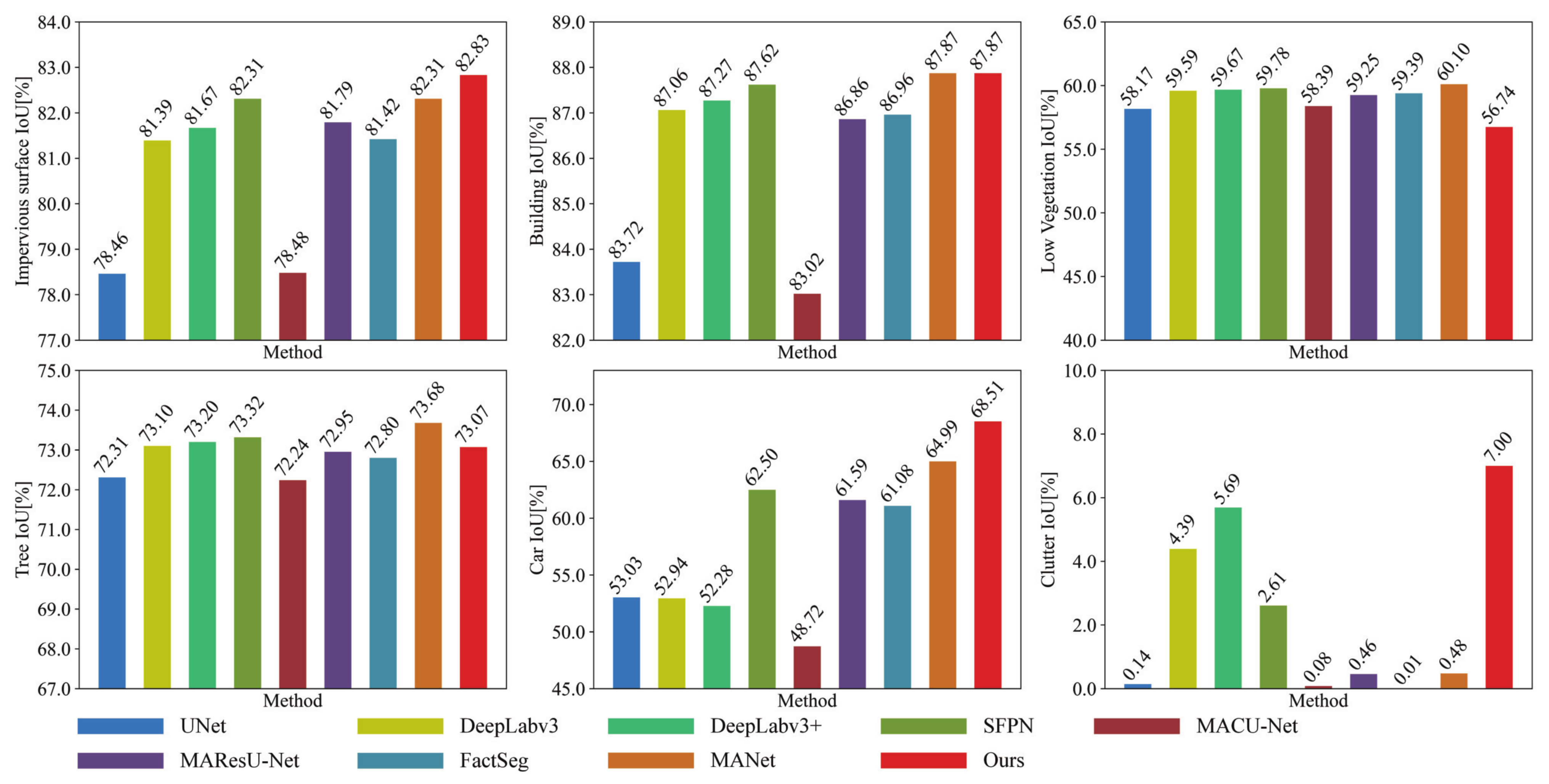
4.2.2. Experiments on the ISPRS Vaihingen Dataset

The ISPRS Vaihingen dataset is a widely used dataset for semantic segmentation of VHR remote sensing images, which is different from the iSAID dataset, which has fewer data and classes. Therefore, we compared the proposed PGNet and SOTA methods on the ISPRS Vaihingen dataset to validate the semantic segmentation performance of PGNet on the VHR remote sensing images dataset with fewer data.

The results of our PGNet compared with SOTA methods on the ISPRS Vaihingen dataset are shown in

Table 3. The quantitative results of PGNet and SOTA methods on the ISPRS Vaihingen dataset.

Method	$\mathit{mIoU}(\%)$	${\mathit{mF}}_1(\%)$	$\mathit{OA}(\%)$	${\mathit{F}}_1$ per Class (%)						Rank
				Impervious Surface	Building	Low Vegetation	Tree	Car	Clutter
UNet [46]	57.63 (±0.36)	67.69 (±0.22)	84.62 (±0.21)	87.93 (±0.38)	91.13 (±0.36)	73.55 (±0.19)	83.92 (±0.27)	69.30 (±0.97)	0.29 (±0.40)	8
DeepLabv3 [23]	59.75 (±0.24)	69.93 (±0.42)	85.96 (±0.12)	89.74 (±0.12)	93.08 (±0.20)	74.67 (±0.30)	84.46 (±0.02)	69.23 (±0.36)	8.38 (±2.46)	7
DeepLabv3+ [52]	59.97 (±0.15)	70.30 (±0.19)	86.07 (±0.09)	89.91 (±0.13)	93.21 (±0.06)	74.74 (±0.22)	84.53 (±0.15)	68.66 (±0.40)	10.76 (±1.08)	6
SFPN [47]	61.21 (±0.42)	70.57 (±0.66)	86.36 (±0.08)	90.29 (±0.07)	93.04 (±0.07)	74.82 (±0.15)	84.60 (±0.10)	76.92 (±0.27)	3.39 (±3.46)	3
MACU-Net [20]	56.82 (±0.21)	66.99 (±0.14)	84.48 (±0.17)	87.94 (±0.32)	90.72 (±0.38)	73.73 (±0.32)	83.88 (±0.18)	65.51 (±1.14)	0.16 (±0.25)	9
MAResU-Net [21]	60.48 (±0.14)	69.81 (±0.23)	85.92 (±0.05)	89.98 (±0.24)	92.97 (±0.25)	74.41 (±0.31)	84.36 (±0.17)	76.23 (±0.80)	0.91 (±1.30)	4
FactSeg [3]	60.27 (±0.51)	69.57 (±0.38)	85.95 (±0.18)	89.76 (±0.23)	93.02 (±0.11)	74.52 (±0.42)	84.25 (±0.10)	75.82 (±1.66)	0.01 (±0.02)	5
MANet [18]	61.57 (±0.08)	70.58 (±0.22)	86.51(±0.01)	90.29 (±0.02)	93.53 (±0.13)	75.07(±0.07)	84.84(±0.05)	78.78 (±0.42)	0.95 (±1.65)	2
Ours	62.67(±0.30)	72.56(±0.32)	86.32 (±0.06)	90.61(±0.12)	93.54(±0.13)	72.39 (±0.28)	84.44 (±0.25)	81.31(±1.10)	13.08(±1.88)	1

and Figure 6. Our proposed PGNet achieves SOTA in the overall segmentation. Specifically, our method outperforms the second-best method, MANet, by 1.10% and the third-best method, SFPN, by 1.46% in the $mIoU$ score. The $m{F}_1$ score of our PGNet is 1.98% higher than the second-best method, MANet, and 1.99% higher than the third-best method, SFPN. As can be observed from Table 3 and Figure 6, our method can also show better results on the “Clutter” objects, a semantic class that is difficult to segment. On the segmentation of “Clutter” objects, the $F_1$ score of our PGNet is 2.32% higher than the second-best method, DeepLabv3+, and 4.70% higher than the third-best method, DeepLabv3, while the $IoU$ score of our PGNet is 1.31% higher than the second-best method, DeepLabv3+, and 2.61% higher than the third-best method, DeepLabv3.

Figure 5. The visualization results of the proposed PGNet and SOTA methods on the iSAID dataset.

Figure 5. The visualization results of the proposed PGNet and SOTA methods on the iSAID dataset.

In addition, we conducted many detailed visual comparison experiments to further confirm the performance of the proposed PGNet for semantic segmentation on ISPRS Vaihingen, a VHR remote sensing image dataset, and provided the corresponding visual comparison maps. The visualization results of our PGNet and SOTA methods are shown in Figure 7. Thanks to our PGM, which effectively transfers global information and long-range dependence to each pyramid-level feature map, PGNet can effectively segment objects with small inter-class variations, such as the “Clutter” and “Building” objects in Figure 7, and objects with large intra-class variations, such as the “Building” objects in Figure 7. Additionally, because our SMCM can effectively collect multi-scale information and generate high-resolution feature maps with high-level semantic information, our PGM can segment objects in small and varying sizes, such as the “Car” objects.

4.3. Ablation Experiments

In this subsection, we evaluated the effectiveness of two key modules of our proposed PGNet, the positioning guidance module (PGM) and the self-multiscale collection module (SMCM). The ablation experiments were trained and tested on the large-scale iSAID and the ISPRS Vaihingen dataset. We conducted extensive ablation experiments using a combination of Res2Net50 [44] and FPN-like structures [47] as the baseline model (Bas.). Specifically, Res2Net50 was used as a feature extractor to obtain pyramid-level features $C_i(i=1,2,3,4)$, and the final output $Out$ was obtained following Equation (20)’s operation.

$$Out=Up(Up(Up(Up\left(C_4\right)+C_3)+C_2)+C_1)$$

(20)

4.3.1. Effect of Positioning Guidance Module

We trained the “Bas. + PGM” model based on the baseline model (Bas.) to evaluate the effectiveness of our proposed PGM. As shown in

Table 4. The results of ablation experiments on the iSAID dataset. The best results are highlighted in bold, and the second-best is marked in underline.

Version	$\mathit{mIoU}(\%)$	$\mathit{IoU}$ per Class (%)
		BG	Ship	ST	BD	TC	BC	GTF	Bridge	LV	SV	HC	SP	RA	SBF	Plane	Harbor
Bas.	63.15	98.90	69.04	54.69	79.77	87.72	63.07	51.93	36.62	61.45	49.36	37.48	45.48	67.01	69.28	83.71	54.95
Bas. + PGM	65.16	98.96	70.29	67.74	78.68	87.80	59.87	58.79	37.58	60.25	50.30	36.69	50.21	70.37	74.82	84.04	56.23
Bas. + PGM + SMCM	65.55	98.98	70.77	58.63	77.54	88.62	64.96	57.70	37.50	62.15	52.19	38.68	50.28	73.06	75.78	84.94	57.07

and

Table 5. The results of ablation experiments on the ISPRS Vaihingen dataset. The best results are highlighted in bold, and the second-best is marked in underline.

Version	$\mathit{mIoU}(\%)$	${\mathit{mF}}_1(\%)$	$\mathit{OA}(\%)$	${\mathit{F}}_1$ per Class (%)
				Impervious Surface	Building	Low Vegetation	Tree	Car	Clutter
Bas.	60.83	69.96	86.25	90.31	93.16	75.08	84.10	77.13	0.00
Bas. + PGM	61.13	70.17	86.23	90.46	93.23	74.83	84.34	78.18	0.09
Bas. + PGM + SMCM	62.88	72.91	86.35	90.57	93.54	72.23	84.52	81.44	15.14

, on the iSAID dataset, the “Bas. + PGM” model increases the $mIoU$ score from 63.15% to 65.16%, a relative increase of 2.01% compared to Bas. Additionally, on the ISPRS Vaihingn dataset, the “Bas. + PGM” model improves the $m{F}_1$ score by 0.48%. This enhancement mainly comes from the fact that the transformer architecture can locate different objects well, and our proposed PGM can effectively transfer the positioning information flow to each pyramid-level feature. The positioning guiding flows contain global context information, which helps to segment objects with large intra-class variations, such as the “swimming pool” and “soccer ball field” in Table 4, improving their $IoU$ scores by 4.73% and 5.54%, respectively. In addition, the positioning guiding flows contain long-range dependence. It achieves good segmentation performance for objects that are camouflaged in the background, e.g., the $IoU$ score of the “plane” in Table 4 is improved by 0.33%. Because the positioning guiding flows is globally informative, this may lead to performance degradation of the method on some small objects, such as the “large vehicles” in Table 4. However, our PGM still provides a significant performance improvement for segmentation.

Figure 7. The visualization results of the proposed PGNet and SOTA methods on the ISPRS Vaihingen dataset.

Figure 7. The visualization results of the proposed PGNet and SOTA methods on the ISPRS Vaihingen dataset.

4.3.2. Effect of Self-Multiscale Collection Module

We trained the “Bas. + PGM + SMCM” model to evaluate the effectiveness of our proposed SMCM. As can be seen in Table 4 and Table 5, the segmentation performance on most of the classes of objects is improved to some degree after adding SMCM. Specifically, the “Bas. + PGM + SMCM” model improves the $mIoU$ score by 0.39% compared to “Bas. + PGM” on the iSAID dataset, while the $m{F}_1$ score is improved by 2.74% on the ISPRS Vaihingn dataset. In addition, the “large vehicle” and “small vehicle”, which are small and highly variable in size in VHR remote sensing images, obtain 1.90% and 1.89% improvement in $IoU$ scores, respectively. This enhancement is made thanks to our proposed SMCM’s ability to obtain high-resolution feature maps with multi-scale and high-level semantic information. The multi-scale information helps our method achieve better segmentation of objects with large-scale variations. At the same time, high-resolution feature maps with high-level semantic information help segment smaller objects. It can effectively compensate for the performance degradation of some small objects such as “large vehicle” due to the use of PGM. Therefore, both the PGM and the SMCM are essential modules.

4.3.3. The Visualization Results of Ablation Experiments

To further demonstrate the effectiveness of our proposed PGM and SMCM, we conducted extensive visualization ablation experiments and provided the corresponding visualization results. As shown in Figure 8, we gradually added our proposed PGM and SMCM on top of Bas. and the semantic segmentation results of VHR remote sensing images were all improved to some degree. For example, the segmentation of the “bridge” in the second row has been improved with the addition of PGM and SMCM. After adding PGM and SMCM progressively, the initially wrong segmentation of “large vehicle” in the third row has been gradually corrected. The results of a large number of ablation experiments fully demonstrate that the two core modules PGM and SMCM in our proposed PGNet help further improve the segmentation outcome of VHR remote sensing images. Specifically, our PGM propagates long-range dependence and global context information to each pyramid-level feature, which helps segment objects with small inter-class and large intra-class variations. The SMCM we designed can obtain high-resolution feature maps with multi-scale and high-level semantic information, which helps segment objects in small and varying sizes in VHR remote sensing images.

4.3.4. Analysis of Different Feature Extractors

Our proposed PGNet is flexible in choosing feature extractors and is not limited to Res2Net50 [44]. Therefore, we conducted ablation experiments using ResNet50 [54] and Res2Net50 as the feature extractor on the iSAID dataset to illustrate the effectiveness of PGNet. As can be seen from

Table 6. The comparison of different feature extractors on the iSAID dataset. The best results are highlighted in bold.

Version	Backbone	$\mathit{mIoU}$	$\Delta$	$\mathit{IoU}$ per Class (%)
				BG	Ship	ST	BD	TC	BC	GTF	Bridge	LV	SV	HC	SP	RA	SBF	Plane	Harbor
Bas.	ResNet50	61.51		98.85	64.29	57.54	76.13	86.33	58.48	50.70	33.31	58.92	45.13	31.48	48.39	68.95	71.24	81.20	53.18
Ours		63.88	+2.37	98.92	67.54	61.30	78.61	87.54	62.01	58.47	34.18	62.40	48.90	33.26	48.52	69.84	72.12	82.77	55.62
Bas.	Res2Net50	63.15		98.90	69.04	54.69	79.77	87.72	63.07	51.93	36.62	61.45	49.36	37.48	45.48	67.01	69.28	83.71	54.95
Ours		65.55	+2.40	98.98	70.77	58.63	77.54	88.62	64.96	57.70	37.50	62.15	52.19	38.68	50.28	73.06	75.78	84.94	57.07

, the proposed PGNet has about 2.40% improvement in $mIoU$ score over Bas. regardless of whether ResNet50 or Res2Net50 is used as the feature extractor. Therefore, it can well demonstrate that PGNet is flexible in choosing feature extractors.

Figure 8. The visualization results of ablation experiments.

Figure 8. The visualization results of ablation experiments.

4.4. Analysis of Methods

On the ISPRS Vaihingn dataset, we further evaluated the PGNet and SOTA methods in $m{F}_1$ score, parameter quantity, and inference time, and the experimental results are shown in

Table 7. The efficiency comparison of PGNet and SOTA on the ISPRS Vaihingen dataset. The best results are highlighted in bold.

Method	${\mathit{mF}}_1$	Parameters (M)	Time (s/Img)
UNet [46]	67.69 ± 0.22	9.85	8.4
DeepLabv3 [23]	69.93 ± 0.42	39.05	11.2
DeepLabv3+ [52]	70.30 ± 0.19	39.05	12.0
SFPN [47]	70.57 ± 0.66	28.48	11.4
MACU-Net [20]	66.99 ± 0.14	5.15	9.8
MAResU-Net [21]	69.81 ± 0.23	26.58	11.6
FactSeg [3]	69.57 ± 0.38	33.45	11.0
MANet [18]	70.58 ± 0.22	35.86	11.2
Ours	72.56 ± 0.32	42.67	12.0

. Although we have more parameters than SOTA methods, it is still within an acceptable range. For example, the proposed PGNet is 1.98% higher in $m{F}_1$ score than the second-best method, MANet, but the number of parameters is only 6.81 M more. In addition, there is no significant difference in inference time between our proposed PGNet and SOTA methods. In conclusion, the proposed PGNet significantly improves the semantic segmentation performance of VHR remote sensing images with the addition of a small number of parameters.

5. Conclusions

In this paper, we proposed a new framework for semantic segmentation of the VHR remote sensing images named Positioning Guidance Network (PGNet), which contains three components, namely, the feature extractor, the positioning guidance module (PGM), and the self-multiscale collection module (SMCM). For the challenge that VHR remote sensing image objects often present large intra-class and small inter-class variations, we designed the PGM to fully leverage the long-range dependence and global contextual information extracted by the transformer architecture and pass them to each pyramid-level feature, thus enhancing the semantic segmentation of VHR remote sensing images. To address the challenge that the objects in VHR remote sensing images are small and of varying sizes, we designed SMCM to effectively extract multi-scale information and generate high-resolution feature maps with high-level semantics, which can help segment these objects.

In addition, we conducted extensive experiments on two challenging datasets, the iSAID and the ISPRS Vaihingen dataset. Through these experiments, we demonstrate that our PGNet can achieve good segmentation results on the semantic segmentation task of VHR remote sensing images. We hope this research can inspire more researchers in this area and deploy practical applications.

References

1. Zhang, C.; Jiang, W.; Zhang, Y.; Wang, W.; Zhao, Q.; Wang, C. Transformer and CNN Hybrid Deep Neural Network for Semantic Segmentation of Very-High-Resolution Remote Sensing Imagery. IEEE Trans. Geosci. Remote Sens. 2022, 60, 4408820. [Google Scholar] [CrossRef]
2. Lazarowska, A. Review of Collision Avoidance and Path Planning Methods for Ships Utilizing Radar Remote Sensing. Remote Sens. 2021, 13, 3265. [Google Scholar] [CrossRef]
3. Ma, A.; Wang, J.; Zhong, Y.; Zheng, Z. FactSeg: Foreground Activation-Driven Small Object Semantic Segmentation in Large-Scale Remote Sensing Imagery. IEEE Trans. Geosci. Remote Sens. 2022, 60, 5606216. [Google Scholar] [CrossRef]
4. Ding, L.; Lin, D.; Lin, S.; Zhang, J.; Cui, X.; Wang, Y.; Tang, H.; Bruzzone, L. Looking outside the window: Wide-context transformer for the semantic segmentation of high-resolution remote sensing images. IEEE Trans. Geosci. Remote Sens. 2022, 60, 4410313. [Google Scholar] [CrossRef]
5. Sahar, L.; Muthukumar, S.; French, S.P. Using aerial imagery and GIS in automated building footprint extraction and shape recognition for earthquake risk assessment of urban inventories. IEEE Trans. Geosci. Remote Sens. 2010, 48, 3511–3520. [Google Scholar] [CrossRef]
6. Tang, X.; Tu, Z.; Wang, Y.; Liu, M.; Li, D.; Fan, X. Automatic Detection of Coseismic Landslides Using a New Transformer Method. Remote Sens. 2022, 14, 2884. [Google Scholar] [CrossRef]
7. Bi, H.; Xu, F.; Wei, Z.; Xue, Y.; Xu, Z. An active deep learning approach for minimally supervised PolSAR image classification. IEEE Trans. Geosci. Remote Sens. 2019, 57, 9378–9395. [Google Scholar] [CrossRef]
8. He, X.; Zhou, Y.; Zhao, J.; Zhang, D.; Yao, R.; Xue, Y. Swin Transformer Embedding UNet for Remote Sensing Image Semantic Segmentation. IEEE Trans. Geosci. Remote Sens. 2022, 60, 4408715. [Google Scholar] [CrossRef]
9. Wang, H.; Chen, X.; Zhang, T.; Xu, Z.; Li, J. CCTNet: Coupled CNN and Transformer Network for Crop Segmentation of Remote Sensing Images. Remote Sens. 2022, 14, 1956. [Google Scholar] [CrossRef]
10. Han, Z.; Hu, W.; Peng, S.; Lin, H.; Zhang, J.; Zhou, J.; Wang, P.; Dian, Y. Detection of Standing Dead Trees after Pine Wilt Disease Outbreak with Airborne Remote Sensing Imagery by Multi-Scale Spatial Attention Deep Learning and Gaussian Kernel Approach. Remote Sens. 2022, 14, 3075. [Google Scholar] [CrossRef]
11. Bi, X.; Hu, J.; Xiao, B.; Li, W.; Gao, X. IEMask R-CNN: Information-enhanced Mask R-CNN. IEEE Trans. Big Data 2022, 1–13. [Google Scholar] [CrossRef]
12. Xiao, B.; Yang, Z.; Qiu, X.; Xiao, J.; Wang, G.; Zeng, W.; Li, W.; Nian, Y.; Chen, W. PAM-DenseNet: A Deep Convolutional Neural Network for Computer-Aided COVID-19 Diagnosis. IEEE Trans. Cybern. 2021, 1–12. [Google Scholar] [CrossRef]
13. Lei, J.; Gu, Y.; Xie, W.; Li, Y.; Du, Q. Boundary Extraction Constrained Siamese Network for Remote Sensing Image Change Detection. IEEE Trans. Geosci. Remote Sens. 2022, 60, 5621613. [Google Scholar] [CrossRef]
14. Bi, X.; Shuai, C.; Liu, B.; Xiao, B.; Li, W.; Gao, X. Privacy-Preserving Color Image Feature Extraction by Quaternion Discrete Orthogonal Moments. IEEE Trans. Inf. Forensics Secur. 2022, 17, 1655–1668. [Google Scholar] [CrossRef]
15. Cheng, J.; Ji, Y.; Liu, H. Segmentation-based PolSAR image classification using visual features: RHLBP and color features. Remote Sens. 2015, 7, 6079–6106. [Google Scholar] [CrossRef]
16. Zhang, X.; Xiao, P.; Song, X.; She, J. Boundary-constrained multi-scale segmentation method for remote sensing images. ISPRS J. Photogramm. Remote Sens. 2013, 78, 15–25. [Google Scholar] [CrossRef]
17. Wang, M.; Dong, Z.; Cheng, Y.; Li, D. Optimal Segmentation of High-Resolution Remote Sensing Image by Combining Superpixels with the Minimum Spanning Tree. IEEE Trans. Geosci. Remote Sens. 2018, 56, 228–238. [Google Scholar] [CrossRef]
18. Li, R.; Zheng, S.; Zhang, C.; Duan, C.; Su, J.; Wang, L.; Atkinson, P.M. Multiattention network for semantic segmentation of fine-resolution remote sensing images. IEEE Trans. Geosci. Remote Sens. 2021, 60, 5607713. [Google Scholar] [CrossRef]
19. Zheng, Z.; Zhong, Y.; Wang, J.; Ma, A. Foreground-aware relation network for geospatial object segmentation in high spatial resolution remote sensing imagery. In Proceedings of the IEEE/CVF Conference on Computer Vision and Pattern Recognition, Seattle, WA, USA, 13–19 June 2020; pp. 4096–4105. [Google Scholar]
20. Li, R.; Duan, C.; Zheng, S.; Zhang, C.; Atkinson, P.M. MACU-Net for Semantic Segmentation of Fine-Resolution Remotely Sensed Images. IEEE Geosci. Remote Sens. Lett. 2022, 19, 8007205. [Google Scholar] [CrossRef]
21. Li, R.; Zheng, S.; Duan, C.; Su, J.; Zhang, C. Multistage attention ResU-Net for semantic segmentation of fine-resolution remote sensing images. IEEE Geosci. Remote Sens. Lett. 2021, 19, 8009205. [Google Scholar] [CrossRef]
22. Chen, F.; Liu, H.; Zeng, Z.; Zhou, X.; Tan, X. BES-Net: Boundary Enhancing Semantic Context Network for High-Resolution Image Semantic Segmentation. Remote Sens. 2022, 14, 1638. [Google Scholar] [CrossRef]
23. Chen, L.C.; Papandreou, G.; Kokkinos, I.; Murphy, K.; Yuille, A.L. Deeplab: Semantic image segmentation with deep convolutional nets, atrous convolution, and fully connected crfs. IEEE Trans. Pattern Anal. Mach. Intell. 2017, 40, 834–848. [Google Scholar] [CrossRef] [PubMed]
24. Waqas Zamir, S.; Arora, A.; Gupta, A.; Khan, S.; Sun, G.; Shahbaz Khan, F.; Zhu, F.; Shao, L.; Xia, G.S.; Bai, X. iSAID: A Large-scale Dataset for Instance Segmentation in Aerial Images. In Proceedings of the IEEE Conference on Computer Vision and Pattern Recognition Workshops, Long Beach, CA, USA, 16–17 June 2019; pp. 28–37. [Google Scholar]
25. Marmanis, D.; Wegner, J.D.; Galliani, S.; Schindler, K.; Datcu, M.; Stilla, U. Semantic segmentation of aerial images with an ensemble of CNSS. ISPRS Ann. Photogramm. Remote Sens. Spat. Inf. Sci. 2016, 3, 473–480. [Google Scholar] [CrossRef]
26. Wang, G.; Ren, P. Hyperspectral image classification with feature-oriented adversarial active learning. Remote Sens. 2020, 12, 3879. [Google Scholar] [CrossRef]
27. Cheng, G.; Yang, C.; Yao, X.; Guo, L.; Han, J. When Deep Learning Meets Metric Learning: Remote Sensing Image Scene Classification via Learning Discriminative CNNs. IEEE Trans. Geosci. Remote Sens. 2018, 56, 2811–2821. [Google Scholar] [CrossRef]
28. Cui, B.; Chen, X.; Lu, Y. Semantic segmentation of remote sensing images using transfer learning and deep convolutional neural network with dense connection. IEEE Access 2020, 8, 116744–116755. [Google Scholar] [CrossRef]
29. Stan, S.; Rostami, M. Unsupervised model adaptation for continual semantic segmentation. In Proceedings of the AAAI Conference on Artificial Intelligence, Virtual, 2–9 February 2021; Volume 35, pp. 2593–2601. [Google Scholar]
30. Bosilj, P.; Aptoula, E.; Duckett, T.; Cielniak, G. Transfer learning between crop types for semantic segmentation of crops versus weeds in precision agriculture. J. Field Robot. 2020, 37, 7–19. [Google Scholar] [CrossRef]
31. Pan, F.; Shin, I.; Rameau, F.; Lee, S.; Kweon, I.S. Unsupervised intra-domain adaptation for semantic segmentation through self-supervision. In Proceedings of the IEEE/CVF Conference on Computer Vision and Pattern Recognition, Seattle, WA, USA, 13–19 June 2020; pp. 3764–3773. [Google Scholar]
32. Xu, Q.; Ma, Y.; Wu, J.; Long, C.; Huang, X. Cdada: A curriculum domain adaptation for nighttime semantic segmentation. In Proceedings of the IEEE/CVF International Conference on Computer Vision, Montreal, QC, Canada, 11–17 October 2021; pp. 2962–2971. [Google Scholar]
33. Diakogiannis, F.I.; Waldner, F.; Caccetta, P.; Wu, C. ResUNet-a: A deep learning framework for semantic segmentation of remotely sensed data. ISPRS J. Photogramm. Remote Sens. 2020, 162, 94–114. [Google Scholar] [CrossRef]
34. Vaswani, A.; Shazeer, N.; Parmar, N.; Uszkoreit, J.; Jones, L.; Gomez, A.N.; Kaiser, Ł.; Polosukhin, I. Attention is all you need. Adv. Neural Inf. Process. Syst. 2017, 30. [Google Scholar]
35. Devlin, J.; Chang, M.W.; Lee, K.; Toutanova, K. Bert: Pre-training of deep bidirectional transformers for language understanding. arXiv 2018, arXiv:1810.04805. [Google Scholar]
36. Dosovitskiy, A.; Beyer, L.; Kolesnikov, A.; Weissenborn, D.; Zhai, X.; Unterthiner, T.; Dehghani, M.; Minderer, M.; Heigold, G.; Gelly, S.; et al. An Image is Worth 16x16 Words: Transformers for Image Recognition at Scale. In Proceedings of the International Conference on Learning Representations, Addis Ababa, Ethiopia, 26–30 April 2020. [Google Scholar]
37. Xie, E.; Wang, W.; Yu, Z.; Anandkumar, A.; Alvarez, J.M.; Luo, P. SegFormer: Simple and efficient design for semantic segmentation with transformers. Adv. Neural Inf. Process. Syst. 2021, 34, 12077–12090. [Google Scholar]
38. Ke, L.; Danelljan, M.; Li, X.; Tai, Y.W.; Tang, C.K.; Yu, F. Mask Transfiner for High-Quality Instance Segmentation. In Proceedings of the IEEE/CVF Conference on Computer Vision and Pattern Recognition, New Orleans, LA, USA, 19–20 June 2022; pp. 4412–4421. [Google Scholar]
39. Wang, W.; Xie, E.; Li, X.; Fan, D.P.; Song, K.; Liang, D.; Lu, T.; Luo, P.; Shao, L. Pyramid Vision Transformer: A Versatile Backbone for Dense Prediction Without Convolutions. In Proceedings of the IEEE/CVF International Conference on Computer Vision (ICCV), Montreal, BC, Canada, 11–17 October 2021; pp. 568–578. [Google Scholar]
40. Liu, Z.; Lin, Y.; Cao, Y.; Hu, H.; Wei, Y.; Zhang, Z.; Lin, S.; Guo, B. Swin Transformer: Hierarchical Vision Transformer Using Shifted Windows. In Proceedings of the IEEE/CVF International Conference on Computer Vision (ICCV), Montreal, BC, Canada, 11–17 October 2021; pp. 10012–10022. [Google Scholar]
41. Mei, H.; Ji, G.P.; Wei, Z.; Yang, X.; Wei, X.; Fan, D.P. Camouflaged object segmentation with distraction mining. In Proceedings of the IEEE/CVF Conference on Computer Vision and Pattern Recognition, Virtual, 19–25 June 2021; pp. 8772–8781. [Google Scholar]
42. Liu, J.J.; Hou, Q.; Liu, Z.A.; Cheng, M.M. Poolnet+: Exploring the potential of pooling for salient object detection. IEEE Trans. Pattern Anal. Mach. Intell. 2022. [Google Scholar] [CrossRef]
43. Wang, D.; Zhang, J.; Du, B.; Xia, G.S.; Tao, D. An Empirical Study of Remote Sensing Pretraining. IEEE Trans. Geosci. Remote Sens. 2022. [Google Scholar] [CrossRef]
44. Gao, S.H.; Cheng, M.M.; Zhao, K.; Zhang, X.Y.; Yang, M.H.; Torr, P. Res2net: A new multi-scale backbone architecture. IEEE Trans. Pattern Anal. Mach. Intell. 2019, 43, 652–662. [Google Scholar] [CrossRef] [Green Version]
45. Hendrycks, D.; Gimpel, K. Gaussian error linear units (gelus). arXiv 2016, arXiv:1606.08415. [Google Scholar]
46. Ronneberger, O.; Fischer, P.; Brox, T. U-net: Convolutional networks for biomedical image segmentation. In Proceedings of the International Conference on Medical Image Computing and Computer-Assisted Intervention, Munich, Germany, 5–9 October 2015; Springer: Berlin/Heidelberg, Germany, 2015; pp. 234–241. [Google Scholar]
47. Kirillov, A.; Girshick, R.; He, K.; Dollár, P. Panoptic feature pyramid networks. In Proceedings of the IEEE/CVF Conference on Computer Vision and Pattern Recognition, Long Beach, CA, USA, 15–20 June 2019; pp. 6399–6408. [Google Scholar]
48. Zhao, H.; Shi, J.; Qi, X.; Wang, X.; Jia, J. Pyramid scene parsing network. In Proceedings of the IEEE Conference on Computer Vision and Pattern Recognition, Honolulu, HI, USA, 21–26 July 2017; pp. 2881–2890. [Google Scholar]
49. Pang, Y.; Zhao, X.; Xiang, T.Z.; Zhang, L.; Lu, H. Zoom in and Out: A Mixed-Scale Triplet Network for Camouflaged Object Detection. In Proceedings of the IEEE/CVF Conference on Computer Vision and Pattern Recognition, New Orleans, LA, USA, 21 June 2022; pp. 2160–2170. [Google Scholar]
50. Xia, G.S.; Bai, X.; Ding, J.; Zhu, Z.; Belongie, S.; Luo, J.; Datcu, M.; Pelillo, M.; Zhang, L. DOTA: A large-scale dataset for object detection in aerial images. In Proceedings of the IEEE Conference on Computer Vision and Pattern Recognition, Salt Lake City, UT, USA, 18–23 June 2018; pp. 3974–3983. [Google Scholar]
51. Li, X.; He, H.; Li, X.; Li, D.; Cheng, G.; Shi, J.; Weng, L.; Tong, Y.; Lin, Z. PointFlow: Flowing semantics through points for aerial image segmentation. In Proceedings of the IEEE/CVF Conference on Computer Vision and Pattern Recognition, Nashville, TN, USA, 20–25 June 2021; pp. 4217–4226. [Google Scholar]
52. Chen, L.C.; Zhu, Y.; Papandreou, G.; Schroff, F.; Adam, H. Encoder-decoder with atrous separable convolution for semantic image segmentation. In Proceedings of the European Conference on Computer Vision (ECCV), Munich, Germany, 8–14 September 2018; pp. 801–818. [Google Scholar]
53. Paszke, A.; Gross, S.; Chintala, S.; Chanan, G.; Yang, E.; DeVito, Z.; Lin, Z.; Desmaison, A.; Antiga, L.; Lerer, A. Automatic Differentiation in Pytorch. In Proceedings of the 31st Conference on Neural Information Processing Systems (NIPS 2017), Long Beach, CA, USA, 4–9 December 2017. [Google Scholar]
54. He, K.; Zhang, X.; Ren, S.; Sun, J. Deep residual learning for image recognition. In Proceedings of the IEEE Conference on Computer Vision and Pattern Recognition, Honolulu, HI, USA, 21–26 July 2016; pp. 770–778. [Google Scholar]
Figure 1. The challenges of semantic segmentation of very-high-resolution remote sensing images.
Remotesensing 14 04219 g001
Figure 2. The framework of the proposed PGNet, which consists of a Res2Net backbone, a positioning guidance module (PGM) and three self-multiscale collection modules (SMCM). T means transformer block and S means SMCM.
Remotesensing 14 04219 g002
Figure 3. The transformer layer (based on the mix transformer [37]) in the positioning guide module.
Remotesensing 14 04219 g003
Figure 4. The architecture of the self-multiscale collection module.
Remotesensing 14 04219 g004
Figure 6. The comparison of the proposed PGNet and SOTA methods on the ISPRS Vaihingen dataset.
Remotesensing 14 04219 g006