Abstract
The effect of the number and configuration of participating stations on lightning location outside the network is herein studied by evaluating the deviation distance between the reference location and the locations determined by the ToA technique, using recorded data from the location network in Fujian. It was found that the deviation distance decreases with the increase of number of stations, changing from 0.07 to 424.7 km with an average of 35 km for five stations while being 0.03~21.6 km and 2.2 km, respectively, for eight stations. The spatial distribution of those locations outside the network seems to be on a straight line. When the number of stations was five, the station linear configuration led to a narrow and long intersection region, resulting in a large deviation distance. The more dispersed distribution of stations leads to the minimum deviation distance. The percentage of deviation distance less than specific location accuracy (LA) can provide references on network design. 7 stations are sufficient to locate the lightning near and inside the network. 8–9 stations are necessary for an LA of 1 km when the lightning is 200 to 300 km away from the center of the network. The network is not suitable for locating the lightning from each station more than 400 km on average.
1. Introduction
Lightning discharges produce wideband electromagnetic radiation, mainly focused on the frequency band from 1 Hz to 300 MHz [1]. Thus, according to different frequency bands of lightning radiation, specific sensors are designed to detect the electromagnetic signals and then these signals received from multiple sensors are time-synchronized by the high precision GPS (Global Positioning System). Using these synchronous signals, different location algorithms are applied to determine the location and occurrence time of lightning discharge. This is a brief description of the operation of the lightning location systems (LLSs).
Many LLSs have been developed and deployed in different countries and regions since the 1980s, mainly divided into very low frequency (VLF), low frequency (LF), LLS and very high frequency (VHF) LLS depending on the detection frequency band. Due to the strong energy and low attenuation, the electromagnetic signal in the VLF/LF band is suitable for large-scale lightning activity monitoring, generally used to locate the return strokes, track the thunderstorm and forecast and warn of severe convective weather [2,3,4,5,6,7,8,9,10,11,12,13,14]. Due to abundant radiation pulses in the VHF band, the lightning electromagnetic signal is used to study the intracloud process of lightning activity, such as the initial breakdown processes (IBP), initial stepped leaders, and a map of the fine structure of lightning channel [15,16,17,18,19].
Since the last century, the regional and worldwide LLSs are developed based on the VLF/LF signal, especially in the commercial operation, such as the National Lightning Detection Network (NLDN) in the United States with the location accuracy within 500 m and the 90% detection efficiency of cloud-ground (CG) discharges [2,3] and the Los Alamos Sferic Array (LASA) with the capability to retrieve 3D positions for VLF/LF sources [4,5] in the United States, the Lightning detection network (LINET) with high accuracy (150 m) total lightning location with separated CG and intracloud (IC) events in Europe [6,7] and the European Cooperation for Lightning Detection (EUCLID) network with high quality lightning data throughout Europe in terms of its location accuracy (LA) and detection efficiency (DE) [9]. In addition to these commercial LLSs, LLSs operating in VHF frequencies have emerged in recent decades, such as Lightning Detection and Ranging (LDAR) [15], Lightning Mapping Array (LMA) [16] and broadband interferometers [17,18,19]. Recently, VLF/LF 3D lightning location networks have been demonstrated to study the intracloud process and describe the detailed development of the lightning channel [20,21,22,23].
In recent years, lightning and thunderstorm detection techniques have been rapidly developed in many regions of Asia. The Broadband Observation Network for Lightning and Thunderstorm positioning system (BOLT) and the Fast Antenna Lightning Mapping Array (FALMA) were deployed in Japan to study the initiation of IC events following a narrow bipolar event (NBE) and reconstruct the 3D lightning channel [24,25,26]. In China, the LLSs have been in operation since their development in the 1980s and have been installed in many areas throughout the country for commercial operation. Their data have been widely used by meteorological organizations [27] and power electric companies [28]. Besides, different research institutions have developed their own LLSs for scientific purposes, such as the Beijing Lightning Network (BLNET) with three kinds of sensors in VLF/LF and VHF domains designed for thunderstorm monitoring and lightning physics research [29,30], the Low-frequency E-field Detection Array (LFEDA) in Guangzhou for 3D LF location of total lightning [31], the Jianghuai Area Sferic Array (JASA) in Anhui province [32,33] for investigating the fluctuation of ionospheric D layer and a 3D VLF/LF lightning location network deployed in north China mapping the development of CG and IG events [34].
These LLS were developed and have been under stable operation for many years. They have diverse baselines, effective coverage, different bandwidth of sensors and different installation environments. The lightning location can be affected by these factors [35,36,37] and the relief of earth surface orography [38,39,40,41]. In addition, the number and configuration of sensors also influence the lightning location. The relevant studies are mostly focused on the Monte Carlo simulation to estimate the location error and to further evaluate network performance [5,29,31,34,42]. They always pay attention to the lightning inside the network and improve the location accuracy by updating the network but neglect the location accuracy for those lightning outside the network.
Various thunderstorm activities occur in the southeast of China every year. This provides an opportunity to track and monitor the lightning activities in the ocean and on the coast. In order to research the effect of number and configuration of participating stations on the quality of the lightning location outside the network, we established a regional lightning detection and location network in Fujian, China. Two types of sensors operating in the VLF/LF frequency band were designed, and six cases detected by the network in 2021 summer from different directions were chosen. First, the validation of the reference location was performed. Then, the deviation distance between the reference location and the locations for different numbers and configuration of participating stations was studied in the form of boxplots. Finally, the configuration of stations under the maximum and minimum deviation distance were shown when the number of participating stations was five.
2. Data and Method
2.1. The Lightning Detection and Location Network
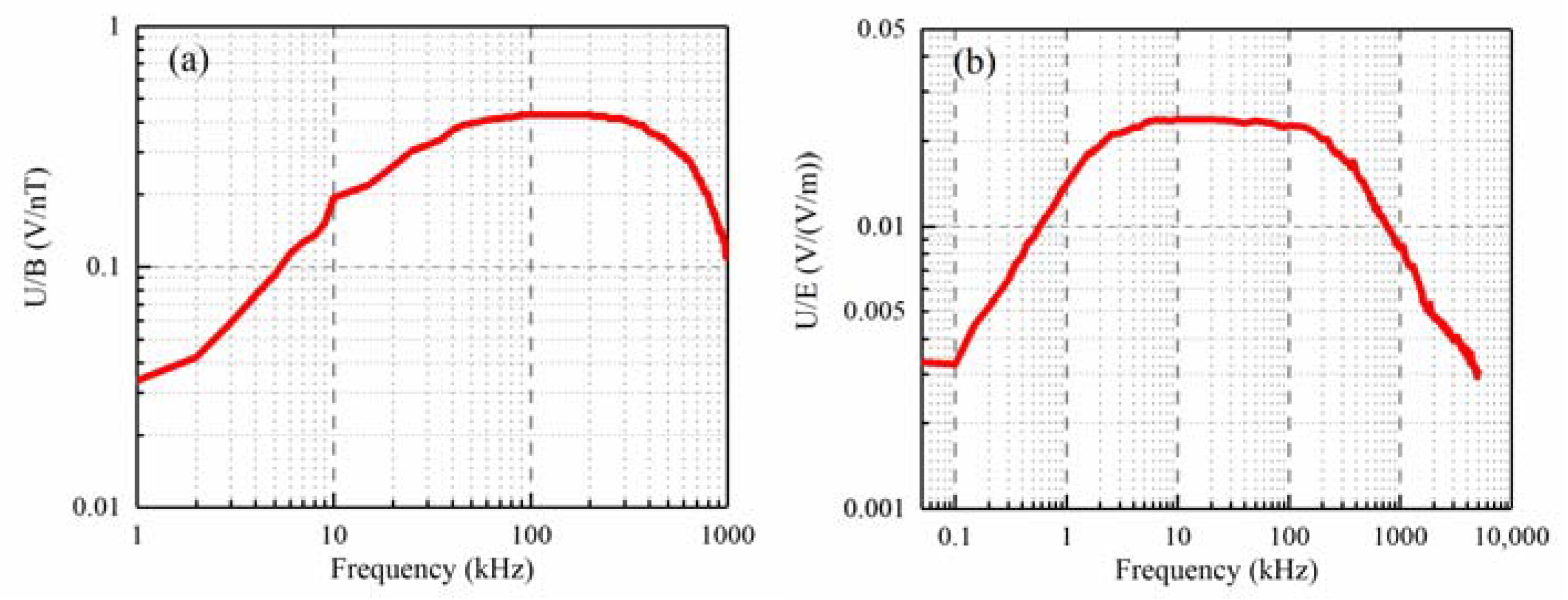
In this paper, a regional lightning detection and location network established in Fujian Province, China since 2021 was employed to detect lightning activity in southeastern China. The network consisted of 10 observation stations, covering an area of about 200 km in the east–west extension and 150 km in north–south extension. Each station was equipped with two orthogonal magnetic field antennas, a signal acquisition system and a GPS receiver. In addition, five stations were equipped with fast electric field antennas. The bandwidth of these two kinds of antennas is from 10 kHz to 500 kHz and 1 kHz to 400 kHz, respectively (see Figure 1). Owing to the relative flat frequency response of fast antennae, from the aspect of waveform, it is beneficial to identify whether the recorded data satisfies the typical lightning return stroke. If the electromagnetic field signal strength exceeded the threshold, it was recorded continuously with a sampling rate of 0.25 MHz, and the recording length is 1 s with the pre-trigger time of 250 ms. All stations were synchronized by GPS with an accuracy of 50 ns.

Figure 1.
The frequency response curve of (a) magnetic field antennas and (b) fast electric field antennas.
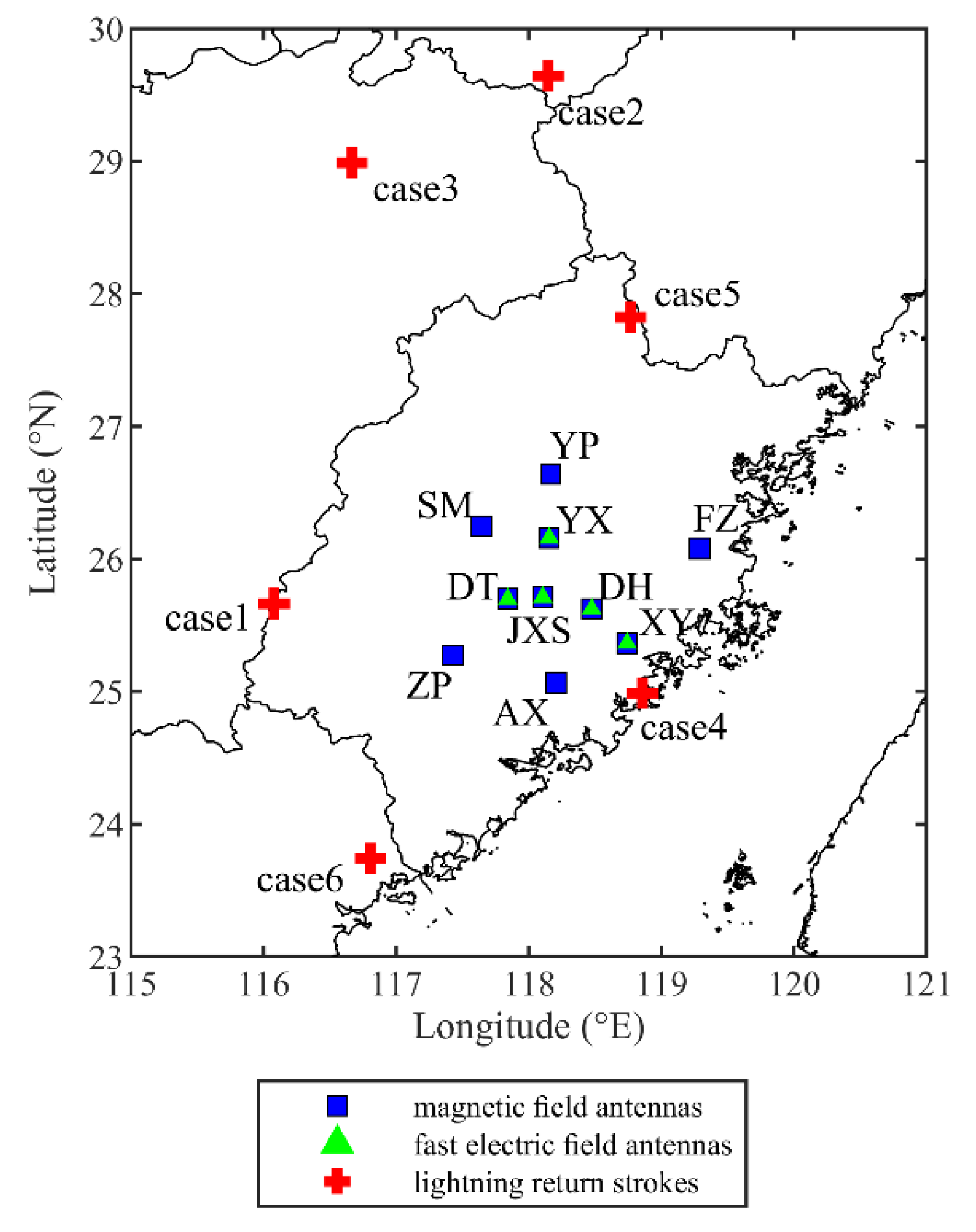
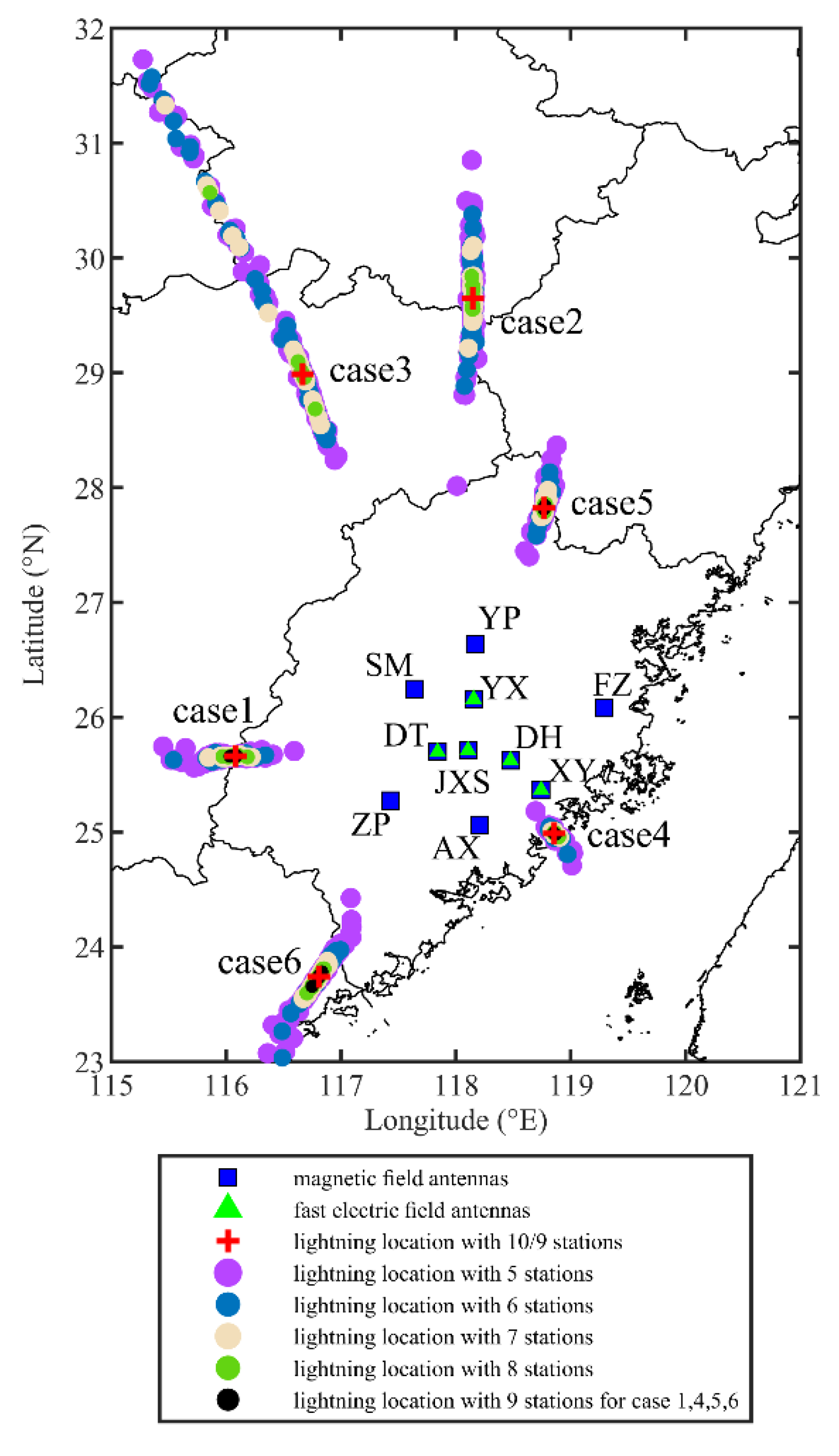
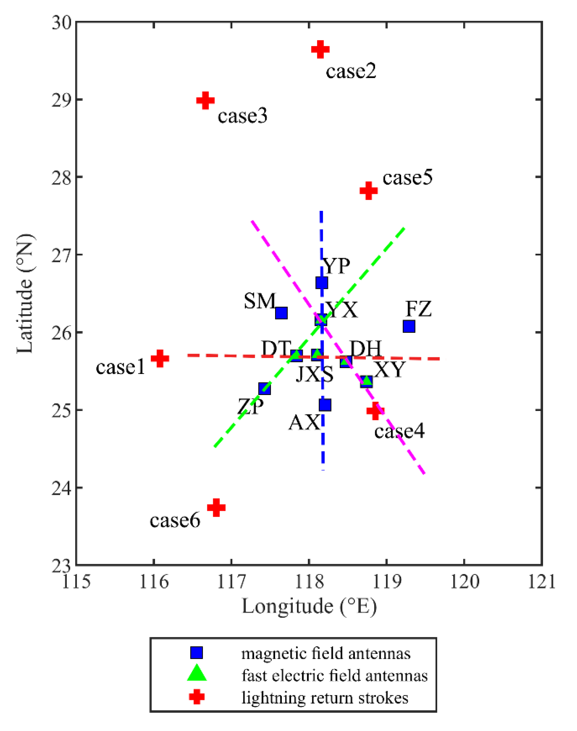
The lightning detection and location network was under stable operation during the summer of 2021. Figure 2 shows the sensor locations within the lightning location network in Fujian Province. Other stations were installed below an elevation of 250 m, except JXS (1667 m) and DH (1654 m) stations. In order to analyze the effect of number and configuration of participating stations on the quality of the lightning location outside the network, six cases from different directions were chosen. The red crosses mark the six cases whose position is estimated by using the ToA technique with the time corresponding to the peak field, using 10 stations’ (9 stations for case 2 and case 3) simultaneous waveforms data. The distances of the six cases to each station are about 220 km, 430 km, 400 km, 120 km, 240 km and 270 km on average, respectively.
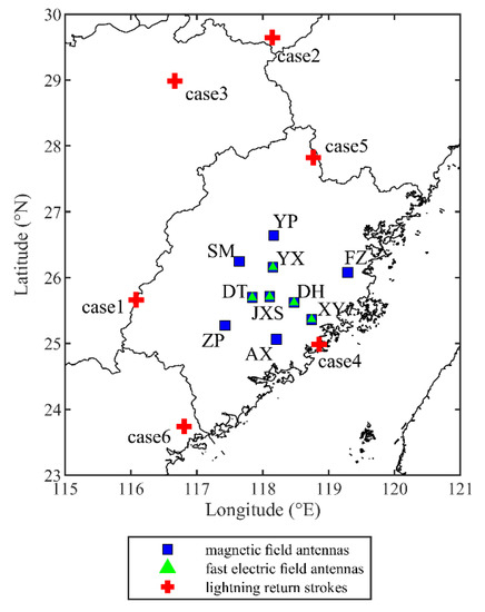
Figure 2.
Sensor locations within the lightning locating network in Fujian Province. The blue squares mark the magnetic field antennas. The green tringles mark the fast electric field antennas. The red crosses mark the lightning return strokes (case 1 to case 6) whose position is estimated by using 10 stations (9 stations for case 2 and case 3) simultaneous waveforms data.
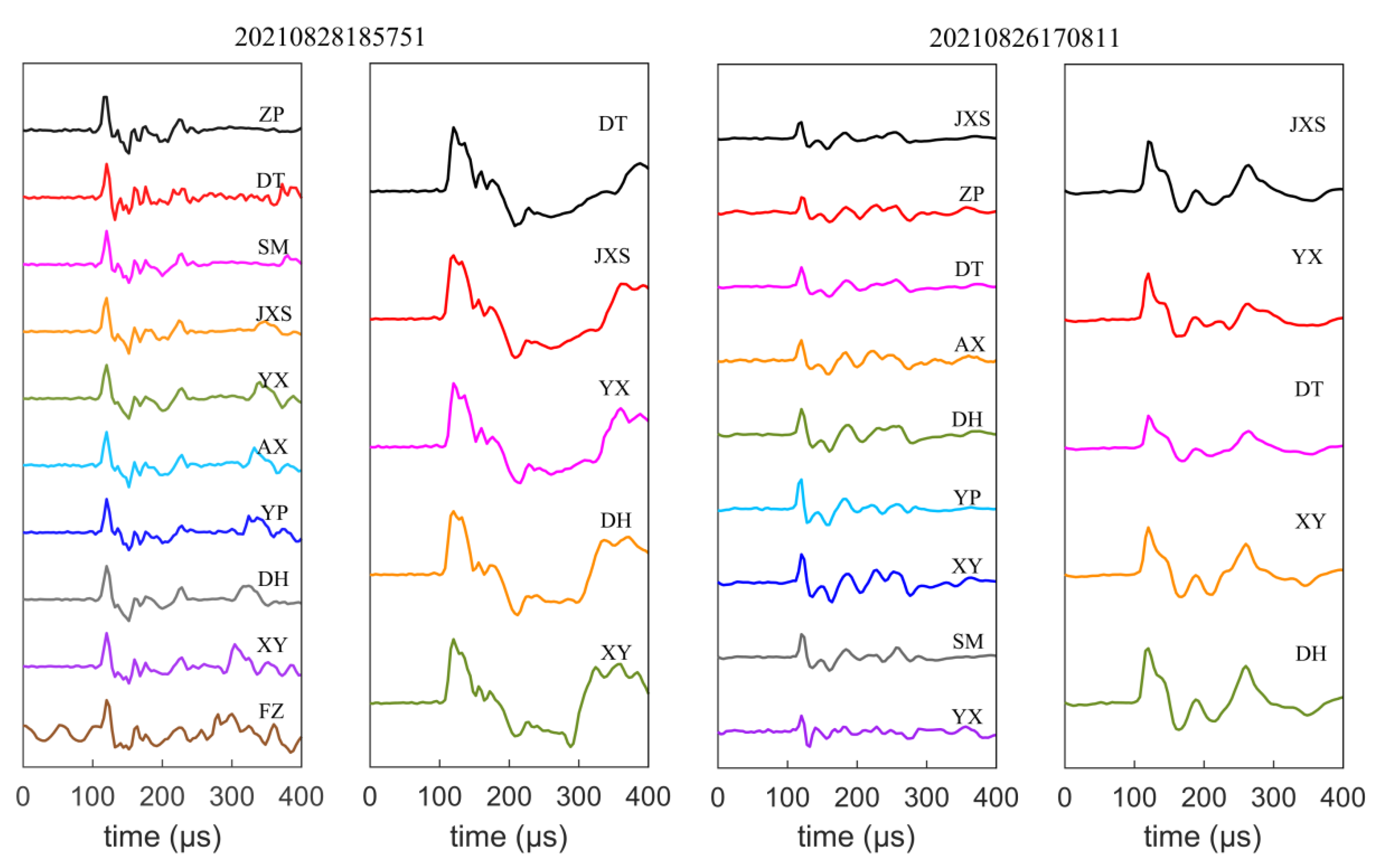
Figure 3 shows the recorded waveforms of lightning return strokes corresponding to the six cases in Figure 2. The left part in the subgraph shows the magnetic field synchronous waveform which was involved in lightning location. The right part is the electric field waveform of the same return stroke, which conforms to the typical return stroke waveform of a fast rise and slow fall. Peak times of the waveforms are aligned to display complete and detailed waveforms. Note that the number of synchronous magnetic field antennas is nine in case 2 and case 3 because of the further distance, while in other cases the number of synchronous antennas is ten.

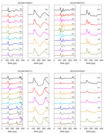
Figure 3.
The recorded synchronous waveforms of lightning return strokes corresponding to six cases in Figure 2. The left part in subgraph shows the magnetic field waveform. The right part is the electric field waveform of the same case.
2.2. Lightning Location Algorithm
The ToA technique is applied to determine the lightning position by using the arrival time differences between observation sites. A lightning electromagnetic signal arriving at each observation site satisfies the following equation:
where, (x, y, z, t) are the lightning coordinates and time, (xi, yi, zi) are the geographic position of ith observation site, ti is the arrival time of the signal at ith observation site (i = 1, 2, …, N, where N is the number of observation sites) and c is the speed of light.
The arrival time of the lightning electromagnetic signal is used to solve the nonlinear equations consisting of N equations in the form of Equation (1). Then, the lightning stroke position (x, y, z) can be estimated by the ToA technique. We used the Chan algorithm [43] to produce the initial guess of the equations and applied the Levenberg–Marquardt method to minimize the goodness-of-fit parameter χ2 [29]:
where and are the observed and fitted arrival time of the ith observation site, respectively; σ2 is the typical timing error; N − 4 is the degree of freedom; N is the number of observation sites.
In this paper, the time corresponding to the peak field and 10% threshold of the peak field were used to determine the arrival time of magnetic field waveform, marked as tp and t10. The time corresponding to 10% threshold of the peak field proposed by Schulz [44] can be expressed as:
where Bp is the peak value of magnetic field waveform and tp is the corresponding time. The threshold BT is set to 10% of Bp and tT is the corresponding time.
Three methods of arrival time differences between the pair of stations are used to estimate the lightning location. Using the time corresponding to the peak field (tp) to compute the arrival time differences was marked as Tp, the 10% threshold of the peak field (t10) was marked as T10. Besides, the waveform cross-correlation can also be applied to the arrival time differences, marked as Tcorr [23].
3. Results
In order to analyze the effect of number and configuration of participating stations on the quality of the lightning location outside the network, six cases from different directions were chosen. The location with the maximum number of synchronization stations was regarded as the reference location of each case. For case 2 and 3, the reference location is the location determined by nine synchronization stations, while in other cases it is determined by ten synchronization stations. The deviation distance between the reference location and the location under different number and configuration of stations can be used to evaluate the impact of these two factors.
The procedures of analysis were as follows. First, the reference location was validated by the tight intersection region consisting of all hyperbolas and by the close correlation with the low cloud top temperature region. Then, the locations under different numbers and different combinations of participating stations were obtained, using the ToA technique with three methods of arrival time differences. After that, the chi-square test was performed to eliminate time gross error, and only the locations which passed the test can be compared with the reference location in the form of boxplots. Finally, for the six cases outside the network, the configuration of stations under the maximum and minimum deviation distance was shown in detail, respectively, when the number of participating stations was five.
3.1. The Validation of Reference Location
Since the exact lightning return strokes positions are unavailable, the locations with the maximum number of synchronization stations were regarded as the reference location to evaluate the deviation distance in the following text.
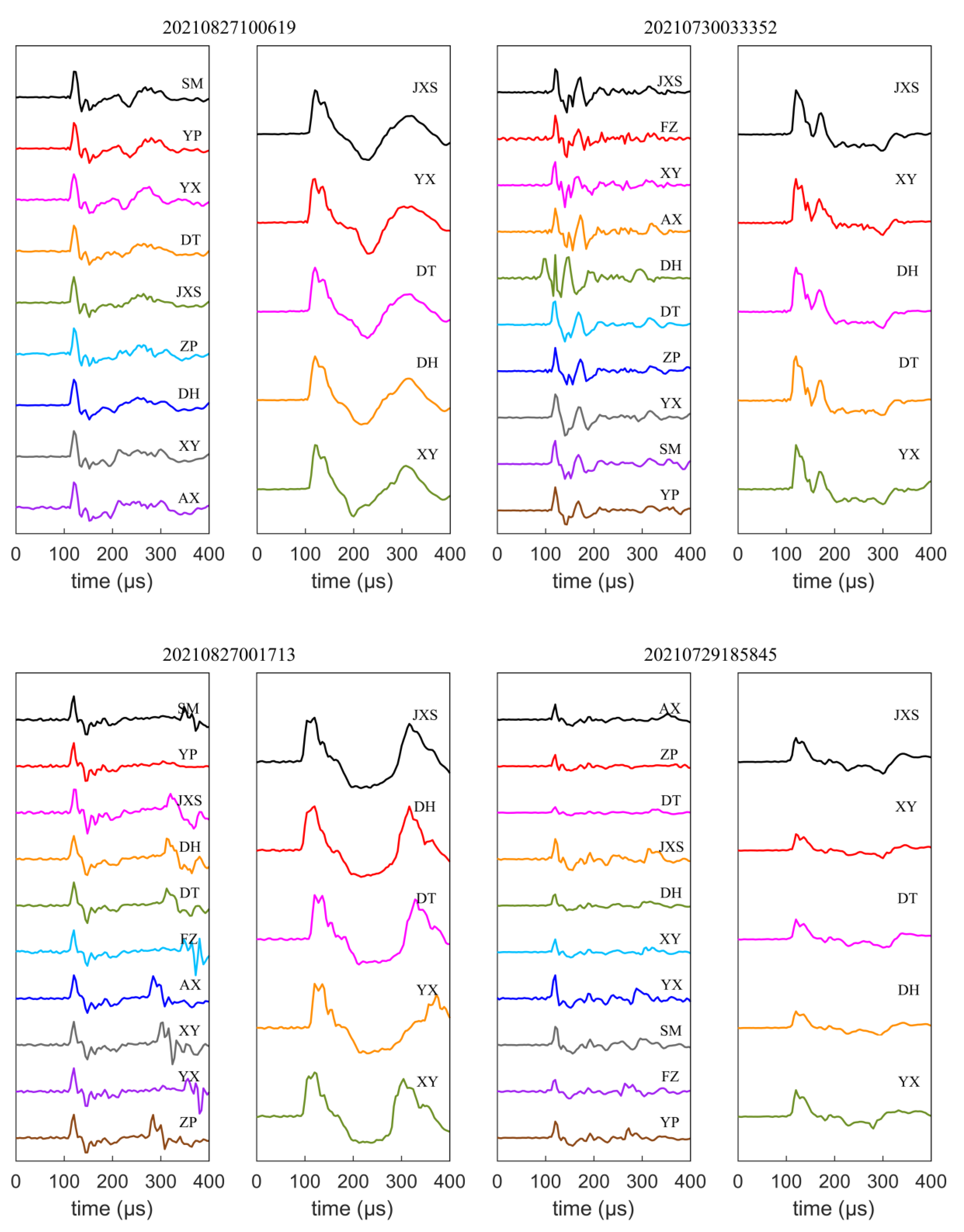
Figure 4 shows the reference location estimated by the ToA technique with arrival time differences using the time corresponding to the peak field (Tp). Due to limited space, reference location with the other two methods of arrival time differences is omitted. The hyperbolas of different colors are drawn corresponding to the arrival time differences between the center station (black triangle) and the station of same color as the hyperbola. It was found that the intersection region consisting of all hyperbolas was tight for all six cases, and the reference location (red cross) is located exactly in the tight intersection region. This can reflect the reliable synchronization of recorded data, the accurate method of arrival time differences and the validation of reference location.
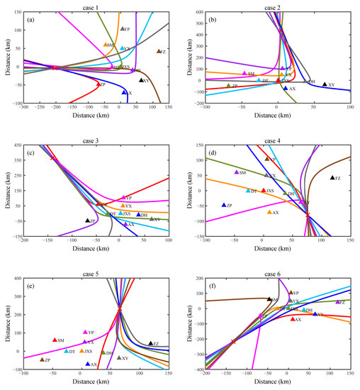
Figure 4.
The reference location of six cases estimated by the ToA technique with arrival time differences using the time corresponding to the peak field. (a–f) correspond to the results of case 1 to case 6. The hyperbolas of different colors correspond to the arrival time differences between the center station (black triangle) and the station of same color as the hyperbola. The red crosses mark the reference location.
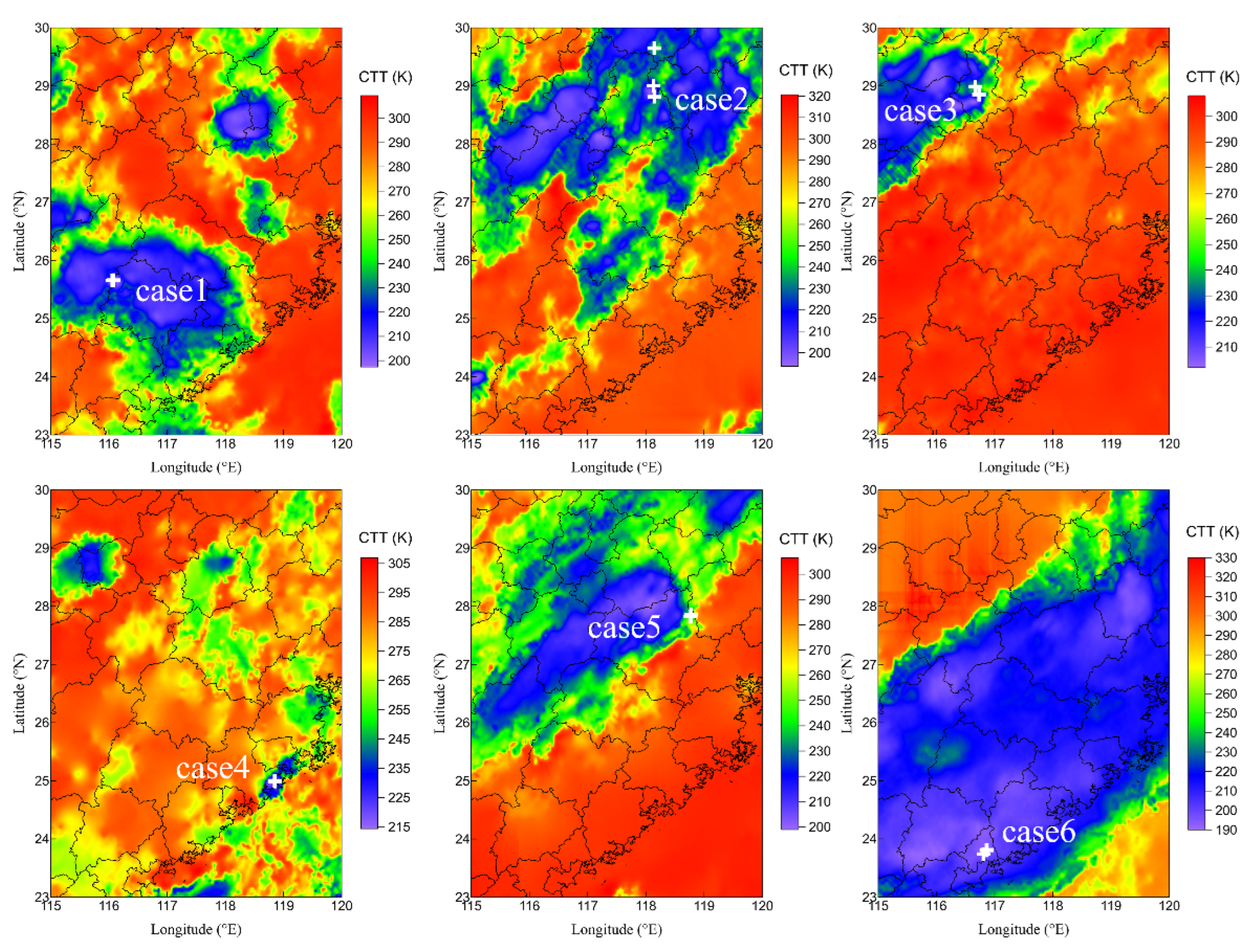
Figure 5 shows the reference locations of six cases estimated by the ToA technique with three methods of arrival time differences. The background is cloud top temperature (CTT) detected by the advanced geosynchronous radiation imager (AGRI) equipped by FY4A [45,46]. CTT was used in this study to investigate the development of convective clouds [47]. It can be seen that the reference locations are in the area of low CTT (i.e., strong convection), whatever the method of arrival time differences is. This strong dependence on the low CTT region provides convincing evidence that the reference locations are reasonable, although the exact lightning locations are unavailable. Due to the further propagation for case 2 and case 3, the arrival time determined by the two definitions (tp and t10) have certain differences. This difference was passed to the arrival time differences and finally affected the reference location result without affecting its validation.
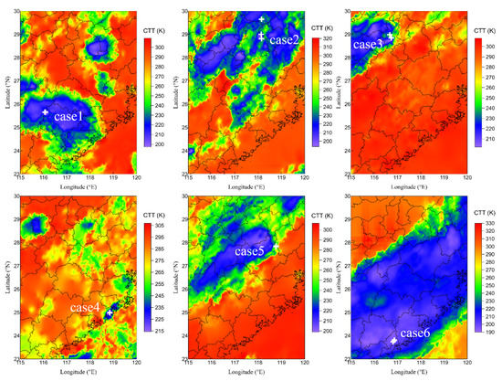
Figure 5.
The reference locations of six cases superimposed on the cloud top temperature map. The white crosses mark the reference locations estimated by the ToA technique with three methods of arrival time differences.
3.2. The Deviation Distance between the Reference Location and the Locations for Different Number and Configuration of Participating Stations
As mentioned in Section 2.2, three methods of arrival time differences were used to determine the lightning location, marked as Tp, T10 and Tcorr. The goodness-of-fit parameter χ2 is minimized when the lightning location is estimated, and the typical timing error σ2 in (2) was set to 1 μs [5,21]. As the number of synchronous magnetic field antennas was nine in case 2 and case 3, the maximum number of participating stations was eight, while the others were nine. The minimum number was five, because there are four unknowns in the non-linear equations. The locations are eliminated when its chi-square value was greater than 5 to avoid time gross error on the arrival time. Only the locations which pass the test could be compared with the reference location in the form of boxplots.
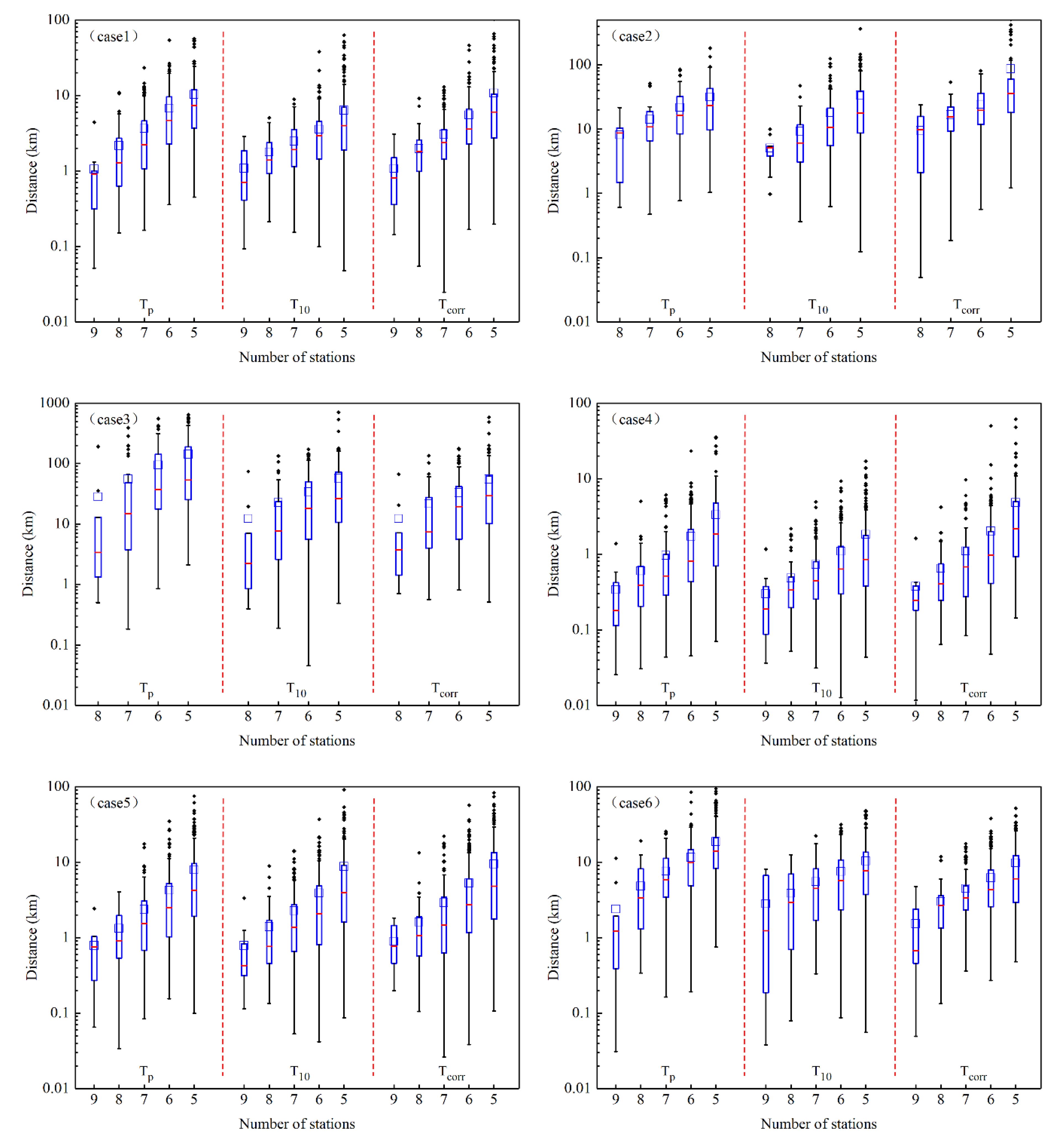
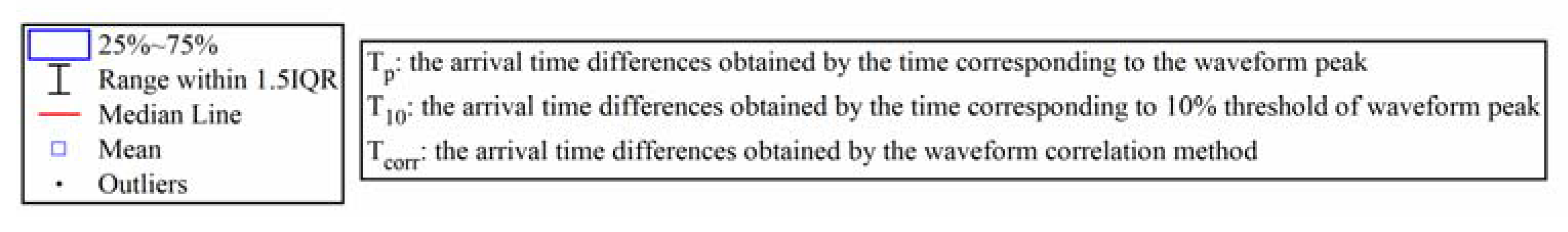
The results for the effect of number and configuration of participating stations on the quality of the lightning location outside the network are presented in Figure 6. The deviation distance between the reference location and the location under a different number and configuration of stations can be used to evaluate the impact of these two factors. It shows that the deviation distance decreases with the increase of number of participating stations and increases with the distance away from the network. It can be seen from the upper quartile (Q3), the lower quartile (Q1) and the median that the deviation distances obtained by the three definitions of arrival time difference (Tp, T10 and Tcorr) are not significantly different. Therefore, the deviation distance with the arrival time difference obtained by the time corresponding to the waveform peak was chosen to discuss two factors in the following text. When the number of stations was five, the deviation distance varies in between 0.07 and 424.7 km, with an average of 35 km while that for the number as eight is 0.03~21.6 km and 2.2 km, respectively. The next section will discuss the station configuration for the outliers in Figure 6 when the number of participating stations is five.
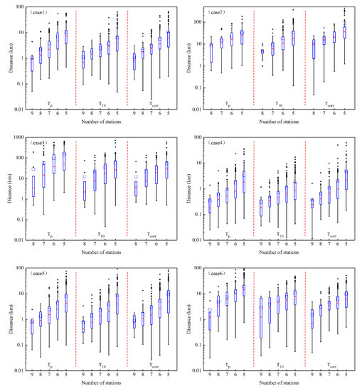
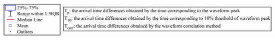
Figure 6.
The deviation distance of six cases between the reference location and the location under different number and configuration of stations using the ToA technique with three definitions of arrival time differences.
Figure 7 shows the spatial distribution of locations under different numbers and configurations of stations. It was found that the distribution of lightning locations become denser and closer to the reference location with the increase of number of participating stations for six cases outside the network. It is worth noting that the distribution of locations seems to be on a straight line. The direction of the distribution is consistent with the relative direction of the case to the network. For example, case 1 is located in the west of network, so its distribution is east–west. The reason for this distribution can be explained in the next section, taking the five participating stations as an example.
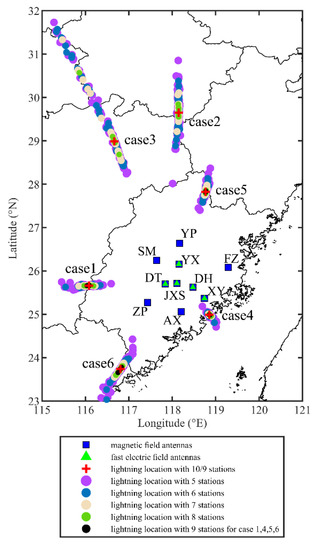
Figure 7.
The spatial distribution of locations under different numbers and configuration of participating stations. The red crosses represent the reference location, obtained by 10/9 stations. The purple, blue, misty rose, green, and black dots represent the locations obtained by 5, 6, 7, 8, 9 stations, respectively.
3.3. The Configuration of Five Stations under the Maximum and Minimum Deviation Distance
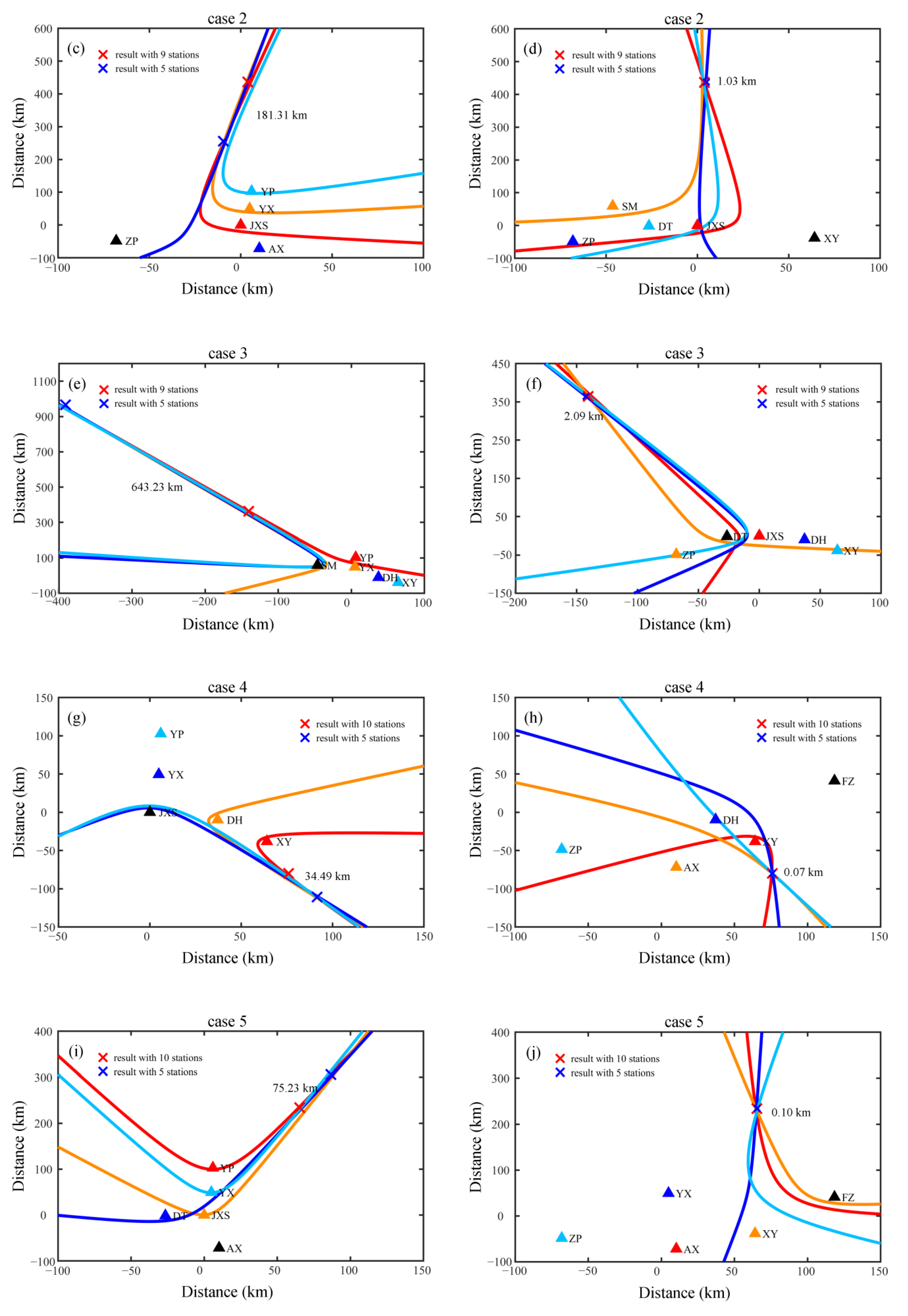
In this section, the configuration of five stations for six cases outside the network under the maximum and minimum deviation distance are shown in detail. There are four unknowns (x, y, z, t) in the non-linear equations and at least five stations are required to solve the equations using the least squares method. That’s the reason for choosing five stations to illustrate the effect of configuration.
Figure 8 shows the worst and best configurations corresponding to the maximum and minimum deviation distance. The value of these deviation distances for six cases is shown in Table 1. The left-side subplots describe the worst configurations for six cases. It was found that three participating stations approximately lied on a straight line, and the direction of the line is consistent with the direction of the case relative to the network. The linear configuration of three stations results in their hyperbolas being almost parallel to each other. The intersection region consisting of these almost parallel hyperbolas became narrow and long, not tight and focused on a point. In this situation, the fifth station was critical for finding the location where the minimum chi-square value was, using the least square method. The location was found at the intersection of the narrow long region and the hyperbola corresponding to the fifth station and significantly deviated from the reference location. For example, in Figure 8a of case 1, AX is the center station. DT, JXS and DH lay approximately on an east–west line, whose direction is the same as that of case 1 relative to the network. The red, yellow and blue hyperbolas corresponding to these three stations intersect and form a narrow long region. The cyan hyperbola corresponding to the fifth station XY intercepts this region, and their intersection (Figure 8a, blue cross) is the location under this configuration of five stations, being 63.49 km away from the reference location (Figure 8a, red cross).
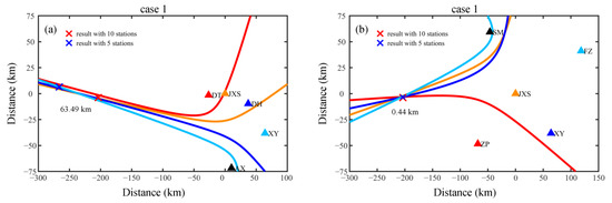
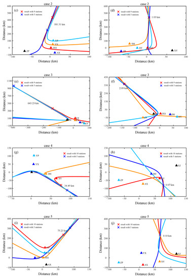
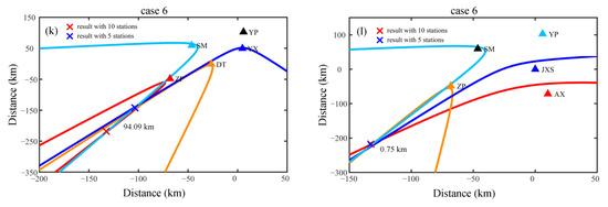
Figure 8.
The configuration of five stations under the maximum and minimum deviation distance for six cases. The left-side subplots describe the worst configurations while the right-side are the best configurations. (a,b) correspond to the results of case 1. (c,d) correspond to the results of case 2. (e,f) correspond to the results of case 3. (g,h) correspond to the results of case 4. (i,j) correspond to the results of case 5. (k,l) correspond to the results of case 6. The hyperbolas of different colors correspond to the arrival time differences between the center station (black triangle) and the station of same color as the hyperbola. The red crosses mark the reference location. The blue cross represents the location under the configuration of five stations.

Table 1.
The maximum and minimum deviation distances for six cases is with five stations.
The right-side subplots describe the best configurations for six cases. It is the more dispersed distribution of the participating stations that leads to the minimum deviation distance. The best configurations mean that no station lie on a straight line, at least on a line whose direction is the same as that of the case relative to the network. The narrow, long region mentioned in the last paragraph does not exist. The intersection region consisting of four hyperbolas is tight for all six cases. In Table 1, when the distance to each station is less than 270 km on average (i.e., case 1, 4, 5, 6), the minimum deviation distance is less than 1 km. When the distance to each station is about 430 km and 400 km on average (i.e., case 2, 3), the minimum deviation distance is 1 km and 2 km, respectively. It shows that under a specific configuration, the network consisting of five stations has the same performance as the network containing ten or nine stations, considering the deviation distance is less than 1 km.
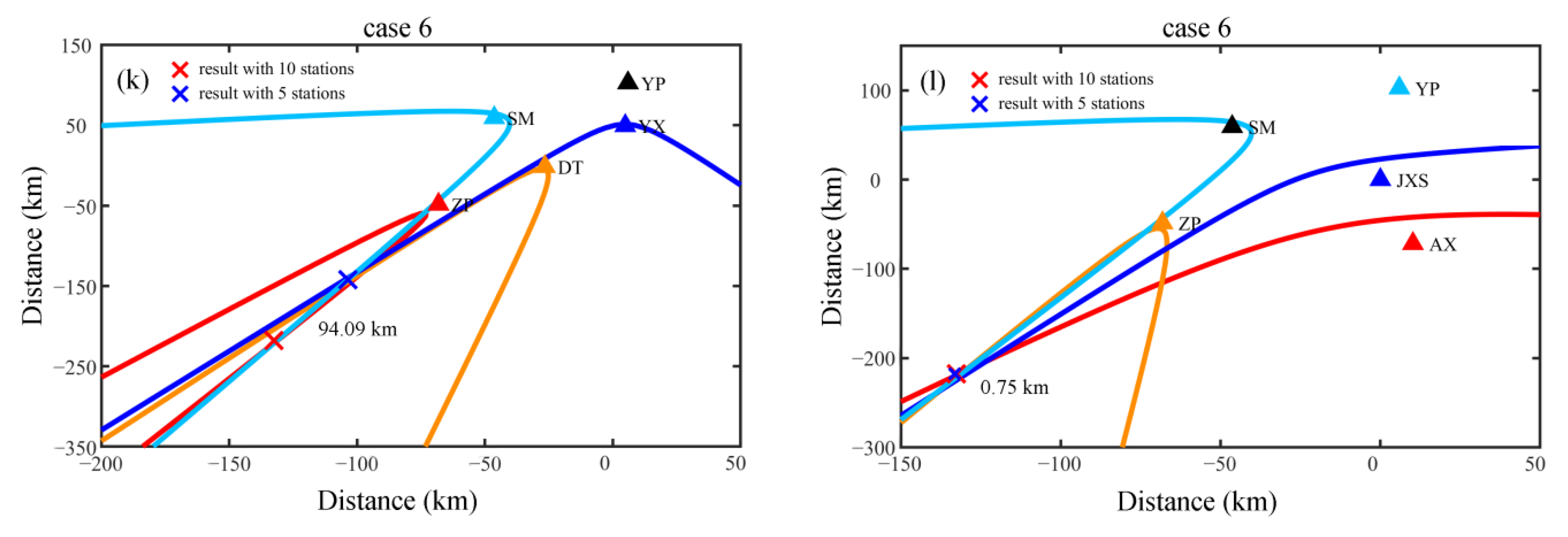
The station configurations for those outliers in Figure 6 are checked out, and the result is shown in Figure 9. The configuration with three or even four stations approximately lying on a straight line caused those outliers for six cases outside the network, especially when the direction of the line was nearly consistent with the direction of the case relative to the network. For case 1, the linear west–east distribution of the DT, JXS and DH station (Figure 9, red line) was the main reason for the outliers. For case 2 and case 5, the linear north–south distribution of YP, YX, JXS and AX station (Figure 9, blue line) is in existence. Arbitrarily, three of them or all of them participated in the location process, which explains the outliers. For case 3 and case 4, the linear distribution of YX, DH and XY stations (Figure 9, magenta line) is responsible for the appearance of outliers. The linear distribution of ZP, DT and YX stations (Figure 9, green line) and the linear north–south distribution (Figure 9, blue line) account for the outliers in case 6. Therefore, in order to avoid large deviation distance (outliers), the discrete configuration of stations rather than linear configuration, is selected for the increase of the number of stations.
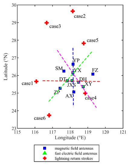
Figure 9.
The configuration with three or even four stations lying approximately on a straight line caused the outliers for six cases outside the network. The red line corresponds to the configuration for outliers of case 1. The blue line corresponds to the configuration for outliers of case 2 and case 5. The magenta line corresponds to the configuration for outliers of case 3 and case 4. The green line corresponds to the configuration for outliers of case 6.
This section will discuss the interpretation of the linear spatial distribution of locations under a different number and configuration of stations in Figure 7, taking the five participating stations as an example. No matter how large or small the deviation distance, the locations marked as purple dots seem to lie on a straight line, whose direction is consistent with the relative direction of the case to the network. The relative direction may account for the linear spatial distribution. Considering the distance between the case and the network is further than that between stations, the arrival direction of lightning discharge at each station is almost the same. Reversing the propagation direction (from the station to the lightning), it can be inferred that the lightning discharge must be along with this propagation direction and not in other directions. Note that linear distribution is a special phenomenon for lightning outside the network, but it does not exist for lightning inside the network.
4. Conclusions
According to the deviation distance boxplot and the spatial distribution map, the number and configuration of participating stations have an effect on lightning location outside the network. It is obvious that the more stations, the better lightning network performance. However, considering the establishment, maintenance and economic benefit of the lightning network, especially in mountainous areas, the appropriate number and reasonable position of stations are crucial in the early construction period.
The DE and LA are usually used to evaluate the performance of the lightning detection network. The DE is defined as the ratio between the number of lightning occurred and that located from the network. Due to the lack of large samples, DE is not discussed in this study. LA can be obtained by Monte Carlo simulation or objective evaluation based on artificially triggered lightning [31,34]. Several alternate methods have been used to show LA, such as relative performance with other LLS [35,36,48,49] and a comparison with radar reflectometry or cloud images observed from space [5,50,51]. Because the occurred lightning is unavailable and the location result from the other lightning networks is lacking in this study, the reference location using 10/9 stations waveforms data is regarded as the “occurred lightning” location and the deviation distance is regarded as “LA”. According to the six cases in different directions, the preliminary result for the LA outside the network can be obtained.
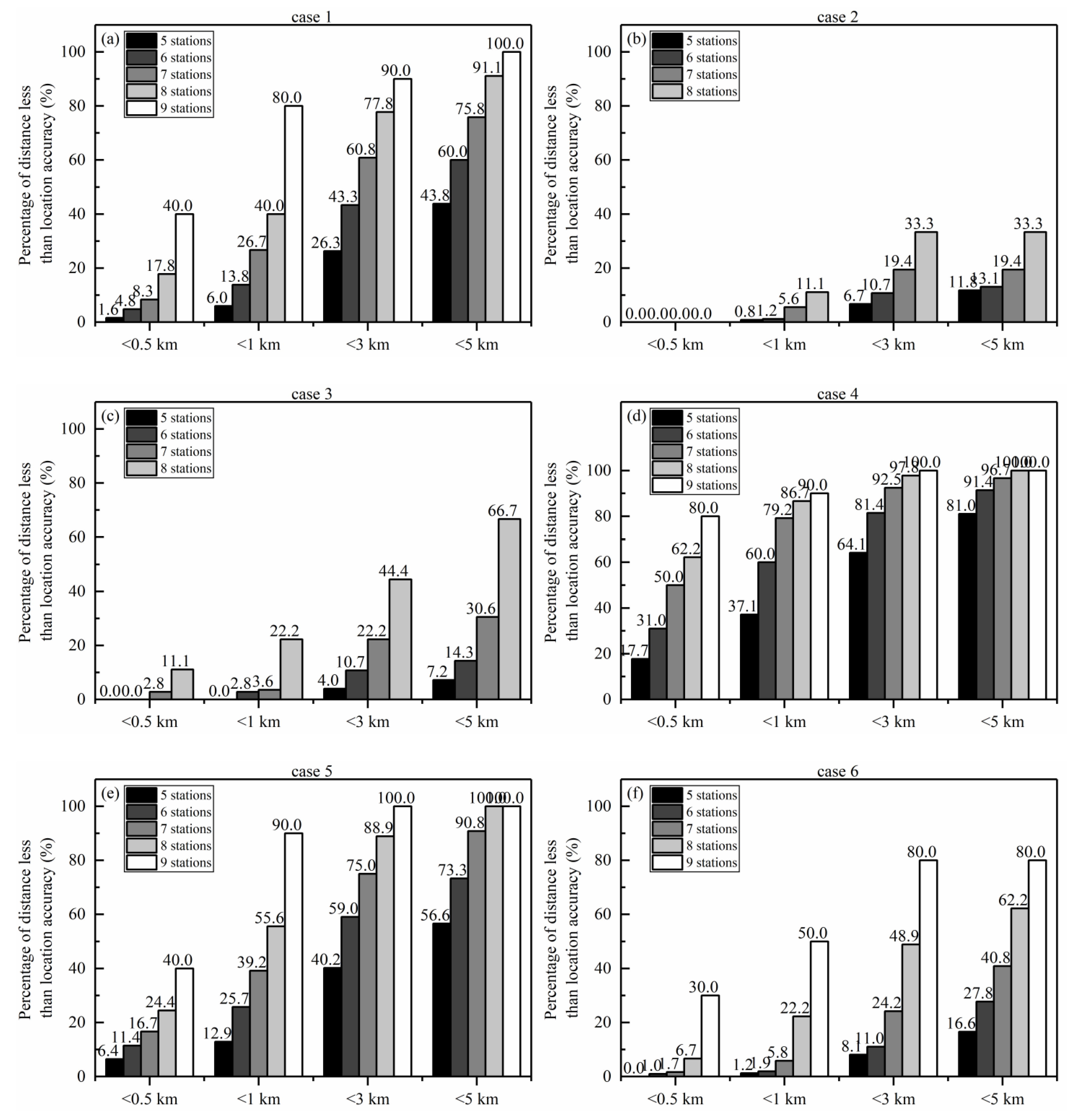
Figure 10 shows the percentage of deviation distance less than specific location accuracy for six cases with different numbers of participating stations. The percentage is the proportion of configurations with which the deviation distance satisfies the specific location accuracy to all configurations, which can provide references for the lightning network design. Case 4 occurred at the edge of the network, and the distance from each station is about 120 km on average. It can be seen in Figure 10d that when the number of stations is seven, the half of configurations can satisfy the location accuracy of 500 m. The percentage is about 80% when the deviation distance is less than 1 km with seven stations participating in location. It can be inferred that 7 stations are sufficient to accurately locate the lightning near and inside the network; more stations than are unnecessary. Case 1, 5 and 6 occurred at the outside of the network, and the distance from each station is about 220 km, 240 km, 270 km on average, respectively. It can be seen in Figure 10a,e,f that when the number of stations is nine, less than half of configurations can satisfy the location accuracy of 500 m, being 40%, 40% and 30%, respectively. With the location accuracy of 1 km, when the number of stations is nine, the percentage is about 80%, 90% and 50% for these three cases, respectively. For the location accuracy of 3 km, the percentage of case 1 is about 60% with seven stations and that of case 5 is also about 60% with six stations. However, the percentage of case 6 is less than 50% even with eight stations. For the location accuracy of 5 km, the percentage of case 1 is about 60% with six stations and that of case 5 is also about 73% with six stations. However, the percentage of case 6 is less than 50% even with seven stations. It can be inferred that 8–9 stations are necessary for LA of 1 km, 7–8 stations for LA of 3 km, 6–7 stations for LA of 5 km when the lightning occurred outside the network and was between 200–300 km away from the center of the network. Case 2 and 3 occurred at the outside network, and the distance to each station is about 430 km, 400 km on average, respectively. It can be seen from Figure 10b,c that when the number of stations is eight, less than half of configurations can satisfy the location accuracy of 500 m, 1 km or 3 km. For the location accuracy of 5 km, the percentage of case 3 is about 66% with eight stations and that of case 2 is about 33% with eight stations. It can be inferred that when the lightning occurred outside and at a distance of more than 400 km to the stations, the LA became very low, and the network is not suitable for locating such lightning. This paper only provides preliminary suggestions about the number and configuration of participating stations, according to the chosen six cases. In the future, more abundant detection data and location results from other LLSs can be used to improve the assessment of lightning network performance, including DE and LA.

Figure 10.
The percentage of deviation distance less than the specific location accuracy for six cases with different number of participating stations. (a–f) correspond to the results of case 1 to case 6.
In this paper, we established a regional lightning detection and location network in Fujian, China. Magnetic field antennas and fast electric field antennas working in VLF/LF band are equipped, and six cases detected by the network in 2021 summer from different directions are chosen to research the effect of number and configuration of participating stations on the quality of the lightning location outside the network. The ToA technique is used to determine the lightning location. The reference location is validated by the tight intersection region consisting of all hyperbolas and by the close correlation with the low cloud top temperature region. The deviation distance between the reference location and the locations for different number and configuration of stations decrease with the increase of number of participating stations and increase with the distance away from the network. The main conclusions are summarized as follows.
When the number of stations was five, the deviation distance varied from 0.07 to 424.7 km, with an average of 35 km while that for the number being eight is 0.03~21.6 km and 2.2 km, respectively. The spatial distribution of those locations outside the network seemed to be on a straight line and become denser and closer to the reference location with the increase of number of stations. When the number of participating stations was five, the station linear configuration led to a narrow and long intersection region, where the final location is determined by finding the minimum chi-square value using the least square method, resulting in the large deviation distance. This is the explanation for the outliers of six cases. The more dispersed distribution of the participating stations leads to the minimum deviation distance for six cases. The percentage of deviation distance less than specific location accuracy can provide references for the lightning network design. Seven stations were sufficient to accurately locate the lightning near and inside the network. When lightning occurred outside the network and the distance was between 200 to 300 km with respect to the center of the network, 8–9 stations were necessary for LA of 1 km, 7–8 stations for LA of 3 km and 6–7 stations for LA of 5 km. When the distance of lightning to the stations was more than 400 km on average, the LA became very low, and the network was not suitable for locating the lightning.
Author Contributions
Conceptualization, J.G. and Q.Z.; Methodology, J.G. and Q.Z.; Software, J.G., J.L. and J.Z. (Junchao Zhang); Validation, J.G.; Formal analysis, J.G., J.L. and J.Y.; Investigation, J.G., Q.Z.; Resources, Q.Z.; Data curation, J.Z. (Jiahao Zhou), B.D., H.S., Y.W., J.W., Y.Z. and Q.L.; Writing—original draft preparation, J.G.; Writing—review and editing, Q.Z.; Visualization, J.G.; Supervision, Q.Z.; Project administration, Q.Z. Funding acquisition, Q.Z. All authors have read and agreed to the published version of the manuscript.
Funding
This research was funded by the National Key R&D Program of China under Grant 2017YFC1501505, in part by the National Natural Science Foundation of China under Grant 41775006.
Data Availability Statement
Not applicable.
Conflicts of Interest
The authors declare no conflict of interest.
Abbreviations
| AGRI | advanced geosynchronous radiation imager |
| AX | Anxi station |
| BLNET | Beijing Lightning Network |
| BOLT | Broadband Observation Network for Lightning and Thunderstorm positioning system |
| CTT | Cloud-Top Temperature |
| DE | detection efficiency |
| DH | Dehua station |
| DT | Datian station |
| EUCLID | European Cooperation for Lightning Detection |
| FALMA | Fast Antenna Lightning Mapping Array |
| FY4A | FengYun 4A meteorological satellite |
| FZ | Fuzhou station |
| GPS | Global Positioning System |
| IBP | initial breakdown processes |
| IC | intracloud lightning |
| JASA | Jianghuai Area Sferic Array |
| JXS | Jiuxianshan station |
| LA | location accuracy |
| LASA | Los Alamos Sferic Array |
| LDAR | Lightning Detection and Ranging |
| LF | low frequency |
| LFEDA | Low-frequency E-field Detection Array |
| LINET | Lightning detection network |
| LLSs | lightning location systems |
| LMA | Lightning Mapping Array |
| NBE | narrow bipolar event |
| NLDN | National Lightning Detection Network |
| SM | Sanming station |
| ToA | time of arrival |
| VHF | very high frequency |
| VLF | very low frequency |
| XY | Xianyou station |
| YP | Yanping station |
| YX | Youxi station |
| ZP | Zhangping station |
References
- Rakov, V.A.; Uman, M.A. Lightning: Physics and Effects; Cambridge University Press: Cambidge, UK, 2003. [Google Scholar]
- Cummins, K.L.; Murphy, M.J.; Bardo, E.A.; Hiscox, W.L.; Pyle, R.B.; Pifer, A.E. A combined TOA/MDF technology upgrade of the US National Lightning Detection Network. J. Geophys. Res. Atmos. 1998, 103, 9035–9044. [Google Scholar] [CrossRef]
- Cummins, K.L.; Murphy, M.J. An Overview of Lightning Locating Systems: History, Techniques, and Data Uses, With an In-Depth Look at the U.S. NLDN. IEEE Trans. Electromagn. Compat. 2009, 51, 499–518. [Google Scholar] [CrossRef]
- Smith, D.A.; Eack, K.B.; Harlin, J.; Heavner, M.J.; Jacobson, A.R.; Massey, R.S.; Shao, X.M.; Wiens, K.C. The Los Alamos Sferic Array: A research tool for lightning investigations. J. Geophys. Res. Atmos. 2002, 107, ACL-5. [Google Scholar] [CrossRef]
- Shao, X.M.; Stanley, M.; Regan, A.; Harlin, J.; Pongratz, M.; Stock, M. Total lightning observations with the new and improved Los Alamos Sferic Array (LASA). J. Atmos. Oceanic Technol. 2006, 23, 1273–1288. [Google Scholar] [CrossRef]
- Betz, H.D.; Schmidt, K.; Laroche, P.; Blanchet, P.; Oettinger, W.P.; Defer, E.; Dziewit, Z.; Konarski, J. LINET—An international lightning detection network in Europe. Atmos. Res. 2009, 91, 564–573. [Google Scholar] [CrossRef]
- Betz, H.D.; Meneux, B. LINET systems—10 years experience. In Proceedings of the IEEE 2014 International Conference on Lightning Protection (ICLP), Shanghai, China, 11–18 October 2014. [Google Scholar] [CrossRef]
- Liu, C.; Heckman, S. Using total lightning data in severe storm prediction: Global case study analysis from North America, Brazil and Australia. In Proceedings of the 2011 International Symposium on Lightning Protection (XI SIPDA), Fortaleza, Brazil, 3–7 October 2011. [Google Scholar] [CrossRef]
- Schulz, W.; Diendorfer, G.; Pedeboy, S.; Poelman, D.R. The European lightning location system EUCLID—Part 1: Performance analysis and validation. Nat. Hazards Earth Syst. Sci. 2016, 16, 595–605. [Google Scholar] [CrossRef]
- Dowden, R.L.; Holzworth, R.H.; Rodger, C.J.; Lichtenberger, J.; Thomson, N.R.; Jacobson, A.R.; Lay, E.; Brundell, J.B.; Lyons, T.J.; O’keefe, S. World-Wide Lightning Location Using VLF Propagation in the Earth-Ionosphere Waveguide. IEEE Antennnas Propag. Mag. 2008, 50, 40–60. [Google Scholar] [CrossRef]
- Rodger, C.J.; Werner, S.W.; Brundell, J.B.; Thomas, N.R.; Lay, E.H.; Holzworth, R.H.; Dowden, R.L. Detection efficiency of the VLF World-Wide Lightning Location Network (WWLLN): Initial case study. Ann. Geophys. 2004, 24, 3197–3214. [Google Scholar] [CrossRef] [Green Version]
- Said, R.K.; Inan, U.S.; Cummins, K.L. Long-Range Lightning Geolocation Using a VLF Radio Atmospheric Waveform Bank. J. Geophys. Res. 2010, 115, D23108. [Google Scholar] [CrossRef]
- Pessi, A.T.; Businger, S.; Cummins, K.L.; Demetriades, N.W.S.; Murphy, M.; Pifer, B. Development of a Long-Range Lightning Detection Network for the Pacific: Construction, Calibration, and Performance. J. Atmos. Ocean. Tech. 2009, 26, 145–166. [Google Scholar] [CrossRef]
- Chronis, T.G.; Anagnostou, E.N. Error Analysis for a Long-Range Lightning Monitoring Network of Ground-Based Receivers in Europe. J. Geophys. Res. 2003, 108, 1–10. [Google Scholar] [CrossRef]
- Rustan, P.L.; Uman, M.A.; Childers, D.G.; Beasley, W.H.; Lennon, C.L. Lightning source locations from VHF radiation data for a flash at Kennedy Space Center. J. Geophys. Res. Oceans 1980, 85, 4893–4903. [Google Scholar] [CrossRef]
- Thomas, R.J.; Krehbiel, P.R.; Rison, W.; Hunyady, S.J.; Winn, W.P.; Hamlin, T.; Harlin, J. Accuracy of the Lightning Mapping Array. J. Geophys. Res. 2004, 109, D14207. [Google Scholar] [CrossRef]
- Shao, X.M.; Holden, D.N.; Rhodes, C.T. Broad band radio interferometry for lightning observations. Geophys. Res. Lett. 1996, 23, 1917–1920. [Google Scholar] [CrossRef]
- Yoshida, S.; Biagi, C.J.; Rakov, V.A.; Hill, J.D.; Stapleton, M.V.; Jordan, D.M.; Uman, M.A.; Morimoto, T.; Ushio, T.; Kawasaki, Z.I. Three-dimensional imaging of upward positive leaders in triggered lightning using VHF broadband digital interferometers. Geophys. Res. Lett. 2010, 37, L05805. [Google Scholar] [CrossRef]
- Stock, M.G.; Akita, M.; Krehbiel, P.R.; Rison, W.; Edens, H.E.; Kawasaki, Z.; Stanley, M.A. Continuous broadband digital interferometry of lightning using a generalized cross—Correlation algorithm. J. Geophys. Res. Atmos. 2014, 119, 3134–3165. [Google Scholar] [CrossRef]
- Karunarathne, S.; Marshall, T.C.; Stolzenburg, M.; Karunarathna, N.; Vickers, L.E.; Warner, T.A.; Orville, R.E. Locating initial breakdown pulses using electric field change network. J. Geophys. Res. Atmos. 2013, 118, 7129–7141. [Google Scholar] [CrossRef]
- Bitzer, P.M.; Christian, H.J.; Stewart, M.; Burchfield, J.; Podgorny, S.; Corredor, D.; Hall, J.; Kuznetsov, E.; Franklin, V. Characterization and applications of VLF/LF source locations from lightning using the Huntsville Alabama Marx Meter Array. J. Geophys. Res. Atmos. 2013, 118, 3120–3138. [Google Scholar] [CrossRef]
- Zhu, Y.; Bitzer, P.M.; Stewart, M.; Podgorny, S.; Corredor, D.; Burchfeld, J.; Carey, L.; Medina, B.; Stock, M. Huntsville Alabama Marx meter array 2: Upgrade and capability. Earth Space Sci. 2020, 7, e2020EA001111. [Google Scholar] [CrossRef]
- Lyu, F.C.; Cummer, S.A.; Solanki, R.; Weinert, J.; McTague, L.; Katko, A.; Barrett, J.; Zigoneanu, L.; Xie, Y.; Wang, W. A low-frequency near-field interferometric-TOA 3-D Lightning Mapping Array. Geophys. Res. Lett. 2014, 41, 7777–7784. [Google Scholar] [CrossRef]
- Yoshida, S.; Wu, T.; Ushio, T.; Kusunoki, K.; Nakamura, Y. Initial results of LF sensor network for lightning observation and characteristics of lightning emission in LF band. J. Geophys. Res. Atmos. 2014, 119, 12034–12051. [Google Scholar] [CrossRef]
- Ushio, T.; Wu, T.; Yoshida, S. Review of recent progress in lightning and thunderstorm detection techniques in Asia. Atmos. Res. 2015, 154, 89–102. [Google Scholar] [CrossRef]
- Wu, T.; Wang, D.H.; Takagi, N. Lightning mapping with an array of fast antennas. Geophys. Res. Lett. 2018, 45, 3698–3705. [Google Scholar] [CrossRef]
- Wang, J.; Huang, Q.; Ma, Q.; Chang, S.; He, J.; Wang, H.; Zhou, X.; Xiao, F.; Gao, C. Classification of VLF/LF Lightning Signals Using Sensors and Deep Learning Methods. Sensors 2020, 20, 1030. [Google Scholar] [CrossRef]
- Chen, S.; Du, Y.; Fan, L.; He, H.; Zhong, D. A lightning location system in China: Its performances and applications. IEEE Trans. Electromagn. Compat. 2002, 44, 555–560. [Google Scholar] [CrossRef]
- Wang, Y.; Qie, X.; Wang, D.; Liu, M.; Su, D.; Wang, Z.; Liu, D.; Wu, Z.; Sun, Z.; Tian, Y. Beijing Lightning Network (BLNET) and the observation on preliminary breakdown processes. Atmos. Res. 2016, 171, 121–132. [Google Scholar] [CrossRef]
- Yuan, S.; Qie, X.; Jiang, R.; Wang, D.; Sun, Z.; Srivastava, A.; Williams, E. Origin of an uncommon multiple-stroke positive cloud-to-ground lightning flash with different terminations. J. Geophys. Res. Atmos. 2020, 125, e2019JD032098. [Google Scholar] [CrossRef]
- Shi, D.; Zheng, D.; Zhang, Y.; Zhang, Y.; Huang, Z.; Lyu, W.; Chen, S.; Yan, X. Low-frequency E-field Detection Array (LFEDA)—Construction and preliminary results. Sci. China Earth Sci. 2017, 60, 1896–1908. [Google Scholar] [CrossRef]
- Qin, Z.; Zhu, B.; Lyu, F.; Ma, M.; Ma, D. Using time domain waveforms of return strokes to retrieve the daytime fluctuation of ionospheric D layer. Chin. Sci. Bull. 2015, 60, 654–663. [Google Scholar] [CrossRef]
- Liu, F.; Qin, Z.; Zhu, B.; Ma, M.; Chen, M.; Shen, P. Observations of ionospheric D layer fluctuations during sunrise and sunset by using time domain waveforms of lightning narrow bipolar events. Chin. J. Geophys. 2018, 61, 484–493. [Google Scholar] [CrossRef]
- Ma, Z.; Jiang, R.; Qie, X.; Xing, H.; Liu, M.; Sun, Z.; Qin, Z.; Zhang, H.; Li, X. A low frequency 3D lightning mapping network in north China. Atmos. Res. 2020, 249, 105314. [Google Scholar] [CrossRef]
- Pohjola, H.; Mäkelä, A. The comparison of GLD360 and EUCLID lightning location systems in Europe. Atmos. Res. 2013, 123, 117–128. [Google Scholar] [CrossRef]
- Kuk, B.J.; Kim, H.I.; Ha, J.S.; Lee, H.K. Intercomparison study of cloud-to-ground lightning flashes observed by KARITLDS and KLDN at South Korea. J. Appl. Meteorol. Climatol. 2010, 50, 224–232. [Google Scholar] [CrossRef]
- Srivastava, A.; Tian, Y.; Qie, X.; Wang, D.; Sun, Z.; Yuan, S.; Wang, Y.; Chen, Z.; Xu, W.; Zhang, H.; et al. Performance Assessment of Beijing Lightning Network (BLNET) and Comparison with Other Lightning Location Networks across Beijing. Atmos. Res. 2017, 197, 76–83. [Google Scholar] [CrossRef]
- Cooray, V. Propagation effects due to finitely conducting ground on lightning-generated magnetic fields evaluated using Sommerfeld’s integrals. IEEE Trans. Electromagn. Compat. 2009, 51, 526–531. [Google Scholar] [CrossRef]
- Zhang, Q.; Ji, T.; Hou, W. Effect of frequency-dependent soil on the propagation of electromagnetic fields radiated by subsequent lightning strike to tall objects. IEEE Trans. Electromagn. Compat. 2015, 57, 112–120. [Google Scholar] [CrossRef]
- Zhang, Q.; Yang, J.; Jing, X.; Li, D.; Wang, Z. Propagation effect of a fractal rough ground boundary on the lightning-radiated vertical electric field. Atmos. Res. 2012, 104, 202–208. [Google Scholar] [CrossRef]
- Li, D.; Rubinstein, M.; Rachidi, F.; Diendorfer, G.; Schulz, W.; Lu, G. Location Accuracy Evaluation of ToA-Based Lightning Location Systems Over Mountainous Terrain. J. Geophys. Res. Atmos. 2017, 122, 11760–11775. [Google Scholar] [CrossRef]
- Koshak, W.J.; Solakiewicz, R.J.; Blakeslee, R.J.; Goodman, S.J.; Christian, H.J.; Hall, J.M.; Bailey, J.C.; Krider, E.P.; Bateman, M.G.; Boccippio, D.J.; et al. North Alabama lightning mapping array (LMA): VHF source retrieval algorithm and error analyses. J. Atmos. Ocean Technol. 2004, 21, 543–558. [Google Scholar] [CrossRef]
- Chan, Y.T.; Ho, K.C. A simple and efficient estimator for hyperbolic location. IEEE Trans. Signal Process. 1994, 42, 1905–1915. [Google Scholar] [CrossRef]
- Schulz, W. Performance Evaluation of Lightning Location Systems. Ph.D. Thesis, Department of Electrical Engineering at the Technical University of Vienna, Vienna, Austria, 1997. [Google Scholar]
- Min, M.; Wu, C.; Li, C.; Liu, H.; Xu, N.; Wu, X.; Chen, L.; Wang, F.; Sun, F.; Qin, D.; et al. Developing the science product algorithm testbed for Chinese next-generation geostationary meteorological satellites: Fengyun-4 series. J. Meteorol. Res. 2017, 31, 708–719. [Google Scholar] [CrossRef]
- Zhang, P.; Zhu, L.; Tang, S.; Gao, L.; Chen, L.; Zheng, W.; Han, X.; Chen, J.; Shao, J. General Comparison of FY-4A/AGRI with Other GEO/LEO Instruments and Its Potential and Challenges in Non-meteorological Applications. Front. Earth Sci. 2019, 6, 224. [Google Scholar] [CrossRef]
- Yang, J.; Wang, Z.; Heymsfield, A.J.; DeMott, P.J.; Twohy, C.H.; Suski, K.J.; Toohey, D.W. High Ice Concentration Observed in Tropical Maritime Stratiform Mixed-Phase Clouds with Top Temperatures Warmer than −8 °C. Atmos. Res. 2020, 233, 104719. [Google Scholar] [CrossRef]
- Jacobson, A.R.; Holzworth, R.; Harlin, J.; Dowden, R.; Lay, E. Performance assessment of the World Wide Lightning Location Network (WWLLN), using the Los Alamos Sferic Array (LASA) as ground truth. J. Atmos. Ocean. Technol. 2006, 23, 1082–1092. [Google Scholar] [CrossRef]
- Abreu, D.; Chandan, D.; Holzworth, R.H.; Strong, K.A. performance assessment of the World Wide Lightning Location Network (WWLLN) via comparison with the Canadian Lightning Detection Network (CLDN). Atmos. Meas. Tech. 2010, 3, 1143–1153. [Google Scholar] [CrossRef]
- Liu, D.; Qie, X.; Xiong, Y.; Feng, G. Evolution of the total lightning activity in a leading line and trailing stratiform mesoscale convective system over Beijing. Adv. Atmos. Sci. 2011, 28, 866–878. [Google Scholar] [CrossRef]
- Wang, F.; Qie, X.; Liu, D.; Shi, H.; Srivastava, A. Lightning activity and its relationship with typhoon intensity and vertical wind shear for super typhoon Haiyan (1330). J. Meteorol. Res. 2016, 30, 117–127. [Google Scholar] [CrossRef]

Publisher’s Note: MDPI stays neutral with regard to jurisdictional claims in published maps and institutional affiliations. |
© 2022 by the authors. Licensee MDPI, Basel, Switzerland. This article is an open access article distributed under the terms and conditions of the Creative Commons Attribution (CC BY) license (https://creativecommons.org/licenses/by/4.0/).