Article

Measuring Land Surface Deformation over Soft Clay Area Based on an FIPR SAR Interferometry Algorithm—A Case Study of Beijing Capital International Airport (China)

1
School of Traffic and Transportation Engineering, Changsha University of Science and Technology, Changsha 410114, China
2
Hunan Key Laboratory of Remote Sensing of Ecological Environment in Dongting Lake Area, Changsha 410114, China
3
Laboratory of Radar Remote Sensing Applications, Changsha University of Science and Technology, Changsha 410014, China
4
Hunan International Scientific and Technological Innovation Cooperation Base of Advanced Construction and Maintenance Technology of Highway, Changsha University of Science & Technology, Changsha 410114, China
5
School of Geosciences and Info-physics, Central South University, Changsha 410083, China
6
Engineering Laboratory of Spatial Information Technology of Highway Geological Disaster Early Warning in Hunan Province, Changsha University of Science & Technology, Changsha 410114, China
*
Author to whom correspondence should be addressed.
Remote Sens. 2022, 14(17), 4253; https://doi.org/10.3390/rs14174253
Submission received: 13 July 2022 / Revised: 19 August 2022 / Accepted: 24 August 2022 / Published: 29 August 2022
(This article belongs to the Special Issue Geodetic Monitoring for Land Deformation)

Abstract

:
Long-term settlement monitoring of infrastructure built in soft clay areas is of great importance. When using InSAR technology for soft clay settlement monitoring, deformation modeling is a key process. In most InSAR deformation modeling, each component of the total deformation is expressed directly with a fixed functional model in phase functions and assumed to occupy an equal weight. This causes equal weight assumption uncertainty and ignores the actual certain contribution of each phase component related to certain deformational factors. Moreover, the commonly used mathematical empirical models in traditional InSAR are not suitable for describing the nonlinear characteristics of the temporal settlement evolution for soft clay. To address these limitations, we propose an SAR interferometry algorithm, namely, FIPR (FastICA Poisson-curve reciprocal accumulation method), which separates the original InSAR signal based on FastICA to extract each deformation component, and then the models can each extract deformation components and estimate the unknown parameters based on a reciprocal accumulation method. Each independent component and the obtained deformation parameters are used to generate the final deformation time series. Both simulated and real data experiments were designed. The simulated experimental results indicated that the sICA (spatial independent component analysis) separated results were much closer to the original signals than those of the tICA (temporal independent component analysis), with their RMSE lower than 2 mm, and the sICA is thus more highly recommended. Beijing Capital International Airport in China was selected as the study area in the real data experiment. Using 24 high-resolution TerraSAR-X radar satellite images from January 2012 to February 2015, the time-series deformation was obtained, with the maximum cumulative subsidence of 126 mm. The modeling accuracy for the proposed model was estimated as ±2.6 mm, with an improvement of 36.6% compared to the EWA-LM (linear model with equal weight accumulation) algorithm and 16.1% compared to the EWA-PC (Poisson curve with equal weight accumulation) algorithm. The RMSE with external leveling measurements was estimated as ±1.0 mm, with 69.7% improvement compared to EWA-LM and 50% to EWA-PC. This indicated that FIPR can reduce the uncertainty of artificial assumptions in deformation modeling and improve the accuracy of deformation analysis for highways in soft clay areas, providing a reference for road maintenance and management.

Graphical Abstract

1. Introduction

Long-term settlement monitoring of soft clay in urban areas is of great significance in preventing urban safety accidents and ensuring the quality of urban engineering construction [1,2,3,4]. Interferometric Synthetic Aperture Radar (InSAR) has been widely applied to ground surface movement monitoring with its advantages of large spatial coverage, high imaging resolution, and non-intrusive surveying. MT-InSAR (Multi-temporal Interferometric Synthetic Aperture Radar) technology, represented by persistent scatterer InSAR (PSI) [5], small baseline subsets InSAR (SBAS-InSAR) [6], and other advanced InSAR techniques, with its advantages of large spatial coverage, non-contact observation, and high accuracy for earth observation, has been proven to possess high capability in large urban infrastructure monitoring [7,8,9,10,11,12,13].
In InSAR data processing, deformation modeling is a crucial step. Most InSAR deformation models used for highway deformation monitoring are single mathematical empirical models (such as linear models [6], seasonal models [14], polynomial models [15], etc.) or their combinations, which ignore the specific deformation mechanisms of soft clays and are not able to describe the real temporal displacement law of the soft soil. This may affect the accuracy of the final derived deformation time series and counteract the subsequent highway deformation prediction and interpretation during the post-construction period. To correct these deficiencies, Zhu et al. proposed a temporal InSAR deformation model based on Poisson’s curve and successfully implemented it in the soft clay highway deformation estimation, which showed an accuracy improvement of 67% compared to the traditional InSAR model [16]. However, in the study, each deformation component, such as the Poisson model-related component and the linear component, was directly superimposed on the established InSAR phase functions under the assumption of equal weights. Actually, the information of the differential interference phase was considerably complex, so the simple equal weight composition for all the deformation components under the equal weight assumption could not reflect the actual characteristics of deformation composition and introduced uncertainties and errors. If each signal in the InSAR phase can be accurately separated, accurate deformation-related components can be extracted and then modeled according to the displacement characteristics, the significance of the model will be enhanced, and the accuracy of the final acquired deformation will be greatly improved.
Independent component analysis (ICA) is a commonly used blind signal separation (BSS) technique employed to decompose mixed random signals into linear combinations of independent components. It has been widely used in image extraction [17], seismic wave decomposition [18], and measurement data processing [19,20,21,22,23,24]. Scholars have applied ICA to the separation of the InSAR phase and deformation signals to assist in the analysis of geophysical phenomena. Bellator successfully used ICA to extract the digital elevation models from SAR data [25]; Ebmeier et al. applied ICA in InSAR volcano monitoring [26] and proved that ICA was capable of analyzing and separating volcanic signals accurately, even under atmospheric noise interference situations; Gaddes et al. applied ICA to the 2015 Wolf volcanic eruption and developed an algorithm based on ICA technique to identify the volcanic eruptions [27]; Peng et al. utilized ICA in the separation of the mixed InSAR time-series signals and proved that ICA could not only reveal the existence of two different spatio-temporal deformation characteristics in the Willcox Basin but also filter the residuals in InSAR observations [28]. The above studies fully validated the feasibility and reliability of the idea that introducing ICA for InSAR phase separation can assist the subsequent deformation extraction and analysis.
To compensate for the uncertainty of artificial assumptions with equal weight modeling in traditional InSAR data processing and to improve the accuracy of deformation estimation, we propose an ICA-based deformation estimation method for soft clay regions—FIPR (FastICA Poisson-curve reciprocal accumulation method). First, we use the FastICA algorithm to separate the original InSAR signals to extract and analyze the deformation signals in InSAR data. Then, we use the Poisson curve to model the extracted deformation components and the periodic function to model the environment-related components, and, we then introduce the reciprocal accumulation algorithm to estimate the model parameters. Finally, we obtain the total time-series deformation results. The FIPR SAR Interferometry Algorithm proposed here can achieve high-accuracy in deformation monitoring and future deformation prediction. The proposed method can assist in revealing the information of deformational magnitude, boundary of occurred scope and area, suggesting potential risk areas and suspected hidden danger points, identifying the occurred and potential geological disaster areas to a certain extent, and providing guidance for the related government and constructions to carry out in-situ emphasis of monitoring areas.

2. Methodology

2.1. InSAR Signal Separation Based on FastICA

ICA is a data-driven method based on blind source separation. Its basic principle is to separate the multi-channel observation signals into statistically independent components according to a certain optimization criterion method [29,30]. Compared with the model-driven method, it can effectively detect signal features without any prior conditions, such as a functional model and the weight of each independent variable [31]. Ebmeier et al. proved that in the interferogram formed by the complex conjugation of two SAR radar images, each pixel can be regarded as a linear combination of specific points and noise signals in the time series of multiple potential deformation sources [26]. If these noise signals and deformation sources are statistically independent, spatially and temporally, the restoration of the original signal can be regarded as the problem of blind source separation. The relationship between the InSAR time-series phase signals and the independent components can be expressed as:
X = A   ·   S
where X is the obtained unwrapped temporal InSAR phase signals; A is the mixing matrix, where the rows represent the spatial responses of the independent components; S is the independent component matrix, where each row represents an independent component.
The original InSAR data are a set of image sequences that should be squeezed into a two-dimensional matrix X ·( M × N p i x e l ) in spatial ICA (sICA) or X ·( N p i x e l × M ) in temporal ICA (tICA) processing. The different arrangement of X determines that ICA has different detection methods in the response domain of InSAR data. sICA considers that multiple regions related to deformation signals, noise, and other interference factors are independent of each other. It considers all N pixels at M time points as mixed observation vectors for independent component analysis and separates the images of M independent components. Among them, the number of mixed signals is the same as the number of interferograms ( M ), and each signal is sampled on N pixels. tICA considers that the time series related to deformation signals, noise, and other interference factors is independent. The mixed time series formed by N pixels sampled in M time points is decomposed as an observation vector to separate the time series of n independent components. Since the number of time-series InSAR observational data in the spatial dimension is much larger than that of the temporal dimension, and the signals of ground deformations are strongly independent of the noise signals, scholars generally use sICA to analyze InSAR data [26,28,32].
With the unwrapped time-series InSAR phases generated via the SBAS technique as the input original signals, the FastICA algorithm based on negative entropy is utilized here to decompose the time-series phases into statistically independent sets of components [25,26,27]. FastICA is a widely used fast optimization iterative ICA algorithm with good stable capability [33,34,35,36]. The InSAR phase time series for N unwrapped interferograms on the i th image can be represented as a vector x i :
x i = ( φ i 1 , φ i 2 , , φ i N )
X i consists of M vectors of interferograms, which can be expressed as:
X M = ( x 1 , x 2 , , x M ) = ( φ 1 , φ 2 , , φ M )
The unwrapped phase φ i can be regarded as a linear combination of statistically independent components, which can be expressed as:
φ i = φ i , d e f o + φ i , t o p o + φ i , o r b + φ i , a t m + φ i , n o i s e
where φ i , d e f o denotes the deformation-related component, which consists of soft clay settlement-related components φ d e f o _ s o f and environmental-related components φ d e f o _ p e r :
φ d e f o = φ d e f o _ s o f + φ d e f o _ p e r
Considering (3) and (4), (1) can be written as:
X M × N = A M × i · S i × N   = A M × i × ( φ i , d e f o _ s o f 1 , φ i , d e f _ p e r 1 , φ i , t o p o 1 , φ i , o r b 1 , φ i , a t m 1 , φ i , n o i s e 1 φ i , d e f o _ s o f N , φ i , d e f _ p e r N , φ i , t o p o N , φ i , o r b N , φ i , a t m N , φ i , n o i s e N )
For InSAR signals, deformation phases and noise-related signals can be considered statistically spatio-temporally independent. The InSAR observed signal can be decomposed into the combination of each component using the immobile points iterative algorithm in FastICA according to the characteristics of each component. Each row of A represents a spatial response of each independent component. The extracted interested deformation component φ i , d e f o can be used for subsequent physical modeling and deformation interpretation.

2.2. Time-Series Modeling of the Deformation Component

As discussed above, after φ d e f o _ s o f and φ d e f o _ p e r are extracted through FastICA, the soft clay physical settlement-related component D s o f can be modeled based on the mechanism of soft soil. According to [16], the Poisson function is utilized here, which can be written as:
D s o f = λ 4 π φ d e f o _ s o f = D 0 1 + a e b t
where λ is the radar wavelength, D s o f ( t ) is the accumulated subsidence at moment t along the vertical direction; D 0 is the maximum settlement value of the surface; a and b are the shape parameters of the Poisson curve. The unknown parameters here are D 0 , a , b [16,35]. The periodical function is used here to describe the environmental-related deformation component, which can be written as [14]:
D p e r = a 1 t + a 2 sin 2 π T t + a 3 cos 2 π T t
where a 1 , a 2 , a 3 denote the seasonal coefficients. Considering (7) and (8), (5) can be rewritten as:
D = D 0 1 + a e b t + a 1 t + a 2 sin 2 π T t + a 3 cos 2 π T t .
Supposing N interferometric pairs are generated, the unknown parameters here are the Poisson curve parameters ( D 0 ,   a ,   b ) and periodical function parameters ( a 1 , a 2 , a 3 ) . When the number of equations is higher than (or equal to) 6, the unknown parameters over all the high coherent points can be estimated.

2.3. Model Parameters Estimation Based on Reciprocal Accumulation Method

Solving the unknown parameters ( D 0 ,   a ,   b , a 1 , a 2 , a 3 ) in Equation (9) is a nonlinear parameter estimation problem, and the exponential term will aggravate the solving difficulties. Here, the Reciprocal Accumulation Method (RAM) is introduced to substitute for the GA algorithm [37]. The basic thought for RAM is transforming the Poisson curve modeled deformation time series based on reciprocal accumulation, and then solving the parameters based on their mathematical relationships, which can avoid the disadvantages of the time-consuming iterative process, high dependence on the initial searching range of unknown parameters, and poor accuracy of final solutions for GA algorithm. When using RAM, it is first necessary to divide the number of input time-series observations into three equal durations. Consequently, each period of the deformation sequence contains r =   n 3 terms. Suppose y 1 , y 2 , y 3 ,…, y n represent the generated deformation sequences, each divided duration can be denoted as:
s 1 = t 1 , t 2 , , t r , s 2 = t r + 1 , t r + 2 , , t 2 r , s 3 = t 2 r + 1 , t 2 r + 2 , , t 3 r .
At this point, the reciprocal form of the Poisson function (7) can be written as:
1 y t = 1 D 0 + a e b t D 0 .
The reciprocal accumulations for the three divided durations can be expressed as:
S 1 = t 1 t r 1 y t = r D 0 + a D 0 t 1 t r e b t = r D 0 + a e b ( 1     e r b ) D 0 ( 1     e b ) ,
S 2 = t r + 1 t 2 r 1 y t = r D 0 + a e ( r + 1 ) b ( 1     e r b ) D 0 ( 1     e b ) ,
S 3 = t = 2 r + 1 t 3 r 1 y t = r D 0 + a e ( 2 r + 1 ) b ( 1     e r b ) D 0 ( 1     e b ) .
The parameter D 0 , a and b   can be estimated based on S 1   t o   S 3 by the following equations:
D 0 = r S 1 ( S 1 S 2 ) 2 ( S 1 S 2 ) ( S 2 S 3 ) ,
a = ( S 1 S 2 ) 2 D 0 ( 1 e b ) ( ( S 1 S 2 ) ( S 2 S 3 ) ) e b ( 1 e r b ) ,
b = ln S 1 S 2 S 2 S 3 r .
It should be noted that two requirements must be satisfied for RAM: (1) The number of datasets or periods in the time series should be a multiple of 3, so the total number can be divided into three durations. (2) Independent variable temporal intervals should be equal and continuous. Since the RAM is based on the algebraic relation between the model parameters, no initial values for the parameters and searching iterations are needed. Consequently, it can significantly improve the calculating efficiency and parameter estimation accuracy. After the Poisson function parameters are estimated, the remaining unknown periodic parameters ( a 1 , a 2 , a 3 )   can be estimated by the least square algorithm.

2.4. Flow Chart of FIPR Algorithm and Processing Steps
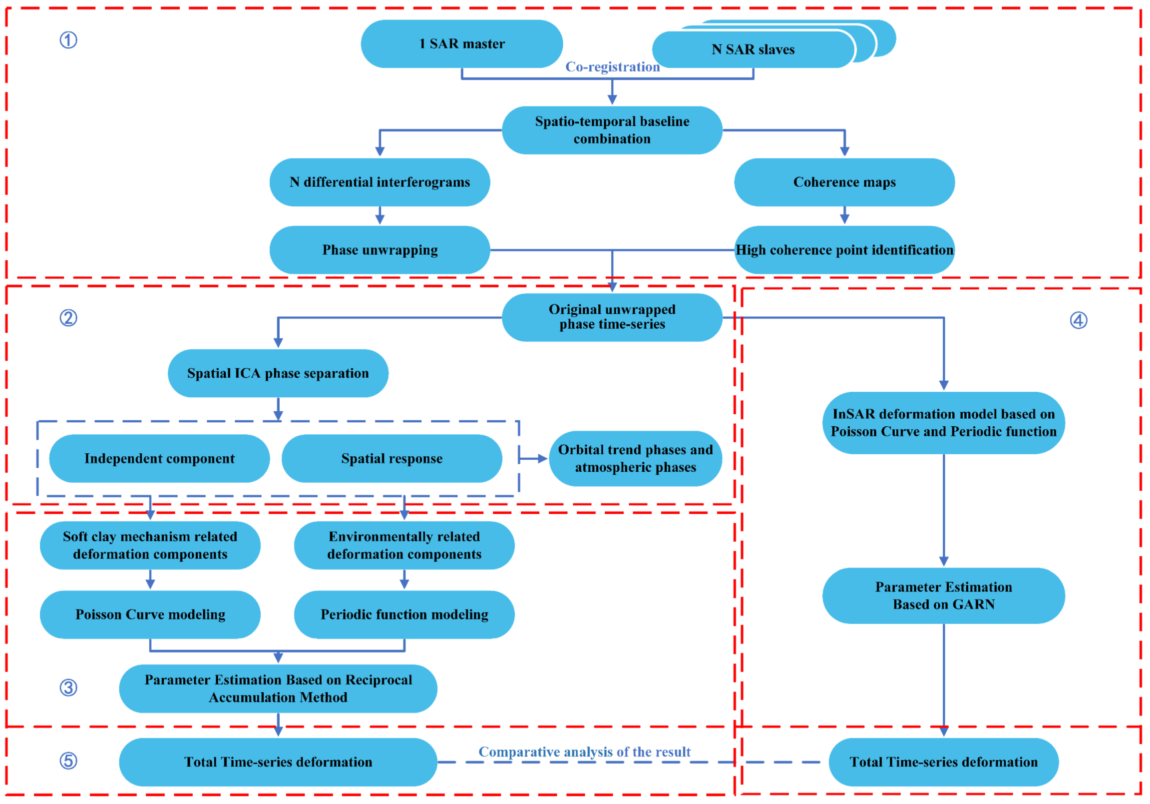
Figure 1 shows the flow chart of the FIPR algorithm. The key steps are as follows:
(1)
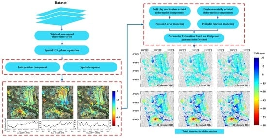
Unwrapped phase time series of differential interferometry are generated using the SBAS technique;
(2)
Spatial ICA phase separation based on FastICA: generating the spatial independent component and temporal response of each component;
(3)
Deformation modeling and parameter estimation: Deformation modeling for the extracted soft clay-related components with Poisson function and the environmental-related components with periodical functions; model parameters estimation using the reciprocal accumulation method, and generating the time series of each defor-mation component based on the estimated parameters;
(4)
Deformation generation using the GARN algorithm and traditional equal-weighted accumulation modeling;
(5)
Comparison and analysis of the total time-series deformation generated by the FIPR algorithm and the traditional equal-weighted accumulation modeling algorithm.

3. Simulated Experiment

To verify the effect of ICA on the separation of deformation phases and guide the real data experiments, a simulation experiment was designed and executed here. Two groups (six images for each group) of temporal deformation fields were simulated based on the Poisson function represented as (7) and the periodical function represented as (8) with a region of 100   ×   100 pixel area. The linear orbital error components were modeled with a linear trend mathematical function z = j x + k y + c , where j and k are random numbers following a normal distribution. The satellite parameters used here were set according to the images acquired in the real data experiment (TerraSAR X-band, Stripmap descending). After superimposing the three simulated original signals, two independent groups of experiments were conducted with temporal ICA (tICA) and spatial ICA (sICA) processing. Figure 2 shows partial results using sICA and tICA separation. It is clearly seen from the figure that the sICA separation fits better with the original signals compared to tICA.
To quantitatively evaluate the accuracy of the two groups of results, the RMSE (root mean square error) between the extracted deformation components and the simulated real values was calculated for each temporal acquisition. Figure 3 shows the sICA-separated results including the spatial responses (top) and time series (middle) for the two related deformation components, and the comparison between the RMSE of tICA (the length of each blue histogram) and sICA (the length of each top red histogram) generated results. The spatial response was normalized to −1 to 1. The overall RMSE of the Poisson-related components obtained by sICA was estimated as less than 2 mm, which was significantly lower than tICA, which had an RMSE higher than 6 mm. The maximum improvement for sICA was 85.8% at day 120. Similarly, for the periodical deformation components, the effect of sICA was still greatly improved, with an overall RMSE of 3 mm and a 22.3% improvement compared with that of tICA. This indicated that for the Poisson deformation signals, the sICA-separated results were much closer to the original signals than that of tICA. Since the high coherence points in the acquired InSAR dataset were spatially densely distributed but temporally sparsely discontinuous, sICA performed better for the signal separation than tICA [27]. Consequently, the spatial ICA algorithm is more recommended for our subsequent real data experiments.

4. Real Data Experiments

4.1. Study Area and Data Processing

The experimental area selected in this paper was around the Beijing Capital Airport. The soil in this area is mainly soft clay. The capital airport is the largest aviation port in China, and from 1978 to 2018, the annual passenger throughput of the Beijing Capital International Airport expanded from 1.03 to 110 million, ranking 1st in Asia and 2nd in the world. Figure 4 shows the geographic location of the study area. The capital airport is located in a flat area (within the elevation range of 22.0–35.4 m) between the alluvial fan of the Wenyu River and the Chaobai River, with a complex geological environment and partially crossing poor geological areas, such as lotus ponds and fish ponds. According to our in situ investigation and consultation of the reference geological materials, it was learned that the geological components of the roadbed were mostly newly deposited clayey and sandy soils [38,39,40]. Under the combined influence of natural and human activities, the equilibrium of the airport surface was highly susceptible to subsidence and disruption, which requires necessary long-term stability monitoring. A total of 24 TerraSAR-X-band Stripmap ascending images (track number 157), from 22 January 2012 to 6 February 2015, were collected and utilized. All the SAR interferometry processing was conducted via GAMMA software, and 23 high-quality unwrapped interferometric pairs were finally selected and generated for the subsequent processing [41].

4.2. InSAR Phase-Independent Component Analysis

As discussed in Section 3, the sICA algorithm was utilized in the real data experiments to conduct the independent phase component separation. For the specific implementation, to determine the appropriate number of independent components for our experiments, the contribution rates for each group of experiments under the specific number of components were calculated in advance. It was shown that for the five independent components, the cumulative contribution rate could reach 88%, indicating that when the number was greater than five, the remaining contribution of components occupied less than 12%, which could be ignored. The contribution of the first five independent components was defined according to the ratio value defined by Liu et al. [23], which were estimated as 8.56, 5.14, 8.25, 7.08, and 6.70, orderly. The smaller the ratio value, the greater the contribution of the corresponding independent component. Consequently, the number of independent components was set as five in our experiment. Figure 5 shows the obtained spatial response (top) and temporal response (bottom) of the five independent components (ICs) via the FastICA algorithm (the spatial response was normalized from −1 to 1). From Figure 5 we can see that for IC1 and IC3 there are no obvious spatial correlation characteristics in the spatial response image (top-left) and no significant variation pattern in the time-series response curve, inferring that the IC1 and IC3 signal may be related to the residual orbital error and partly topography-related tropospheric delay effects. For IC2 and IC5, the overall spatial response of most points in regions A and B showed a similar linear displacement trend, which was suggested to be related to the long-term deformation displacement, as their time-series responses showed an “S” shaped trend, reflecting a high dependence on time. Areas A and B were two typical subsiding areas, which will be further analyzed.
In Figure 5 we can also see that the IC4 signal showed an obvious periodic variation (as shown in the bottom-left of the figure); therefore, it is suggested as the environment-related deformation component. To reveal the correlation between the periodic deformation component and the precipitation, we conducted a correlation analysis between the extracted periodic deformation component and the precipitation in the area, which is shown in Figure 6. In the figure we can see that an obvious correlation with a 5-month lag effect was revealed. The average correlation coefficient between the periodic deformation component and precipitation was estimated as 0.536 and can be improved to 0.761 after the correction of the five-month lag.

4.3. Analysis of the Generated Total Time-Series Deformation via FIPR

Figure 7 shows the generated total time-series deformation results from 22 January 2012 to 6 February 2015 obtained via the FIPR algorithm. From the spatial color distribution, we can see that two obvious subsidence funnels were detected: the Jinzhan area (area A) and the northwest of the capital airport (area B), which are also revealed in Figure 5 (the enlarged image of A and B at the bottom-right of Figure 5). The area of Jinzhan mainly presented a color pattern of red-orange to crimson, and the overall average settlement over the area accumulated to 45 mm, with a maximum settlement of 126 mm on 6 February 2015. In contrast, the settlement in the northwestern part of the airport was significantly weaker, mainly orange-yellow, with overall average subsidence of higher than 40 mm and a maximum subsidence of 62 mm. The Jinzhan area suffered the most obvious ground subsidence in the Beijing plain, where the subsidence was suggested as mainly related to serious groundwater exploitation over the area. The development of ground settlement was easily induced by excessive groundwater exploitation, where the change in groundwater level accelerated the surface settlement [42]. In contrast, the degree of groundwater exploitation in the northwestern area of the capital airport was relatively weak, inducing a relatively stable phenomenon of surface deformation compared with the Jinzhan area. Judging from the temporal change in the color pattern over the area, the overall area stayed stable from 22 January to 20 September 2012, while from 20 September to 18 September 2013, the deformation increased under a gradually increased subsiding velocity; from 18 September 2013 to 6 February 2015, the deformation rate generally followed a trend from gradually decreasing to stable, which is consistent with the nonlinear subsiding law of soft clay consolidation disciplines.

4.4. Accuracy Analysis

To verify the accuracy of our proposed FIPR algorithm, first, we conducted a correlation analysis between the FIPR-generated time-series deformation results and the elevation of groundwater level at each monitoring well for groundwater pumping. The correlation and consistency between the deformation and the groundwater level depths can reflect the accuracy of the generated subsidence. Figure 8 shows the results of the average subsidence rate obtained via the FIPR algorithm, which was used as a background image to show the locations of six feature points near the monitoring wells (see P1–P6 in Figure 8 for the location of the feature points), where the feature points P1–P3 are located in the subsidence funnel of Jinzhan district (area A), and P4–P6 are located in the subsidence funnel of the northwest of the capital airport (area B). The pressurized groundwater measurements for the six monitoring wells within the subsidence funnels are drawn in Figure 9 and Figure 10 (the purple dashed lines) and compared with the deformation results generated via traditional EWA-LM (linear model with equal weight accumulation) and EWA-PC (Poisson curve with equal weight accumulation). It is clear from the subfigures in Figure 9 and Figure 10 that the blue line shows the best consistency with the purple dashed line (which denotes the underground water level) compared with the red and the green lines. This indicates that the FIPR-generated results showed the best accuracy. To quantitatively represent the correlation between the obtained deformation results at each feature point and the groundwater level, we calculated the exact correlation coefficients, which are shown in Table 1. The results indicated that the FIPR-generated deformations showed the best correlation coefficient, estimated as 0.946, whereas the maximum coefficient of EWA-LM and EWA-PC were 0.793 and 0.907, respectively. The reason for this phenomenon is suggested to be related to the artificial uncertainty in modeling induced by artificial assumptions for different physical deformation components via EWA-LM and EWA-PC. The uncertainty can be removed by the ICA technique and can be referenced in revising the weights of different deformation components in EWA-LM and EWA-PC.
To verify the modeling accuracy of FIPR, the magnitude of the high-pass (HP) deformation component was utilized here. According to [43], the HP deformation component can characterize the modeling accuracy of the deformation models. The smaller the HP deformation component, the higher the modeling accuracy. The HP deformation of each interferogram obtained through the FIPR was compared with those of EWA-PC and EWA-LM. Figure 11 shows a comparison of the HP deformation over all the high coherence points for each interferogram. As shown in Figure 11, for all the interferograms, the root mean square (RMS) of the HP deformation generated by the FIPR was estimated as ±2.6 mm, less than that of the EWA-LM, indicating that the FIPR was more suitable for the time-series deformation in the test area. The RMS of the HP deformation was estimated as ±4.1 mm for EWA-LM and ±3.1 mm for EWA-PC. The accuracy of FIPR was an improvement of 36.6% compared to that of EWA-LM and 16.1% compared to that of EWA-PC.
In addition, we also collected the ground leveling measurements at three benchmarks in the test area to evaluate the external accuracy of our proposed algorithm. The locations of the three benchmarks are shown in Figure 8 (G1, G2, and G3), which are mainly distributed around the Capital International Airport. The temporal span of the leveling measurements was from September 2012 to September 2013. To conduct an accurate comparison, we transferred the generated line of sight (LOS) deformation into vertical displacement according to the equation S LOS = S v cos θ and extracted the six dates of the measurements, which spanned periods consistent with the obtained SAR acquisitions. The comparison results are shown in Figure 12. As seen in the figure, the FIPR showed the best consistency with the leveling measurements. The bottom-left corner of Figure 12 shows the quantitative comparison results of the RMSE on the benchmarks. According to our calculation, the RMSE of FIPR was estimated as ±1.0 mm; compared with that of EWA-PC, the accuracy was improved by 50%, while the RMSE of EWA-PC was ±3.3 mm, with an improvement of 69.7%.

5. Discussions

5.1. Potential Reasons for the Derived Deformation

According to previous studies [44,45], the extent and rate of ground subsidence in the Beijing plain area were directly related to groundwater overexploitation. The pore elastic response of the soft clay layer to groundwater extraction acts as an elastic recoverable settlement or an inelastic, permanent compression-induced surface deformation. When the aquifer system exhibits continuous compression associated with a declining groundwater table, recoverable permanent subsidence of the soft clay layer occurs. As shown in Figure 8, the Jinzhan area (area A in Figure 5) is the most obvious subsiding area in the Beijing plain. Groundwater in the Jinzhan area is mainly endowed with the loose pore medium of the quaternary system, with fine particles of quaternary sediments and a large thickness of compressible layers. The quaternary system contains plentiful layers of pore aquifers, including both sand and gravel layers with coarser particles and good water-richness, and the clay layers with finer particles and higher compressibility, which were formed under the alluvial and flooding effects of the Yongding River and Chaobai River. The deposition environment is considerably complex. Affected by tectonic activities and the intensity of groundwater exploitation, the ground subsidence in the Jinzhan area maintains a serious level all year and is highly related to the variations in groundwater levels. Using the collected Beijing Water Resources Bulletin data from 2012 to 2015 provided by the Beijing Municipal Water Bureau [46], we obtained the overall depth of the groundwater level in the Capital International Airport area and compared it with the extracted time-series subsidence at the feature points (P1–P6 in Figure 8) for a detailed analysis. As shown in Figure 10, the time-series variations of groundwater level and the FIPR-derived subsidence of the feature points showed good consistency. When the groundwater level decreased from groundwater overexploitation, the voids between soil particles were compressed under an external constant load; thus, the deformation at this stage (before 2014) was characterized by a fast sinking rate; from July 2014, the natural compression of the soil layer reached its limit and the pore ratio decreased to a constant lowest value, causing the groundwater level to be stable. Consequently, the deformation was characterized by a decreasing subsiding velocity and tended to be stable afterward.
For other areas around the capital airport, the ground deformation was also mainly related to the underground responses of the soft clay with groundwater exploitation. As shown in Figure 10, we can see that from 2012 to 2013, the buried depth of the groundwater level in the capital airport area decreased significantly with reference to the beginning of the year, followed by a slight increase. The ground surface of the capital airport area remained stable during this stage; in contrast, in 2013, the serious over-extraction of groundwater led to a 1.5 m drop in the groundwater level, which induced serious surface subsidence of a maximum of 60 mm around the capital airport. At the end of 2014, water resources were sufficient in Beijing during the “South-to-North Water Diversion” project, which mitigated water use and groundwater exploitation in Beijing, and accordingly, the groundwater level tended to slowly stabilize. Consequently, the ground surface settlement maintained a stable status at this time.
In addition to the abovementioned effects of anthropogenic groundwater extraction, another geological-related reason was suggested here. From Figure 8 we can see that there is a clear linear boundary in the northwestern part of the capital airport (marked as a red dotted line), which is a potential correlation between the surface subsidence and the underground geological faults. According to [45], the Shunyi-Liangxiang fault was drawn with a red dashed line in Figure 8, located in the airport area. The Shunyi-Liangxiang fault crosses the entire airport and divides it into two parts with obviously different subsidence rates. To reveal the subsidence characteristics for the two different areas of the airport quantitively, a cross-section of the airport runway (marked as F-F′) was extracted and shown in Figure 13. From the figure, we can see that the Northwest part of the airport showed relatively serious subsidence with a maximum rate of 50 mm/yr, whereas the Eastern part had a relatively uniform and stable rate of lower than 10 mm/yr. The clearly different subsiding rates on both sides of the fault indicated that it was still active, and its location may impose a significant impact on the spatial distribution of ground subsidence. Therefore, close and continuous long-term subsidence monitoring of the airport runway in this area will provide an important reference for safety operations.

5.2. Applicability Analysis for ICA

(1)
FastICA was used to separate the original InSAR signals to extract the exact component of each physical deformation signal based on each independent component, which can help to accurately determine the exact weight of each deformation signal related to different physical factors. The exact weight (or certain contribution of each component) can be utilized to guide subsequent deformation modeling, which can greatly reduce the uncertainty of artificial equal weight modeling assumptions. The results showed that the accuracy was significantly improved compared to the traditional InSAR equal weight modeling;
(2)
The number of independent components (ICs) played an important role in ICA-based time-series InSAR analysis. Both too high and too low numbers of ICs will limit the accuracy of signal extraction. The number of ICs was mostly obtained through empirical and experimental calculations. The ideal number of ICs in this study was set as five, which was determined by experiments with different samples of numbers of ICs;
(3)
In this paper, spatial ICA was more reliable than temporal ICA. The main reason was that the spatial independence of the deformation signal was better than the temporal independence in the study area, as revealed by the spatial–temporal expanding characteristics of the two subsiding funnels shown in Figure 7. As shown, during the monitoring period, the area of subsidence in areas A and B gradually expanded from 1.9 and 2.3 km2 to 12.3 and 9.6 km2, respectively, with clear independent subsiding boundaries; in contrast, according to our temporal correlation analysis, the correlation coefficient between the Poisson-related deformation component and the environment-related component was 0.43, indicating that the two signals were not independent (still showing a high correlation and not perfectly separated temporally). Therefore, spatial ICA separation was suggested here to produce a better time-series deformation signal related to different physical causes.

6. Conclusions

A time-series InSAR deformation estimation algorithm, namely, FIPR (FastICA Poisson-curve reciprocal accumulation method), was proposed in this paper. Each deformation component was extracted through the FIPR from the original InSAR unwrapped phase signals based on FastICA, and each extracted component was modeled based on its physical characteristics. The Poisson curve was utilized to model the soft soil-related physical deformation component, and the reciprocal accumulation method (RAM) was introduced to estimate the model parameters to generate the total time-series deformation.
Both simulated and real data experiments were designed and conducted. The simulated experimental results indicated that the sICA-separated signals were much closer to the original than those of tICA, with the RMSE lower than 2 mm, and accordingly were more highly recommended. In the real data experiment, the area around Beijing Capital International Airport in China was selected as the study area. With the use of 24 high-resolution TerraSAR-X radar satellite images, the deformation sequences from January 2012 to February 2015 were obtained with a maximum cumulative subsidence of 126 mm. The spatial–temporal evolution characteristics of the deformation were analyzed. Two obvious subsidence funnels were detected, where the Jinzhan region suffered the most obvious subsidence, with an accumulated settlement of up to 126 mm. The reason for the subsidence was suggested as related to serious overexploitation of the groundwater.
To evaluate the accuracy of the proposed algorithm, the RMS of HP deformations and the RMSE from the external leveling measurements were estimated. The accuracy of the proposed model was estimated as ±2.6 mm, with an improvement of 36.6% compared to that of the EWA-LM (linear model with equal weight accumulation) algorithm and 16.1% compared to the EWA-PC (Poisson-curve with equal weight accumulation) algorithm. The RMSE from external leveling measurements was estimated as ±1.0 mm, with 69.7% improvement compared to EWA-LM and 50% to EWA-PC. It can be inferred that RAM can avoid the disadvantages of traditional GA and improve the accuracy and efficiency of calculation. FIPR can reduce the uncertainty of artificial assumptions in deformation modeling and improve the accuracy of deformation analysis for soft clay areas, also providing a reference for road maintenance and traffic safety management.

7. Patents

There are patents resulting from the work reported in this manuscript. We have applied for a Chinese patent (202110368285.4) entitled “A monitoring method of soft clay deformation using time-series InSAR technology.”

Author Contributions

Conceptualization, X.X. and L.Z.; methodology, X.X. and B.L.; software, X.M. and B.L.; validation, W.P. and L.Z.; formal analysis, X.X. and L.Z.; investigation, X.X.; resources, B.L. and X.M.; data curation, X.M.; writing—original draft preparation, L.Z. and X.M.; writing—review and editing, X.X., W.P. and R.Z.; visualization, W.P.; supervision, X.X.; project administration, X.X.; funding acquisition, X.X.,W.P. and R.Z. All authors have read and agreed to the published version of the manuscript.

Funding

This work was supported by the National Natural Science Foundation of China (No. 42074033, 41701536, 61701047, 41674040, 41904003), the Natural Science Foundation of Hunan Province (No. 2022JJ30589, 2017JJ3322, 2019JJ50639), Hunan International Scientific and Technological Innovation Cooperation Base of Advanced Construction and Maintenance Technology of Highway (Changsha University of Science and Technology) (kfj190805).

Acknowledgments

The TerraSAR dataset used in this study was provided by the DLR (Deutsches Zentrum für Luftund Raumfahrt, No. MTH3393, MTH3728).

Conflicts of Interest

The authors declare no conflict of interest.

References

  1. Lin, H.; Ma, P.F.; Wang, W.X. Urban Infrastructure Health Monitoring with Spaceborne Multi-temporal Synthetic Aperture Radar Interferometry. Acta Geo. Cartogr. Sin. 2017, 46, 1421–1433. [Google Scholar]
  2. Pan, W.Q. Monitoring and analysis of ground settlement during pipe roof construction of pipe-jacking groups in soft soil areas. Chin. J. Geotech. Eng. 2019, 41, 201–204. [Google Scholar]
  3. Xing, X.M.; Chang, H.C.; Chen, L.F.; Zhang, J.H.; Yuan, Z.H.; Shi, Z.N. Radar Interferometry Time Series to Investigate Deformation of Soft Clay Subgrade Settlement—A Case Study of Lungui Highway, China. Remote Sens. 2019, 11, 429. [Google Scholar] [CrossRef]
  4. Yu, J.; Sun, M.; He, S.; Huang, X.; Wu, X.; Liu, L. Accumulative Deformation Characteristics and Microstructure of Saturated Soft Clay under Cross-River Subway Loading. Materials 2021, 14, 537. [Google Scholar] [CrossRef] [PubMed]
  5. Ferretti, A.; Prati, C.; Rocca, F. Permanent scatterers in SAR interferometry. IEEE Trans. Geosci. Remote Sens. 2001, 39, 8–20. [Google Scholar] [CrossRef]
  6. Berardino, P.; Fornaro, G.; Lanari, R.; Sansosti, E. A new algorithm for surface deformation monitoring based on small baseline differential SAR interferograms. IEEE Trans. Geosci. Remote Sens. 2002, 40, 2375–2383. [Google Scholar] [CrossRef]
  7. Luo, Q.; Zhou, G.; Perissin, D. Monitoring of Subsidence along Jingjin Inter-City Railway with High-Resolution TerraSAR-X MT-InSAR Analysis. Remote Sens. 2017, 9, 717. [Google Scholar] [CrossRef]
  8. Qin, X.Q.; Yang, M.S.; Wang, H.M.; Yang, T.L.; Lin, J.X.; Liao, M.S. Application of High-resolution PS-InSAR in Deformation Characteristics Probe of Urban Rail Transit. Acta Geo. Cartogr. Sin. 2016, 45, 713–721. [Google Scholar]
  9. Fan, H.D.; Gao, X.X.; Yang, J.K.; Deng, K.Z.; Yu, Y. Monitoring mining subsidence using a combination of phase-stacking and offset-tracking methods. Remote Sens. 2015, 7, 9166–9183. [Google Scholar] [CrossRef]
  10. Qin, X.Q.; Liao, M.S.; Zhang, L.; Yang, M.S. Structural health and stability assessment of high-speed railways via thermal dilation mapping with time-series InSAR analysis. IEEE J. Sel. Top. Appl. Earth Obs. Remote Sens. 2017, 10, 2999–3010. [Google Scholar] [CrossRef]
  11. Qin, X.Q.; Zhang, L.; Yang, M.S.; Luo, H.; Liao, M.S.; Ding, X.L. Mapping surface deformation and thermal dilation of arch bridges by structure-driven multi-temporal DInSAR analysis. Remote Sens. Environ. 2018, 216, 71–90. [Google Scholar] [CrossRef]
  12. Chen, B.B.; Gong, H.L.; Chen, Y.; Lei, K.C.; Zhou, C.F.; Si, Y.; Li, X.J.; Pan, Y.; Gao, M.M. Investigating land subsidence and its causes along Beijing high-speed railway using multi-platform InSAR and a maximum entropy model. Int. J. Appl Earth Obs. Geoinf. 2021, 96, 102284. [Google Scholar] [CrossRef]
  13. Wang, R.; Yang, T.L.; Yang, M.S.; Liao, M.S.; Lin, J.X. A safety analysis of elevated highways in Shanghai linked to dynamic load using long-term time-series of InSAR stacks. Remote Sens Lett. 2019, 10, 1133–1142. [Google Scholar] [CrossRef]
  14. Li, S.S.; Li, Z.W.; Hu, J.; Sun, Q.; Yu, X.Y. Investigation of the Seasonal oscillation of the permafrost over Qinghai-Tibet Plateau with SBAS-InSAR algorithm. Chin. J. Geophys. 2013, 56, 1476–1486. [Google Scholar]
  15. Zhang, Y.H.; Wu, H.A.; Sun, G.T. Deformation Model of Time Series Interferometric SAR Techniques. Acta Geo. Cartogr. Sin. 2012, 41, 864–869. [Google Scholar]
  16. Zhu, L.J.; Xing, X.M.; Zhu, Y.K.; Peng, W.; Yuan, Z.H.; Xia, Q. An advanced time-series InSAR approach based on poisson curve for soft clay highway deformation monitoring. IEEE J. Sel. Top. Appl. Earth Obs. Remote Sens. 2021, 14, 7682–7698. [Google Scholar] [CrossRef]
  17. Hoyer, P.O.; Hyvärinen, A. Independent component analysis applied to feature extraction from colour and stereo images. Netw. Comput. Neural Syst. 2000, 11, 191. [Google Scholar] [CrossRef]
  18. De, L.E.; De, M.S.; Falanga, M.; Palo, M.; Notes, A. Decomposition of high-frequency seismic wavefield of the Strombolian-like explosions at Erebus volcano by independent component analysis. Geophys. J. Int. 2009, 177, 1399–1406. [Google Scholar]
  19. Besic, N.; Vasile, G.; Chanussot, J.; Stankovic, S. Polarimetric incoherent target decomposition by means of independent component analysis. IEEE Trans. Geosci. Remote Sens. 2014, 53, 1236–1247. [Google Scholar] [CrossRef]
  20. Forootan, E.; Kusche, J. Separation of global time-variable gravity signals into maximally independent components. J. Geod. 2012, 86, 477–497. [Google Scholar] [CrossRef]
  21. Dai, W.J.; Huang, D.W.; Cai, C.S. Multipath mitigation via component analysis methods for GPS dynamic deformation monitoring. GPS Solut. 2014, 18, 417–428. [Google Scholar] [CrossRef]
  22. Wen, H.J.; Huang, Z.W.; Wang, Y.L.; Liu, H.L.; Zhu, G.B. Application of Independent Component Analysis in GRACE-Derived Water Storage Changes Interpretation: A Case Study of the Tibetan Plateau and Its Surrounding Areas; Springer: Cham, Switzerland, 2015; pp. 179–188. [Google Scholar]
  23. Liu, B.; Dai, W.J.; Liu, N. Extracting seasonal deformations of the Nepal Himalaya region from vertical GPS position time series using independent component analysis. Adv. Space Res. 2017, 60, 2910–2917. [Google Scholar] [CrossRef]
  24. Luo, F.X.; Dai, W.J.; Tang, C.P.; Huang, D.W.; Wu, X.X. EMD-ICA with Reference Signal Method and Its Application in GPS Multipath. Acta Geo. Cartogr. Sin. 2021, 41, 366–371. [Google Scholar]
  25. Ballatore, P. Extracting digital elevation models from SAR data through independent component analysis. Int. J. Remote Sens. 2011, 32, 3807–3817. [Google Scholar] [CrossRef]
  26. Ebmeier, S.K.; Biggs, J.; Mather, T.A.; Amelung, F. Applicability of InSAR to Tropical Volcanoes: Insights from Central America. Geological Society; Special Publications: London, UK, 2013; Volume 380, pp. 15–37. [Google Scholar]
  27. Gaddes, M.E.; Hooper, A.; Bagnardi, M.; Inman, H.; Albino, F. Blind signal separation methods for InSAR: The potential to automatically detect and monitor signals of volcanic deformation. J. Geophys. Res. Solid Earth. 2018, 123, 10226–10251. [Google Scholar] [CrossRef]
  28. Peng, M.M.; Lu, Z.; Zhao, C.Y.; Motagh, M.; Lin, B.; Conway, B.D.; Chen, H.Y. Mapping land subsidence and aquifer system properties of the Willcox Basin, Arizona, from InSAR observations and independent component analysis. Remote Sens. Environ. 2022, 271, 112894. [Google Scholar] [CrossRef]
  29. Jutten, C.; Herault, J. Blind separation of sources, Part I: An adaptive algorithm based on neuromimetic architecture. Signal Process. 1991, 24, 1–10. [Google Scholar] [CrossRef]
  30. Zhu, K.; Zhang, X.; Sun, Q.; Wang, H.; Hu, J. Characterizing Spatiotemporal Patterns of Land Deformation in the Santa Ana Basin, Los Angeles, from InSAR Time Series and Independent Component Analysis. Remote Sens. 2022, 14, 2624. [Google Scholar] [CrossRef]
  31. Stone, J.V. Independent component analysis: An introduction. Trends Cogn. Sci. 2002, 6, 59–64. [Google Scholar] [CrossRef]
  32. Maubant, L.; Pathier, E.; Daout, S.; Radiguet, M.; Doin, M.-P.; Kazachkina, E.; Kostoglodov, V.; Cotte, N.; Walpersdorf, A. Independent Component Analysis and Parametric Approach for Source Separation in InSAR Time Series at Regional Scale: Application to the 2017–2018 Slow Slip Event in Guerrero (Mexico). J. Geophys. Res. Solid Earth. 2020, 125, e2019JB018187. [Google Scholar] [CrossRef]
  33. Hyvarinen, A. Fast and robust fixed-point algorithms for independent component analysis. IEEE Trans. Neural Netw. 1999, 10, 626–634. [Google Scholar] [CrossRef] [PubMed]
  34. Hyvärinen, A.; Oja, E. Independent component analysis: Algorithms and applications. Neural Netw. 2000, 13, 411–430. [Google Scholar] [CrossRef]
  35. Ma, X.J.; Liu, B.; Dai, W.J.; Kuang, C.L.; Xing, X.M. Potential Contributors to Common Mode Error in Array GPS Displacement Fields in Taiwan Island. Remote Sens. 2021, 13, 4221. [Google Scholar] [CrossRef]
  36. Ge, R.Y.; Wang, Y.B.; Zhang, J.P.; Yao, L.; Zhang, H.; Long, Z.Y. Improved FastICA algorithm in fMRI data analysis using the sparsity property of the sources. J. Neurosci. Meth. 2016, 263, 103–114. [Google Scholar] [CrossRef] [PubMed]
  37. Zai, J.M.; Mei, G.X. Forecast method of settlement during the complete process of construction and operation. Rock. Soil Mech. 2000, 21, 322–325. [Google Scholar]
  38. Chen, B.B.; Gong, H.L.; Lei, K.C.; Li, J.W.; Zhou, C.F.; Gao, M.L.; Guan, H.L.; Lv, W. Land subsidence lagging quantification in the main exploration aquifer layers in Beijing plain, China. Int. J. Appl. Earth Obs. Geoinf. 2019, 75, 54–67. [Google Scholar] [CrossRef]
  39. Chen, M.; Tomás, R.; Li, Z.H.; Motagh, M.; Li, T.; Hu, L.Y.; Gong, H.Y.; Li, X.J.; Yu, J.; Gong, X.L. Imaging land subsidence induced by groundwater extraction in Beijing (China) using satellite radar interferometry. Remote Sens. 2016, 8, 468. [Google Scholar] [CrossRef]
  40. Gao, M.L.; Gong, H.L.; Chen, B.B.; Zhou, C.F.; Chen, W.F.; Liang, Y.E.; Shi, M.; Si, Y. InSAR time-series investigation of long-term ground displacement at Beijing Capital International Airport, China. Tectonophysics 2016, 691, 271–281. [Google Scholar] [CrossRef]
  41. Costantini, M.; Rosen, P.A. A Generalized Phase Unwrapping Approach for Sparse Data. In Proceedings of the International Geoscience and Remote Sensing Symposium, Hamburg, Germany, 28 June–2 July 1999; pp. 267–269. [Google Scholar]
  42. Chen, B.B.; Gong, H.L.; Li, X.J.; Lei, K.C.; Zhu, L.; Gao, M.L.; Zhou, C.F. Characterization and causes of land subsidence in Beijing, China. Int. J. Remote Sens. 2017, 38, 808–826. [Google Scholar] [CrossRef]
  43. Zhao, R.; Li, Z.W.; Feng, G.C.; Wang, Q.J.; Hu, J. Monitoring surface deformation over permafrost with an improved SBAS-InSAR algorithm: With emphasis on climatic factors modeling. Remote Sens. Environ. 2016, 184, 276–287. [Google Scholar] [CrossRef]
  44. Zhou, C.F.; Gong, H.L.; Chen, B.B.; Zhu, F.; Duan, G.Y.; Gao, M.L.; Lu, W. Land subsidence under different land use in the eastern Beijing plain, China 2005–2013 revealed by InSAR timeseries analysis. GISci. Remote Sens. 2016, 53, 671–688. [Google Scholar] [CrossRef]
  45. Gao, M.L.; Gong, H.L.; Li, X.J.; Chen, B.B.; Zhou, C.F.; Shi, M.; Lin, G.; Chen, Z.; Ni, Z.Y.; Duan, G.Y. Land subsidence and ground fissures in Beijing capital international airport (bcia): Evidence from quasi-ps insar analysis. Remote Sens. 2019, 11, 1466. [Google Scholar] [CrossRef] [Green Version]
  46. Beijing Water Authority. Available online: http://swj.beijing.gov.cn (accessed on 11 December 2021).
Figure 1. Flow chart of the FIPR algorithm.
Remotesensing 14 04253 g001
Figure 2. Comparison of the separated results of tICA and sICA at each temporal date (left: Poisson-related components; right: periodical deformation components).
Remotesensing 14 04253 g002
Figure 3. ICA separated results (top-left: spatial response of Poisson-related components, and top-right: spatial response of periodic deformation components; middle-left: time series of Poisson-related components and middle-right: time series of periodic deformation components; bottom-left: comparison of tICA and sICA-separated results of Poisson-related components at each temporal point; bottom-right: comparison of tICA and sICA separation results of periodic deformation components at each temporal point (the length of each blue histogram represents the RMSE value of tICA, whereas the top red one represents that of sICA).
Remotesensing 14 04253 g003
Figure 4. The geographic location of the study area.
Remotesensing 14 04253 g004
Figure 5. The spatial–temporal response of each independent component (top: spatial response of each independent component; bottom: time series of each independent component; Areas A and B were two typical subsiding areas.).
Remotesensing 14 04253 g005
Figure 6. Correlation analysis between the periodic deformation components and precipitation.
Remotesensing 14 04253 g006
Figure 7. Time-series deformation results over the study area (with reference to 22 January 2012; Areas A and B were two typical subsiding areas.).
Remotesensing 14 04253 g007
Figure 8. Locations of the ground-monitoring wells and ground benchmarks with the mean velocity map as background (Areas A and B were two typical subsiding areas; F-F′ is Shunyi-Liangxiang fault; G1–G3 is the position of three benchmarks; P1–P6 represent six feature points.).
Remotesensing 14 04253 g008
Figure 9. Correlation analysis between the time-series deformation results and the elevations of groundwater level (EWA-LM: linear model with equal weight accumulation; EWA-PC: Poisson curve with equal weight accumulation; UWL: elevation of groundwater level) at (a): P1; (b): P2; (c): P3.
Remotesensing 14 04253 g009
Figure 10. Correlation analysis between the time-series deformation results and the elevations of groundwater level (EWA-LM: linear model with equal weight accumulation; EWA-PC: Poisson curve with equal weight accumulation; UWL: elevation of groundwater level) (a): P4; (b): P5; (c): P6.
Remotesensing 14 04253 g010
Figure 11. RMS of HP deformation comparison of 23 SAR images (EWA-LM: linear model with equal weight accumulation; EWA-PC: Poisson curve with equal weight accumulation).
Remotesensing 14 04253 g011
Figure 12. Time-series deformation results compared with leveling measurements on benchmarks. (a) G1 in Figure 8. (b) G2. (c) G3.
Remotesensing 14 04253 g012
Figure 13. Cross-section analysis along F-F′ in Figure 8.
Remotesensing 14 04253 g013
Table 1. Correlation coefficients between the deformation obtained by the three methods and the groundwater level.
PointsEWA-LMEWA-PCFIPR
P10.7750.8100.898
P20.7930.8350.895
P30.7840.7580.871
P40.7790.8180.932
P50.7770.9070.937
P60.7860.8020.946
Publisher’s Note: MDPI stays neutral with regard to jurisdictional claims in published maps and institutional affiliations.

