Technical Note

An Efficient MUSIC Algorithm Enhanced by Iteratively Estimating Signal Subspace and Its Applications in Spatial Colored Noise

National Key Laboratory of Radar Signal Processing, Xidian University, Xi’an 710071, China
*
Author to whom correspondence should be addressed.
Remote Sens. 2022, 14(17), 4260; https://doi.org/10.3390/rs14174260
Submission received: 4 July 2022 / Revised: 9 August 2022 / Accepted: 24 August 2022 / Published: 29 August 2022

Abstract

:
The classical multiple signal classification (MUSIC) algorithms mainly have two limitations. One is an insufficient number of snapshots, which usually causes an ill-posed sample covariance matrix in many real applications. The other limitation is the intense space-colored and time-white noise, which also breaks the separability between signal and noise subspaces. In the case of the insufficient sample, there are few signal components in the non-zero delay sample covariance matrix (SCM), where the space-colored and time-white noise components are suppressed by the temporal method. A set of non-zero delay sample covariance matrices are constructed, and a nonlinear object function is formulated. Hence, the sufficient non-zero delay SCMs ensure that enough signal components are used for signal subspace estimation. Then, the constrained optimization problem is converted into an unconstrained one by exploiting the Lagrange multiplier method. The nonlinear equation is solved by Newton’s method iteratively. Moreover, a proper initial value of the new algorithm is given, which can improve the convergence of the iterative algorithm. In this paper, the noise subspace is removed by the pre-projection technique in every iteration step. Then, an improved signal subspace is obtained, and a more efficient MUSIC algorithm is proposed. Experimental results show that the proposed algorithm achieves significantly better performance than the existing methods.

1. Introduction

Spatial spectrum estimation is an important research field in array signal processing [1,2,3,4,5,6,7,8,9,10,11,12,13,14,15,16,17,18,19,20,21,22,23,24,25,26,27,28,29,30,31,32,33,34,35,36,37,38,39,40,41,42,43,44,45,46,47,48,49,50,51,52,53]. In the past few decades, spatial spectrum estimation has been widely used in radar, wireless communication, sonar, hyperspectral image processing [54,55], and many other areas [2,3,5]. The core of this technique is to estimate the parameters of targets [5,6,7,8,9].
The spatial spectrum of the MUSIC algorithm has high resolution [1,4]. Usually, the MUSIC algorithm [1] estimates the subspace by eigenvalue decomposition (EVD) of a single sample covariance (correlation) matrix [1,3,5,10,30]. Meanwhile, the uniformity or consistency of the smallest eigenvalues is used to determine the dimension and select the basis vectors of the noise subspace. One of the key elements of MUSIC is the orthogonality between signal and noise subspaces, which is used to design the spatial spectrum function [1,3,5]. Then, the function peaks are determined by scanning multiple local maximum points with suitable step sizes, and the locations of the peaks correspond to the direction of arrival (DOA) [1,2,3,5,6,8,13,18,20]. It can be seen that the performance of the classical MUSIC algorithm depends heavily on the accuracy of the estimated subspace [1,2,5].
The signal subspace is spanned by the eigenvectors associated with the largest eigenvalues of the sample covariance matrix (SCM), and its dimension should be equal to the number of targets [5,8,9,10]. Similarly, the noise subspace is formulated by the eigenvectors associated with the smallest eigenvalues of the SCM. If insufficient snapshots are received, the SCM will be deficiently estimated, and the uniformity of all the corresponding smallest eigenvalues will be broken, resulting in significant performance degradation of the relative algorithms [2,3,6,9,21,23,40].
In recent years, machine learning (ML) and deep learning (DL) have received considerable attraction [5,6,8,10]. ML and DL adopt learning-based and data-driven architectures, which can learn the non-linear relationship between input and output data. DOA estimation via DL is considered in [5], where a multilayer perception (MLP) architecture is proposed to deal with two target signals. In [6], the authors study the same problem by exploiting the sparsity of the received signal in the angular domain and designing a deep convolutional neural network (CNN). A single target case is assumed in [8], and a cognitive radar scenario is considered, where DL is applied for sparse array selection and DOA estimation. However, the computational complexity of algorithms [5,6,8,10] dramatically increases with the number of targets.
Many DOA estimation algorithms [10,11,12,13,16,23,33,48,49,50,51,52] have been proposed in the corresponding period. In [10], the conjugate subspace is introduced into two-dimensional MUSIC (2D-MUSIC), and a half spatial spectrum search strategy is applied to reduce computation complexity, but the algorithm is only suitable for uncorrelated sources. In [9,20], the authors utilize compressive sensing and sparse representation [48,49,50,51,52] to resolve the two-dimensional DOA estimation problem. Several two-dimensional DOA estimation algorithms based on the L-shaped planar array (with a larger aperture) are proposed [12,19,20,25,32,33,35,36], which have low computational complexity. In [30], the auto-correlation and cross-correlation information is used, and an efficient algorithm is proposed to deal with the DOA estimation problem. In [31], the augmented covariance matrix is employed, and then the two-dimensional DOA estimation problem is converted into two one-dimensional estimation problems. In [13,24,25], a non-circular high-order singular value decomposition (HOSVD) algorithm is developed for DOA estimation. However, the computational complexity of the algorithm [13,24,25,48,49,50,51,52] is very high.
Initially, the design of the above algorithms [10,11,12,13,14,15,16,17,18,19,20,21,22,23,24,25] assumes that the space-colored and time-white noise is not present in observations. However, the received data vectors are sometimes contaminated by space-colored and time-white noise in real applications [48,49,50,51,52], such as radar and sonar. Hence, the performance of these algorithms [10,11,12,13,14,15,16,17,18,19,20,21,22,23,24,25] may be severely degraded in this case [34,36,37,38,39,40,41,42,43,44,45,46,47,48,49,50,51,52].
Several DOA estimation algorithms that can work in space-colored and time-white noise circumstances have been developed [37,38,39,40,41,42,43,44,45,46,47,48,49,50]. In [37], the authors formulate the DOA estimation problem as an off-grid sparse model and handle it by sparse Bayesian learning. The joint DOA and direction of departure (DOD) estimation method [38] is proposed, which can eliminate space-colored and time-white noise by three-transmitter configurations. The joint DOD and DOA estimation method is studied in [40], which utilizes the multi-dimension structure inherent in observations to eliminate the impact of space-colored and time-white noise. In [39], the interrelationship between the two one-dimensional estimating signal parameters via rotational invariance techniques (ESPRIT) is exploited to automatically obtain paired DOA and DOD estimation without decreasing the performance of angle estimation. These algorithms [36,38,39,43,44] use a non-zero delay SCM to handle angle estimation problems and perform well under spatial colored noise circumstances.
The space-colored and time-white noise can be eliminated by exploiting the uncorrelated temporal property [36,38,39,40,41,44]. Some signal components may be missing in one non-zero delay SCM, especially for an insufficient number of snapshots. Fortunately, in the non-zero delay SCM sets, the probability of missing a signal component is extremely small. Thus, a set of non-zero delay SCMs has been developed to obtain an accurate signal subspace. In this paper, the pre-projection technique is employed to remove the adverse effect of the pure noise subspace. Based on this, an efficient MUSIC algorithm with an accurate subspace is developed in this paper, and a suitable initial value is calculated for the new subspace estimation algorithm.
The rest of the paper is organized as follows. Problem formulation is presented in Section 2.1, where the classical MUSIC is overviewed, and in Section 2.2, the motivations of our work are introduced. Then, the iterative subspace estimation algorithm and an efficient MUSIC algorithm are formulated. Section 3 shows the experimental results. Section 4 gives the discussion of this paper. Section 4 concludes this paper.

2. Materials and Methods

2.1. Problem Formulation

Without losing generality, this paper considers a uniform linear array (ULA) composed of M omnidirectional antennas. There are P narrow-band far-field plane waves that impinge on the system with different DOAs. The received data vector at the l-th snapshot is represented as
x l = A ( θ ) s l + n l
where A = a 1 θ 1 , a 2 θ 2 , , a P θ P M × P , a p θ p M × 1 is the signal steering vector (SSV) of the p-th far-field point source, θ = θ 1 , θ 2 , , θ P are the DOAs of the targets, and T is the transpose operator. s l P × 1 is the transmitted source vector sequence, and n l M × 1 represents the space-colored and time-white noise vector sequence.
Usually, it is assumed that the space-colored and time-white noise vector sequences (at different snapshots) are complex and conform to Gaussian distribution. Moreover, n l M × 1 is equipped with zero-mean and unknown covariance C M × M .
E n l i n l j H = C i = j 0 i j
where E and H , respectively, denote the expectation operator and complex conjugate transpose operator.
Moreover, it is assumed that the source and noise vectors are mutually independent of each other. Then, the ideal covariance matrix of the received data vectors can be expanded into
R = E x l x l H = A R s A + C
where R s = E s l s l H P × P . In practice, the ideal covariance matrix is unavailable. Hence, many studies employ the sample covariance matrix instead of the expected covariance matrix to estimate signal and noise subspaces in most cases. The sample covariance matrix (SCM) is given by
R ^ = 1 L l = 1 L x l x l H
where L is the number of snapshots.
The eigenvalue decomposition (EVD) of R ^ is expressed as
R ^ = U Λ U H = U s Λ s U s H + U n Λ n U n H
where Λ = Λ s 0 0 Λ n = diag ( λ 1 , , λ M ) M × M consists of the eigenvalues of SCM that are arranged in descending order λ 1 λ 2 λ M 0 , and U = U s , U n M × M is the corresponding eigenvector matrix. The diagonal matrix Λ s = diag ( λ 1 , , λ P ) P × P is formed by the first P largest eigenvalues, and the diagonal matrix Λ n = diag ( λ P + 1 , , λ M ) M P × M P consists of the last M P smallest eigenvalues. Here, U s M × P is constructed by the eigenvectors associated with the first P largest eigenvalues, and U n M × M P is formed by the eigenvectors associated with the last M P smallest eigenvalues. Since R ^ is at least a positive semi-definition matrix, U s M × P and U n M × M P must be the unitary matrix. Thus, we have U s H U s = I P P × P , U s H U n = 0 P × ( M P ) , and U n H U n = I M P M P × M P , where I P is a P × P identity matrix.
Furthermore, if there is a significant difference between the first P largest eigenvalues and the last MP smallest eigenvalues, in the conventional additive white Gaussian noise case, the eigenvalues related to pure noise (eigenvalues related to signal) can be easily distinguished according to the obvious difference. Then, the noise subspace U n M × P (signal subspace U s M × P ) is obtained.
For example, the classical MUSIC algorithms assume that the first P largest eigenvalues and the last M P smallest eigenvalues are non-uniform and approximately uniform, respectively. In this desired case, the first P largest eigenvalues are associated with the signal power plus partial noise power. The last M P smallest eigenvalues are only associated with the pure noise power. Thus, the dimension M P of the noise subspace U n is determined by evaluating the uniformity of the eigenvalues (corresponding to pure noise), where the uniformity satisfies λ P + 1 = λ P + 2 = = λ M . Under such a case, the columns of U s M × P and U n M × M P represent the basis vectors of the signal and the noise subspaces, respectively. Correspondingly, the eigenvector matrix U s M × P and U n M × M P are called the signal and noise subspaces, respectively.
In real applications, there is a desired relation
a H θ U n 0
where a θ is the signal steering vector (SSV). The spatial spectrum scanning function of the MUSIC algorithm is given by
max θ P MUSIC θ = 1 a H θ U n U n H a θ
Interestingly, the first few largest peaks of P MUSIC θ are particularly sharp. Therefore, the MUSIC algorithm can achieve super-resolution in comparison with the beamforming technique.
Remark 1:
It can be seen from experiments that the DOA estimate almost equals the actual one if the estimated noise subspace is accurate enough. However, there are two limitations: insufficient snapshots and intense space-colored and time-white noise. Insufficient snapshots will lead to the ill-posed  R ^ and will make all the eigenvalues of  R ^ non-uniform. For this case, a clear difference between the first P largest eigenvalues and the last  M P smallest eigenvalues does not exist. Hence, it is challenging to divide the signal subspace and the noise subspace correctly. More seriously, strong space-colored noise will cause one or more eigenvalues of the first P largest ones only related to noise, while the eigenvalues related to the signal (plus noise) are presented in the M P last smallest ones. Therefore, the signal and the noise subspaces are overlapped and undivided. A method for estimating the signal subspace or noise subspace more accurately is urgently needed for MUSIC.

2.2. Proposed Algorithm

2.2.1. Enhanced MUSIC Algorithm

The main motivation for this work is twofold. On the one hand, in the ideal case, the complex vector sequences n l are spatial colored and conform to temporal-white Gaussian distribution with an unknown covariance matrix C = C ( 0 ) = E n l n l H 0   . However, the non-zero delay covariance matrix is C ( τ ) = E n ( l ) n ( l τ ) H = 0   τ 0 . The classical MUSIC algorithm uses R to estimate the subspace, which requires C = σ n 2 I M ( σ n 2 denotes the noise power), i.e., the separability between the signal and the noise subspaces. If A R s A is not a full-rank matrix, the smallest eigenvalues of R are uniform. However, if C is a common complex matrix, then the smallest eigenvalues of R are often non-uniform. Thus, the separability between the signal subspace and the noise subspace is broken, which significantly degrades the accuracy of the estimated signal subspace or the noise subspace. However, the non-zero delay covariance matrix is C ( τ ) = E n ( l ) n ( l τ ) H = 0   τ 0 , which indicates that a less negative impact of the noise component is imposed on the non-zero delay SCMs R ( k ) = E x l x l + k H . Hence, an improved subspace can be extracted from the non-zero delay SCMs.
On the other hand, experiments show that the signal components may be missing in a non-zero delay SCM, but the signal components always exist in the set of non-zero delay SCMs when the number of received samples is insufficient. Hence, a more accurate signal subspace can be obtained in this case by using the non-zero delay SCMs instead of only a non-zero delay SCM.
However, the expected non-zero delay SCM is also unavailable. Referring to relation (4), this paper uses the following non-zero delay SCM instead of the ideal non-zero delay SCM to obtain the subspace
R ^ k = 1 L k l = 1 L k x l x l + k H
R ^ k is also an autocorrelation matrix ( R ^ k = R ^ k ), if the samples are composed of stationary random processes. Hence, when k ≥ 0, only the non-zero delay SCMs need to be calculated.
The non-zero delay SCMs R ^ k are reformulated as
R ^ k A R ^ s k A H + C ^ k
In random theory, C ^ k M × M should be equal to the zero matrix. However, since only limited samples are used to construct R ^ k , C ^ k is not equal to the null matrix in practice. Let matrix U ¯ s M × P consist of the basis vectors of the signal subspace, and the matrix U ¯ n M × M P be formed by all the basis vectors of the noise subspace. Then, U ¯ s , U ¯ n U ¯ s , U ¯ n H = I M and A = U ¯ s T , where T P × P denotes a matrix with full rank. Let B k = U ¯ s H A R ^ s k A H U ¯ s P × P , C 1 ( k ) = U ¯ s H C ^ k U ¯ s P × P , C 2 k = U ¯ s H C ^ k U ¯ n H P × M P , C 3 k = U ¯ n H C ^ k U ¯ s M P × P , and C 4 ( k ) = U ¯ n H C ^ k U ¯ n M P × M P . Moreover, (9) can be further expressed as
R ^ ( k ) U ¯ s B ( k ) U ¯ s H + U ¯ s C 1 ( k ) U ¯ s H + U ¯ s C 2 ( k ) U ¯ n H + U ¯ C n 3 ( k ) U ¯ s H + U ¯ n C 4 ( k ) U ¯ n H           = U ¯ s ( B ( k ) + C 1 ( k ) ) U ¯ s H + U ¯ s C 2 ( k ) U ¯ n H + U ¯ C n 3 ( k ) U ¯ s H + U ¯ n C 4 ( k ) U ¯ n H
When some signal components of R ^ k do not exist, B k is not a full-rank matrix. To avoid this undesired situation, a fused matrix is defined in this paper:
R ¯ = k = 1 K R ^ ( k ) R ^ H ( k ) = k = 1 K ( U ¯ s ( B ( k ) + C 1 ( k ) ) ( B ( k ) + C 1 ( k ) ) H U ¯ s H + U ¯ s C 2 ( k ) C 2 H ( k ) U ¯ s H + U ¯ n C 4 ( k ) C 4 H ( k ) U ¯ n H + U ¯ C n 3 ( k ) C 3 H ( k ) U ¯ n H + U ¯ C n 3 ( k ) U ¯ s H ( B ( k ) + C 1 ( k ) ) H U ¯ s H + U ¯ s ( B ( k ) + C 1 ( k ) ) C 3 H ( k ) U ¯ n H + U ¯ n C 4 ( k ) C 2 H ( k ) U ¯ s H + U ¯ s C 2 ( k ) C 4 H ( k ) U ¯ n H )
Note that the above equation is derived based on U ¯ s H U ¯ n = 0 , U ¯ s H U ¯ s = I P , and U ¯ n H U ¯ n = I M P × M P . It can be seen from (10) and (11) that the presence of the second term on the right side may reduce the accuracy of the estimated signal subspace.
If E ¯ = U ¯ s , the pre-projection expression E ¯ H R ^ k E ¯ is written as
E ¯ H R ^ ( k ) E ¯ = E ¯ H ( U ¯ s ( B ( k ) + C 1 ( k ) ) U ¯ s H + U ¯ s C 2 ( k ) U ¯ n H + U ¯ C n 3 ( k ) U ¯ s H + U ¯ n C 4 ( k ) U ¯ n H ) E ¯ = U ¯ s H ( U ¯ s ( B ( k ) + C 1 ( k ) ) U ¯ s H + U ¯ s C 2 ( k ) U ¯ n H + U ¯ C n 3 ( k ) U ¯ s H + U ¯ n C 4 ( k ) U ¯ n H ) U ¯ s = U ¯ s H U ¯ s ( B ( k ) + C 1 ( k ) ) U ¯ s H U ¯ s + U ¯ s H U ¯ s C 2 ( k ) U ¯ n H U ¯ s + U ¯ s H U ¯ C n 3 ( k ) U ¯ s H U ¯ s + U ¯ s H U ¯ n C 4 ( k ) U ¯ n H U ¯ s = U ¯ s H U ¯ s ( B ( k ) + C 1 ( k ) ) U ¯ s H U ¯ s + U ¯ s H U ¯ s C 2 ( k ) 0 ( M P ) × P + 0 P × ( M P ) C 3 ( k ) U ¯ s H U ¯ s + 0 P × ( M P ) C 4 ( k ) 0 ( M P ) × P = C 1 ( k ) + B ( k )
The above expression shows that the pure noise part in (10) can be removed by such pre-projection.
Inspired by (12), this paper builds the following objective function to take full advantage of multiple non-zero delay SCMs and the pre-projection technique:
max J E = k = 1 K E H R ^ k E 2 s . t   E H E = I P
where E M × P is the signal subspace with full column rank, and it can be obtained by solving (13). Let tr represent the matrix trace operator. Then, the following unconstrained optimization relation can be deduced by using the Lagrange multiplier method:
J E , Λ ˜ = k = 1 K tr E H R ^ H k E E H R ^ k E   tr   E H E I P Λ ˜
where Λ ˜ is the Lagrange multiplier matrix. Let the gradient of J E , Λ ˜ with respect to E H be equal to zero, and we have the following characteristic equation:
k = 1 K R ^ H k E E H R ^ k + R ^ k E E H R ^ H k E E Λ ˜ = 0
It can be seen that it is difficult to obtain the analytical solution to the nonlinear Equation (15). Hence, (15) should be solved by the iterative formula:
k = 1 K R ^ k V n 1 V H n 1 R ^ H k + R ^ H k V n 1 V H n 1 R ^ k V n = V n Λ
where V n 1 is the result of the (n−1)-th iteration.
Fix V n 1 , and then Equation (16) describes an EVD of k = 1 K R ^ k V n 1 V H n 1 R ^ H k + R ^ H k V n 1 V H n 1 R ^ k . It is well known that Newton’s method approximately solves the stationary point at each step, as does our method (16).
Thus, the new iterative algorithm is proposed and described as follows.
Let V 0 = v 1 0 , v 2 0 , , v P 0 M × P denote the initial value of the new algorithm, where a proper initial matrix V 0 consists of the first P left singular vectors of R ˜ = R ^ 1 , , R ^ K . Without losing generality, the (n − 1)-th iteration is represented as
G = k = 1 K R ^ k V n 1 V H n 1 R ^ H k + R ^ H k V n 1 V H n 1 R ^ k
The eigenvalue decomposition of G is formulated as
G = U n Λ n U H n
where Λ n = diag λ 1 n , λ 2 n , , λ M n , λ 1 n λ 2 n λ M n 0 , and U n is the eigenvector matrix of G . V n is composed of the first P columns of U n , and it can be expressed as
V n = U : , 1 : P
Thus far, one iteration from V n 1 to V n has been completed. The iterative process can be repeated until the algorithm meets the convergence condition. This paper sets the threshold as ε   0 < ε < 1 . When V n V H n V n 1 V H n 1 F ε , the iteration terminates. Hence, the estimated signal subspace is expressed as V s = V n , and the spatial spectrum of the enhanced MUSIC algorithm can be given by
P PROPOSED θ = 1 a H V n V n H a = 1 a H ( I V s V s H ) a = 1 a H a a H V s V s H a
Algorithm 1 illustrates the details.
Algorithm 1: Efficient MUSIC
Input data: X = x 1 , x 2 , , x L , ε, P; Output data: θ 1 , θ 2 , , θ P
1: R ^ k = 1 L k l = 1 L k x l x l + k H , V 0 s v d R ^ 1 , , R ^ K , initial n = 1
2: G = k = 1 K R ^ k V n 1 V H n 1 R ^ H k + R ^ H k V n 1 V H n 1 R ^ k
3: G = U n Λ n U H n , and arrange the diagonal elements of Λ n in descending order.
4: V n = U : , 1 : P
5: If V n V H n V n 1 V H n 1 F ε , end loop; else, jump to step 2.
6: P PROPOSED θ = 1 a H V n V n H a , then the first few largest peaks of P PROPOSED θ are particularly sharp, and θ 1 , θ 2 , , θ P is obtained.

2.2.2. Computational Complexity

The computational load of the conventional MUSIC algorithm mainly consists of three parts: building the zero-delay SCM R ^ , estimating noise subspace, and scanning operators. Constructing R ^ requires M 2 L flops (a flop indicates a floating-point multiplication [1,10,15]). Calculating the noise subspace needs O M 3 + M 2 P flops, and scanning one direction needs 2 M + M 2 flops.
Similarly, the computational complexity of the new algorithm consists of three parts. Constructing non-zero delay SCMs needs M 2 k = 1 K L k = M 2 K 2 L K 1 2 flops, calculating the signal subspace requires 2 M 2 K P + O M 3 flops in a single iteration, and the remaining computational complexity is 2 M + M 2 (in one direction).
Since the number of targets is very small, the new and classical MUSIC algorithms have the same order of computational complexity. The new algorithm usually takes 3–5 iterations to reach the convergence threshold, and it can obtain a more accurate subspace and higher resolution at the cost of higher computational complexity. With the continuous improvement of modern computing power, the increased computational complexity of the new algorithm is acceptable, and the proposed algorithm can achieve better performance in the presence of spatial color noise.

3. Results

Twenty elements are uniformly distributed on the ULA, where the space of adjacent elements is a half wavelength. The noise is complex time-white Gaussian, where the covariance matrix C is a random matrix on each simulation. Ten non-zero delay sample covariance matrices are constructed in the simulation, and it is assumed that there are three targets with plane wave-fronts impinging on the system from 30 ° , 0 ° , and 50 ° , respectively. In the experiments, 100 independent runs are used to obtain each point of the curve. The performance of [50,51,52,54,55], MUSIC, and the proposed algorithm is shown in this section.

3.1. Experiment 1: Subspace Accuracy

The formulation of the signal subspace [1,3,5] is given by
U ˜ s = A A H A 1 2
where A C M × P is the array manifold matrix. The projection matrix of U ˜ s is expressed as P s = U ˜ s U ˜ s H . Similarly, the n -th independent simulation estimated signal subspace is denoted as V ^ n , and the corresponding projection matrix is represented as P ^ n = V ^ n V ^ n H . Hence, the accuracy of the signal subspace is expressed as
10 log 10 1 N n = 1 N P s P ^ n F 2
Figure 1 illustrates the accuracy of the signal subspace versus signal–noise ratio (SNR). It can be seen from Figure 1 that the proposed algorithm can improve the subspace accuracy up to 1dB when the number of snapshots is fixed at 40. The accuracy of the signal subspace versus snapshots is shown in Figure 2. Obviously, the curves of Figure 2 indicate that the proposed algorithm achieves better performance than the conventional one, and it increases the accuracy by around 1dB when the input SNR is −10dB. It also can be seen that the subspace accuracy of the proposed algorithm is the same as that of the conventional algorithm at the lowest (the highest) input SNR. The most important and meaningful observation is that the proposed algorithm can achieve better performance at a moderate input SNR, and many systems work in this case. Two factors lead to this result. One factor is that the proposed algorithm employs sufficient non-zero delay SCMs estimating the subspace, while the conventional algorithm only uses an SCM (which is contaminated by spatial colored noise) to calculate the subspace. The other factor is that the pre-projection technique is introduced in the new algorithm.

3.2. Experiment 2: The Number of Iterations of the Proposed Algorithm

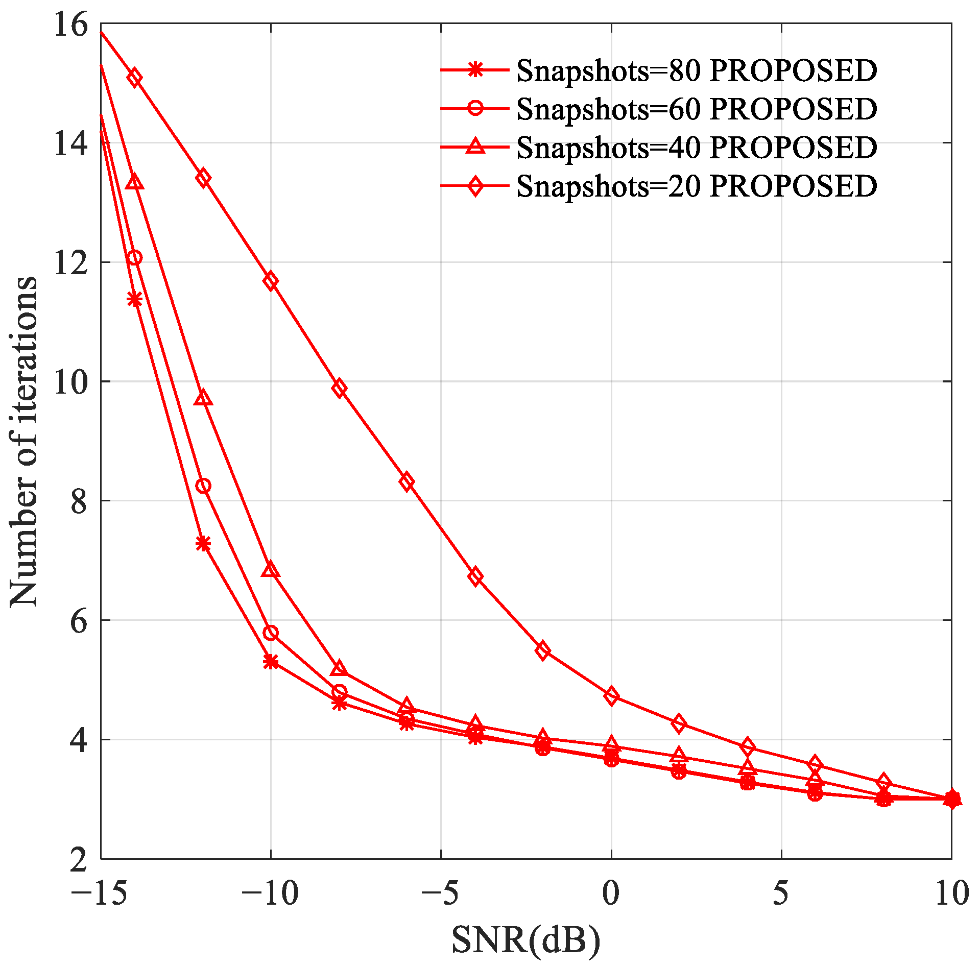
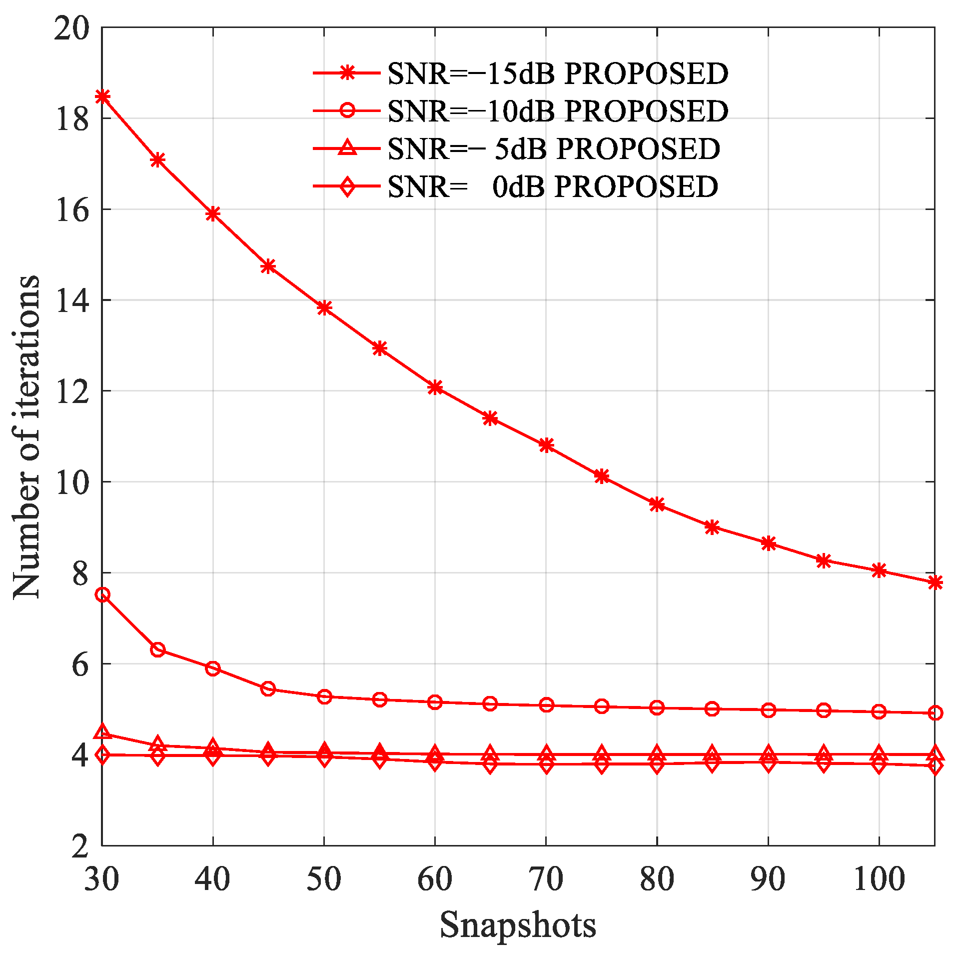
Figure 3 shows the number of iterations versus the input SNR, where the number of snapshots is set as 40. The number of iterations versus the number of snapshots is illustrated in Figure 4, where the input SNR is fixed at −10dB. It can be seen from Figure 3 and Figure 4 that the new algorithm needs more iterations to reach the convergence condition in the low input SNR region. In this experiment, 100 independent runs are performed to obtain each point of the curve, so the number of iterations is not an integer. Interestingly, the proposed algorithm only takes a few steps to meet the iteration end condition in most cases. Moreover, the noise level of many radar systems is from −15 dB to 10 dB. Overall, the new algorithm only takes a few steps to meet the final iteration in most cases.

3.3. Experiment 3: Root Mean Square Error

The root mean square error (RMSE) is given by
10 log 10 p = 1 P 1 P 1 N n = 1 N θ ^ p n θ p 2
where N = 100 represents the number of independent trials; P = 3 denotes the number of targets; θ p is the actual DOA of the p-th far-field target; θ ^ p n is the n-th estimated DOA of the p-th far-field target.
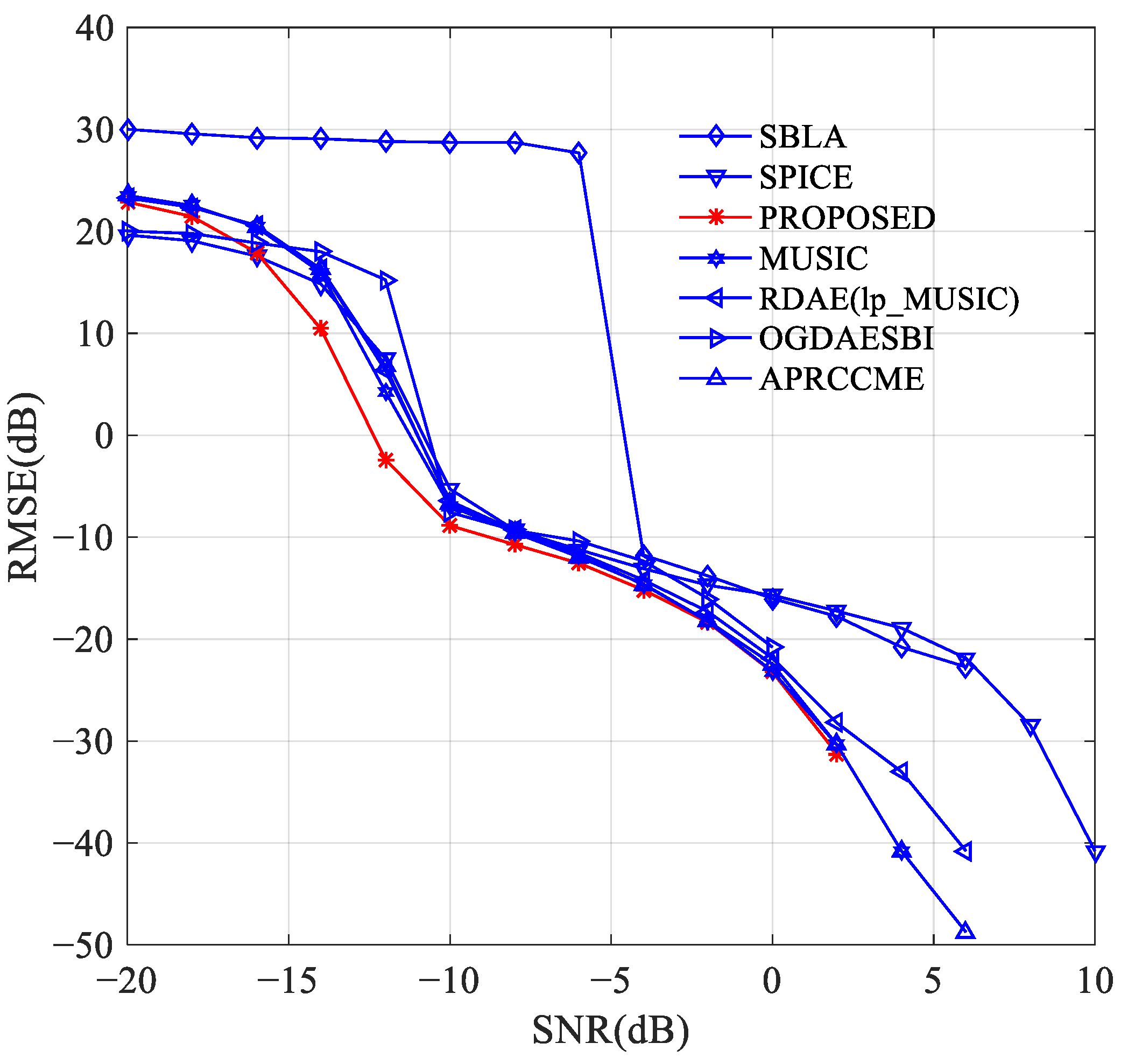
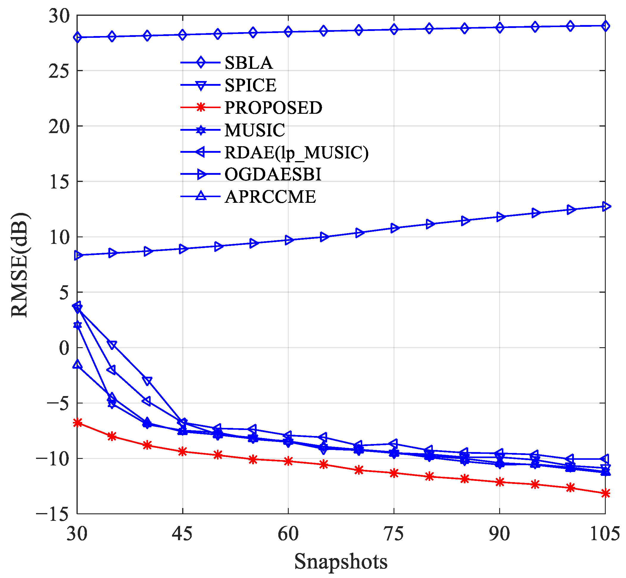
Figure 5 shows the RMSE versus the input SNR, where the number of the snapshots is fixed at 40. Figure 6 exhibits the RMSE versus the number of snapshots, where SNR = −10dB.
It can be seen from Figure 5 and Figure 6 that our algorithm outperforms the conventional MUSIC algorithm, the algorithms proposed in 50, 51, and other existing algorithms. The classical SBLA method fails to work, and the performance of the MUSIC algorithm and other existing algorithms degrades severely under the case of spatial colored and temporal-white Gaussian noise.
By contrast, our algorithm gives higher resolution and is more robust against the spatial colored and temporal-white Gaussian noise. The reason that the MUSIC, SPICE, and other existing algorithms have a low resolution is that they do not consider the spatial colored and temporal-white Gaussian noise.
The sparse Bayesian algorithm does not need prior knowledge such as the number of sources and does not require a few snapshots.
However, the RMSE is heavily dependent on the size of the overcomplete basis vectors. Moreover, these algorithms have lower computational efficiency than subspace-based algorithms because they use time-consuming nonlinear iterative steps. The RMSE of the proposed algorithm is superior to that of MUSIC owing to its better subspace.
In addition, the spatial colored noise significantly impacts the performance of the Bayesian algorithm.

3.4. Experiment 4: Spatial Spectrum

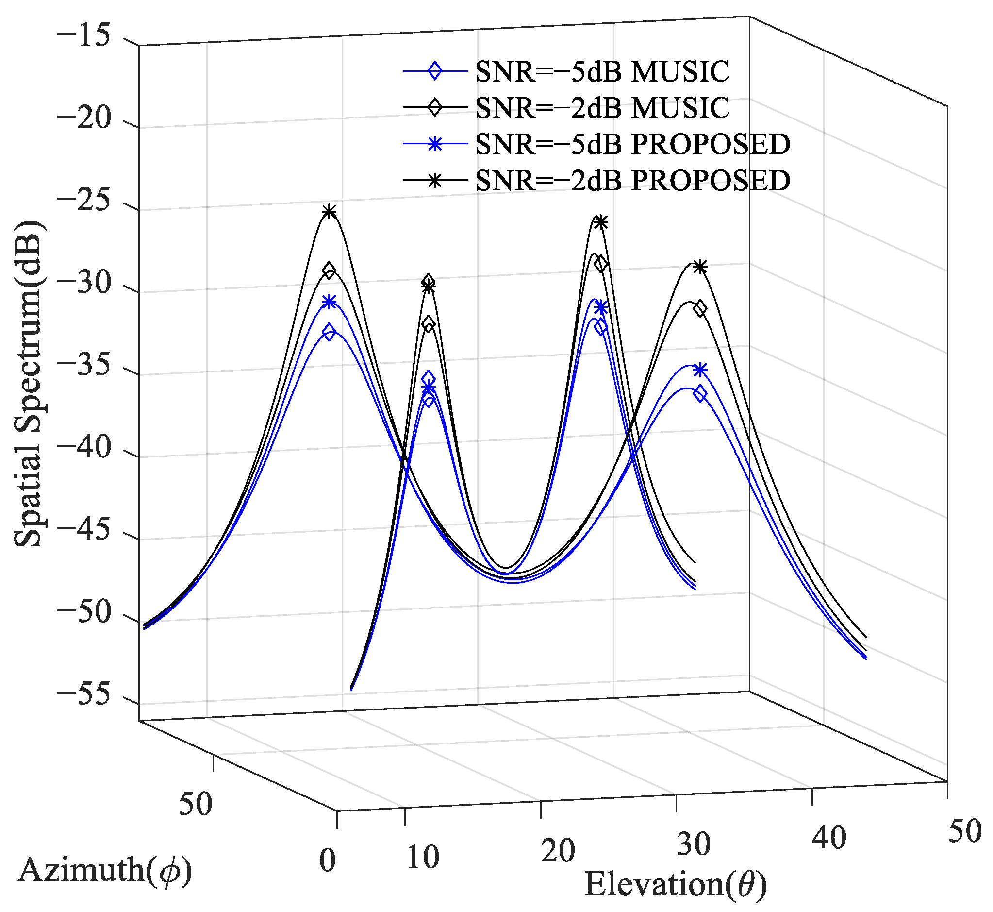
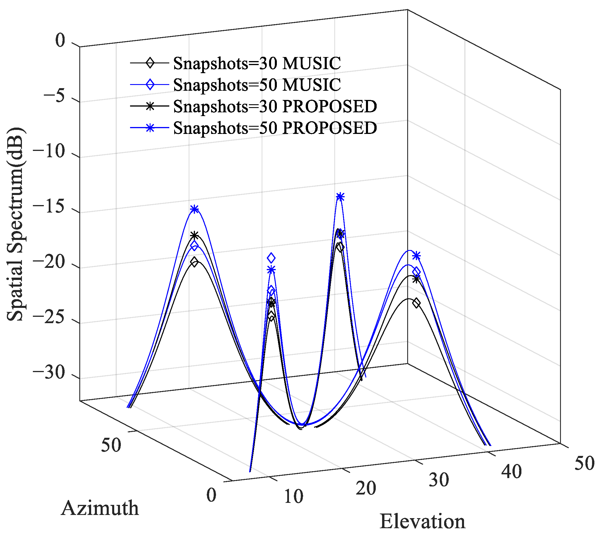
Twelve elements are uniformly distributed on the outer circular array, where the radius is 0.9 of the wavelength. Another six sensors are equally located in the inner circular array, where the radius is 0.5 of the wavelength. This study constructs 10 non-zero delay sample covariance matrices. In the first three experiments, 100 independent runs are performed to obtain each point. It is assumed that four targets with plane wave-fronts impinge on the system from (18°, 15°), (58°, 15°), (18°, 35°), and (58°, 35°), respectively.
Figure 7 shows the spatial spectra of both algorithms at different input SNRs, where the number of snapshots is 30. Figure 8 shows the spatial spectra at different snapshots when the input is −5dB. It can be seen from Figure 7 and Figure 8 that the estimated spatial spectra of the new algorithm are higher than those of the conventional MUSIC algorithm under the same circumstance. The proposed algorithm has a higher resolution than the classical MUSIC algorithm.

3.5. Experiment 5: Probabilities of Successful Discrimination (PSD)

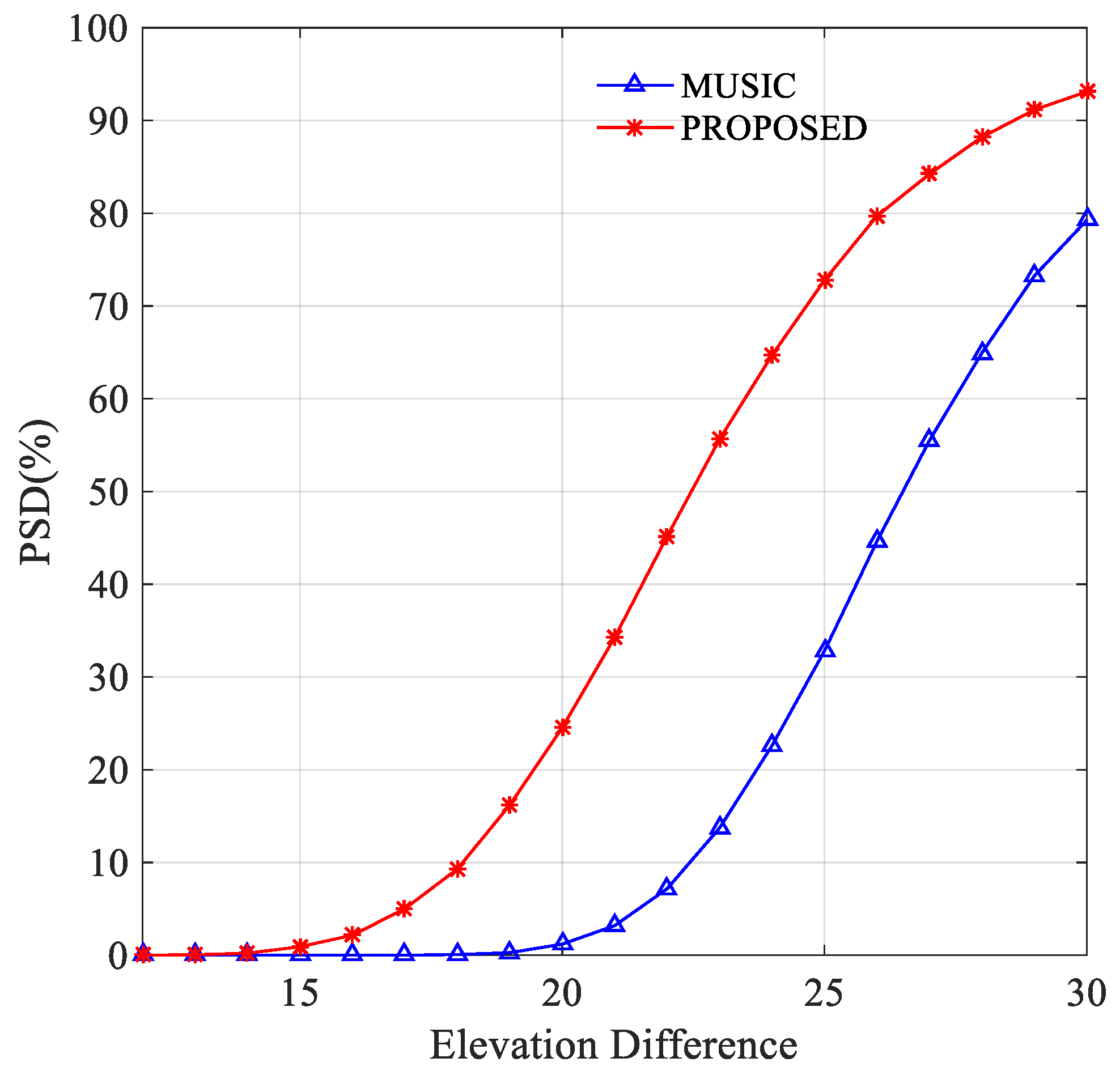
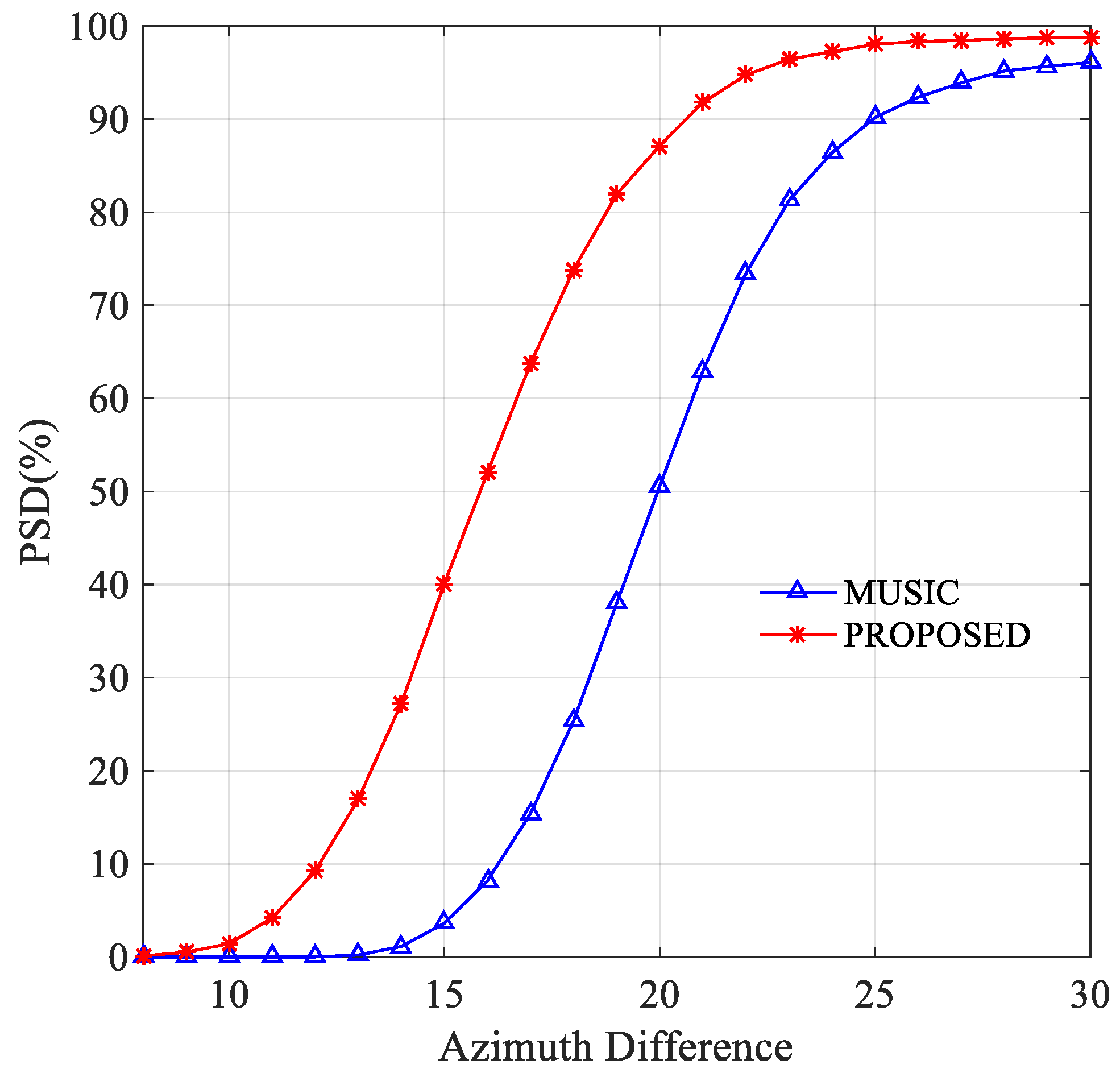
In the first case, the elevation is fixed at 30 ° , and the azimuth difference between the two targets is gradually increased. In the second case, the azimuth at 100 ° is specified, and the elevation difference of both targets is continuously expanded. Since the step size is set at 1 ° , when the error is less than 2 ° , successful discrimination is obtained (the configuration of the experiment is the same as that in Experiment 4).
Figure 9 and Figure 10 show the PSD of the new and conventional MUSIC algorithms. It can be seen that the resolution of the proposed algorithm is superior to that of the conventional algorithm.

4. Conclusions

This paper proposes a novel MUSIC algorithm with iterative subspace estimation for angle estimation. The design of the proposed algorithm considers the uncorrelated temporal property of space-colored and time-white noise, and a series of non-zero delay SCMs are constructed. Meanwhile, to remove residual noise, the pre-projection technique is introduced into the proposed algorithm. Then, an efficient non-linear objective function is formulated, and an iterative subspace estimation algorithm is deduced. Experimental results show that the proposed MUSIC algorithm achieves higher subspace estimation accuracy than the classical MUSIC algorithm. Moreover, it has a higher resolution and lower RMSE than the existing DOA estimation algorithms.

Author Contributions

Conceptualization, X.Z.; Funding acquisition, D.F.; Methodology, X.Z. and D.F; Supervision, D.F.; Writing—original draft, X.Z.; Writing—review and editing, X.Z. and D.F. All authors have read and agreed to the published version of the manuscript.

Funding

This work was supported by the National Natural Science Foundation of China under Grants 61971470 and 61971349.

Data Availability Statement

Not applicable.

Conflicts of Interest

The authors declare no conflict of interest.

References

  1. Wen, F.; Wan, Q.; Fan, R.; Wei, H. Improved MUSIC Algorithm for Multiple Noncoherent Subarrays. IEEE Signal Process. Lett. 2014, 21, 527–530. [Google Scholar] [CrossRef]
  2. Rao, B.D.; Hari, K.V.S. Performance analysis of ESPRIT and TAM in determining the direction of arrival of plane waves in noise. IEEE Signal Proc. Lett. 1989, 40, 1990–1995. [Google Scholar] [CrossRef]
  3. Nie, W.-K.; Feng, D.-Z.; Xie, H. Improved MUSIC algorithm for high resolution angle estimation. Signal Process. 2016, 122, 87–92. [Google Scholar] [CrossRef]
  4. Wang, B.; Zhao, Y.P.; Liu, J.J. Mixed-Order MUSIC Algorithm for Localizations in of Far-Field and Near-Field Sources. IEEE Signal Process. Lett. 2013, 20, 311–314. [Google Scholar] [CrossRef]
  5. Liu, Z.-M.; Zhang, C.; Yu, P.S. Direction-of-Arrival Estimation Based on Deep Neural Networks With Robustness to Array Imperfections. IEEE Trans. Antennas Propag. 2018, 66, 7315–7327. [Google Scholar] [CrossRef]
  6. Wu, L.-L.; Liu, Z.-M.; Huang, Z.-T. Deep Convolution Network for Direction of Arrival Estimation With Sparse Prior. IEEE Signal Process. Lett. 2019, 26, 1688–1692. [Google Scholar] [CrossRef]
  7. Huang, H.; Peng, Y.; Yang, J.; Xia, W.; Gui, G. Fast Beamforming Design via Deep Learning. IEEE Trans. Veh. Technol. 2020, 69, 1065–1069. [Google Scholar] [CrossRef]
  8. Wang, Y.; Liu, M.; Yang, J. Data-Driven Deep Learning for Automatic Modulation Recognition in Cognitive Radios. IEEE Trans. Veh. Technol. 2019, 68, 4074–4077. [Google Scholar] [CrossRef]
  9. Elbir, M.; Mishra, K.V. Joint antenna selection and hybrid beamformer design using unquantized and quantized deep learning networks. IEEE Trans. Wirel Commun. 2020, 19, 1677–1688. [Google Scholar] [CrossRef]
  10. Yu, X.Y.; Guo, Y. Efficient 2D-DOA estimation algorithm for multi-FH signals. J. Syst. Eng. Electron. 2018, 465, 180–187. [Google Scholar]
  11. Luo, J.; Zhang, Y.; Yang, J.; Zhang, D. Online Sparse DOA Estimation Based on Sub–Aperture Recursive LASSO for TDM–MIMO Radar. Remote Sens. 2022, 14, 2133. [Google Scholar] [CrossRef]
  12. Hua, Y.; Sarkar, T.K.; Weiner, D.D. An L-shaped array for estimating 2-D directions of wave arrival. IEEE Trans. Antennas Propag. 1991, 39, 143–146. [Google Scholar] [CrossRef]
  13. Yang, B.; Huang, D.; Liu, S. 2D-DOA estimation for uniform rectangular array using non-circular HOSVD method. In Proceedings of the 2016 11th International Symposium on Antennas, Propagation and EM Theory (ISAPE), GuiLin, China, 18–22 October 2016; pp. 617–620. [Google Scholar]
  14. Liu, L.; Rao, Z. An Adaptive Lp Norm Minimization Algorithm for Direction of Arrival Estimation. Remote Sens. 2022, 14, 766. [Google Scholar] [CrossRef]
  15. Lan, X.; Li, Y.; Wang, E. A RARE Algorithm for 2D DOA Estimation Based on Nested Array in Massive MIMO System. IEEE Access 2016, 4, 3806–3814. [Google Scholar] [CrossRef]
  16. Hua, Y. Estimating two-dimensional frequencies by matrix enhancement and matrix pencil. IEEE Trans. Signal Process. 1992, 40, 2267–2280. [Google Scholar] [CrossRef]
  17. Rouquette, S.; Najim, M. Estimation of frequencies and damping factors by two-dimensional ESPRIT type methods. IEEE Trans. Signal Process. 2000, 49, 237–245. [Google Scholar] [CrossRef]
  18. Chen, F.-J.; Fung, C.C.; Kok, C. Estimation of Two-Dimensional Frequencies Using Modified Matrix Pencil Method. IEEE Trans. Signal Process. 2007, 55, 718–724. [Google Scholar] [CrossRef]
  19. Dong, Y.-Y. 2-D DOA Estimation for L-Shaped Array With Array Aperture and Snapshots Extension Techniques. IEEE Signal Process. Lett. 2017, 24, 495–499. [Google Scholar] [CrossRef]
  20. Tayem, N.; Majeed, K.; Hussain, A.A. Two-Dimensional DOA Estimation Using Cross-Correlation Matrix With L-Shaped Array. IEEE Antennas Wirel. Propag. Lett. 2016, 15, 1077–1080. [Google Scholar] [CrossRef]
  21. Xu, L.; Wu, R.H.; Zhang, X.F. Joint Two-Dimensional DOA and Frequency Estimation for L-Shaped Array via Compressed Sensing PARAFAC Method. IEEE Access 2018, 6, 37204–37213. [Google Scholar] [CrossRef]
  22. Zhang, G.; Xie, J.; Zhang, H.; Li, Z.; Qi, C. Dynamic Antenna Selection for Collocated MIMO Radar. Remote Sens. 2022, 14, 2912. [Google Scholar] [CrossRef]
  23. Hu, W. DOA Estimation for UCA in the Presence of Gain-Phase Errors. IEEE Wirel. Commun. Lett. 2019, 23, 446–449. [Google Scholar] [CrossRef]
  24. Ahmed, T.; Zhang, X.; Hassan, W.U. A Higher-Order Propagator Method for 2D-DOA Estimation in Massive MIMO Systems. IEEE Commun. Lett. 2020, 24, 543–547. [Google Scholar] [CrossRef]
  25. Xia, T.-Q. Joint diagonalization based 2D-DOD and 2D-DOA estimation for bistatic MIMO radar. Signal Process. 2015, 116, 7–12. [Google Scholar] [CrossRef]
  26. Chintagunta, S.; Ponnusamy, P. 2D-DOD and 2D-DOA estimation using the electromagnetic vector sensors. Signal Process. 2018, 147, 163–172. [Google Scholar] [CrossRef]
  27. Xu, K.-J.; Nie, W.-K.; Feng, D. A multi-direction virtual array transformation algorithm for 2D DOA estimation. Signal Process. 2016, 125, 122–133. [Google Scholar] [CrossRef]
  28. Xu, S.Z.; Kooij, B.J.; Yarovoy, A. Joint Doppler and DOA estimation using (Ultra-)Wideband FMCW signals. Signal Process. 2020, 168, 107259. [Google Scholar] [CrossRef]
  29. Qiang, X.W.; Liu, Y.; Feng, Q.X. Adaptive DOA estimation with low complexity for wideband signals of massive MIMO systems. Signal Process. 2020, 176, 107702. [Google Scholar] [CrossRef]
  30. Dai, X.; Zhang, X.; Wang, Y. Extended DOA-Matrix Method for DOA Estimation via Two Parallel Linear Arrays. IEEE Commun. Lett. 2019, 23, 1981–1984. [Google Scholar] [CrossRef]
  31. Zheng, Z.; Mu, S. Two-Dimensional DOA Estimation Using Two Parallel Nested Arrays. IEEE Commun. Lett. 2020, 24, 568–571. [Google Scholar] [CrossRef]
  32. Chen, H.; Liu, Y.; Wang, Q. Two-Dimensional Angular Parameter Estimation for Noncircular Incoherently Distributed Sources Based on an L-Shaped Array. IEEE Sens. J. 2020, 20, 13704–13715. [Google Scholar] [CrossRef]
  33. Li, Z.; Zhang, X.; Shen, J. 2D-DOA Estimation of Strictly Non-circular Sources Utilizing Connection-Matrix for L-Shaped Array. IEEE Wirel. Commun. Lett. 2021, 10, 296–300. [Google Scholar] [CrossRef]
  34. Chen, P.; Cao, Z.X.; Chen, Z.M. Sparse off-grid DOA estimation method with unknown mutual coupling effect. Digit. Signal Process. 2019, 90, 1–9. [Google Scholar] [CrossRef]
  35. Guldogan, M.B.; Arikan, O. Cross-ambiguity function domain multipath channel parameter estimation. Digit. Signal Process. 2012, 22, 275–287. [Google Scholar] [CrossRef]
  36. Liang, J.L.; Liu, D. Joint estimation of source number and DOA using simulated annealing algorithm. Digit. Signal Process. 2010, 20, 887–899. [Google Scholar] [CrossRef]
  37. Yuan, J.; Zhang, G.; Liu, W.; Wang, X. Off-grid sparse DOA estimation based iterative reweighted linear interpolation in spatial coloured noise. Electron. Lett. 2020, 56, 573–575. [Google Scholar] [CrossRef]
  38. Jin, M.; Liao, G.S.; Li, J. Joint DOD and DOA estimation for bistatic MIMO radar. Signal Process. 2009, 89, 244–251. [Google Scholar] [CrossRef]
  39. Chen, J.; Gu, H.; Su, W.M. A new method for joint DOD and DOA estimation in bistatic MIMO radar. Signal Process. 2010, 90, 714–718. [Google Scholar] [CrossRef]
  40. Jiang, H.; Zhang, J.-K.; Wong, K.M. Joint DOD and DOA Estimation for Bistatic MIMO Radar in Unknown Correlated Noise. IEEE Trans. Veh. Technol. 2015, 64, 5113–5125. [Google Scholar] [CrossRef]
  41. Wang, X.; Wang, W.; Li, X. A Tensor-Based Subspace Approach for Bistatic MIMO Radar in Spatial Colored Noise. Sensors 2014, 14, 3897–3907. [Google Scholar] [CrossRef]
  42. Ma, T.; Du, J.; Shao, H. A Nyström-Based Low-Complexity Algorithm with Improved Effective Array Aperture for Coherent DOA Estimation in Monostatic MIMO Radar. Remote Sens. 2022, 14, 2646. [Google Scholar] [CrossRef]
  43. Wen, F.Q.; Xiong, X.D.; Su, J. Angle estimation for bistatic MIMO radar in the presence of spatial colored noise. Signal Process. 2017, 134, 261–267. [Google Scholar] [CrossRef]
  44. Liao, K.; Yu, Z.; Xie, N.; Jiang, J. Joint Estimation of Azimuth and Distance for Far-Field Multi Targets Based on Graph Signal Processing. Remote Sens. 2022, 14, 1110. [Google Scholar] [CrossRef]
  45. Tang, B.; Tang, J.; Zhang, Y. Maximum likelihood estimation of DOD and DOA for bistatic MIMO radar. Signal Process. 2012, 93, 1349–1357. [Google Scholar] [CrossRef]
  46. Wen, F.; Zhang, Z.; Zhang, G. A Tensor-Based Covariance Differencing Method for Direction Estimation in Bistatic MIMO Radar with Unknown Spatial Colored Noise. IEEE Access 2017, 5, 18451–18458. [Google Scholar] [CrossRef]
  47. Feng, D. A bi-iteration instrumental variable noise-subspace tracking algorithm. Signal Process. 2001, 81, 2215–2221. [Google Scholar] [CrossRef]
  48. Zeng, W.; So, H.C.; Huang, L. lp-MUSIC: Robust Direction-of-Arrival Estimator for Impulsive Noise Environments. IEEE Trans. Signal Process 2013, 61, 4296–4308. [Google Scholar] [CrossRef]
  49. Dai, J.; So, H.C. Sparse Bayesian Learning Approach for Outlier-Resistant Direction-of-Arrival Estimation. IEEE Trans. Signal Process 2018, 66, 744–756. [Google Scholar] [CrossRef]
  50. Guo, Y.; Hu, X.; Feng, W.; Gong, J. Low-Complexity 2D DOA Estimation and Self-Calibration for Uniform Rectangle Array with Gain-Phase Error. Remote Sens. 2022, 14, 3064. [Google Scholar] [CrossRef]
  51. Yang, Z.; Xie, L.; Zhang, C. Off-Grid Direction of Arrival Estimation Using Sparse Bayesian Inference. IEEE Trans. Signal Process. 2013, 61, 38–43. [Google Scholar] [CrossRef]
  52. Mahot, M.; Pascal, F.; Forster, P.; Ovarlez, J. Asymptotic Properties of Robust Complex Covariance Matrix Estimates. IEEE Trans. Signal Process. 2013, 61, 3348–3356. [Google Scholar] [CrossRef] [Green Version]
  53. Stoica, P.; Babu, P.; Li, J. SPICE: A Sparse Covariance-Based Estimation Method for Array Processing. IEEE Trans. Signal Process. 2011, 59, 629–638. [Google Scholar] [CrossRef]
  54. Xue, J.; Zhao, Y.; Liao, W. Nonlocal Low-Rank Regularized Tensor Decomposition for Hyperspectral Image Denoising. IEEE Trans. Geosci. Remote Sens. 2019, 57, 5174–5189. [Google Scholar] [CrossRef]
  55. Zeng, H.; Xie, X.; Cui, H. Hyperspectral Image Restoration via Global L Spatial-Spectral Total Variation Regularized Local Low-Rank Tensor Recovery. IEEE Trans. Geosci. Remote. Sens. 2020, 99, 1–17. [Google Scholar] [CrossRef]
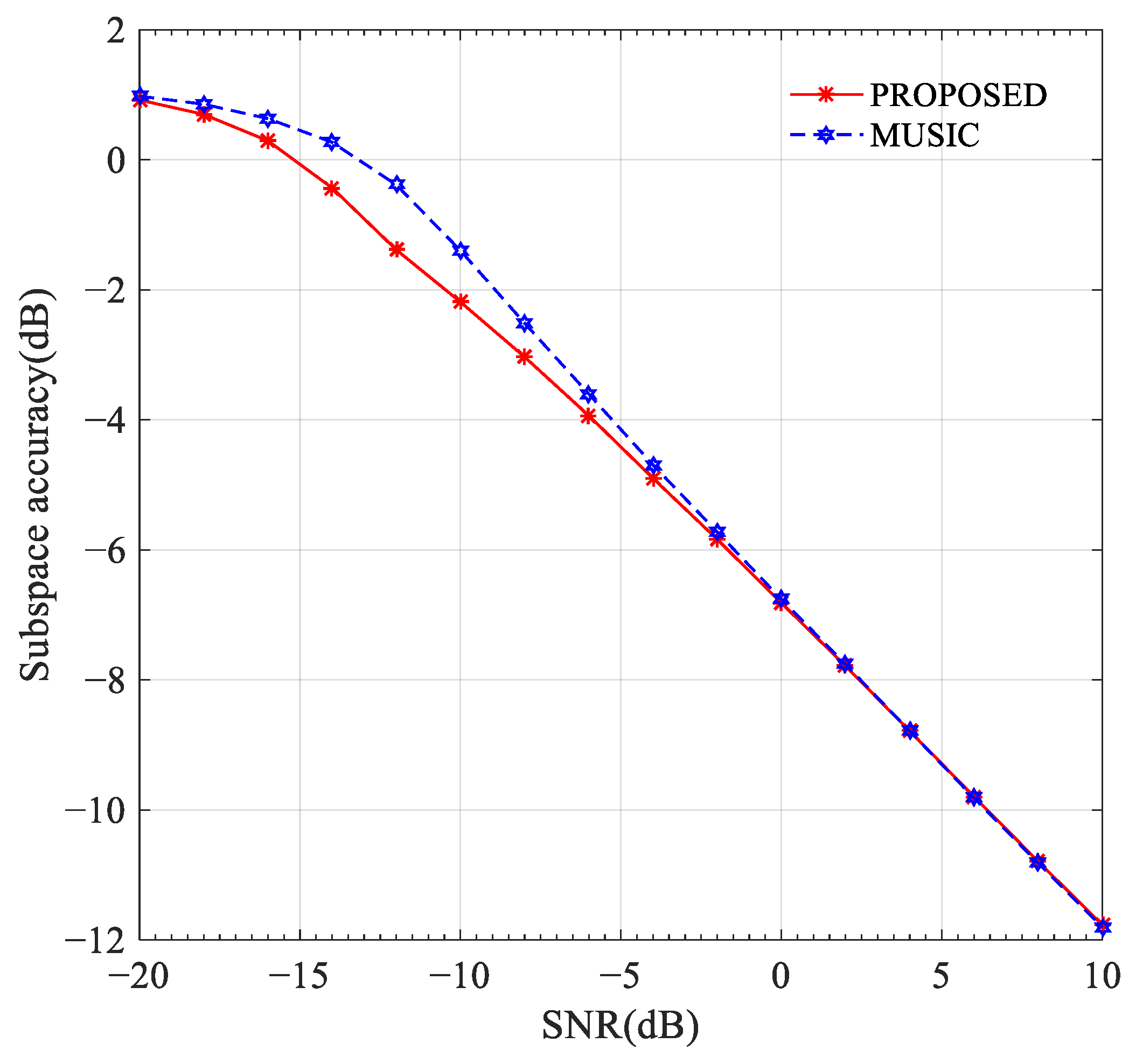
Figure 1. Accuracy of signal subspace versus SNR.
Remotesensing 14 04260 g001
Figure 2. Accuracy of signal subspace versus the number of snapshots.
Remotesensing 14 04260 g002
Figure 3. The number of iterations versus the input SNR.
Remotesensing 14 04260 g003
Figure 4. The number of iterations versus the number of snapshots.
Remotesensing 14 04260 g004
Figure 5. RMSE versus the input SNR.
Remotesensing 14 04260 g005
Figure 6. RMSE versus the number of snapshots.
Remotesensing 14 04260 g006
Figure 7. Spatial spectrum versus the input SNR.
Remotesensing 14 04260 g007
Figure 8. Spatial spectrum versus the number of snapshots.
Remotesensing 14 04260 g008
Figure 9. PSD versus elevation difference.
Remotesensing 14 04260 g009
Figure 10. PSD versus azimuth difference.
Remotesensing 14 04260 g010
Publisher’s Note: MDPI stays neutral with regard to jurisdictional claims in published maps and institutional affiliations.