
Sensitivity to Mass Changes of Lakes, Subsurface Hydrology and Glaciers of the Quantum Technology Gravity Gradients and Time Observations of Satellite MOCAST+

Abstract
:
1. Introduction
2. Method
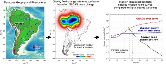
2.1. Method to Calculate the Gravity Signal, the Gravity Spectrum on the Sphere, and the Sensitivity to the Satellite Noise Spectrum
2.2. Definition of the Modelled Geophysical Gravity Signals-South America
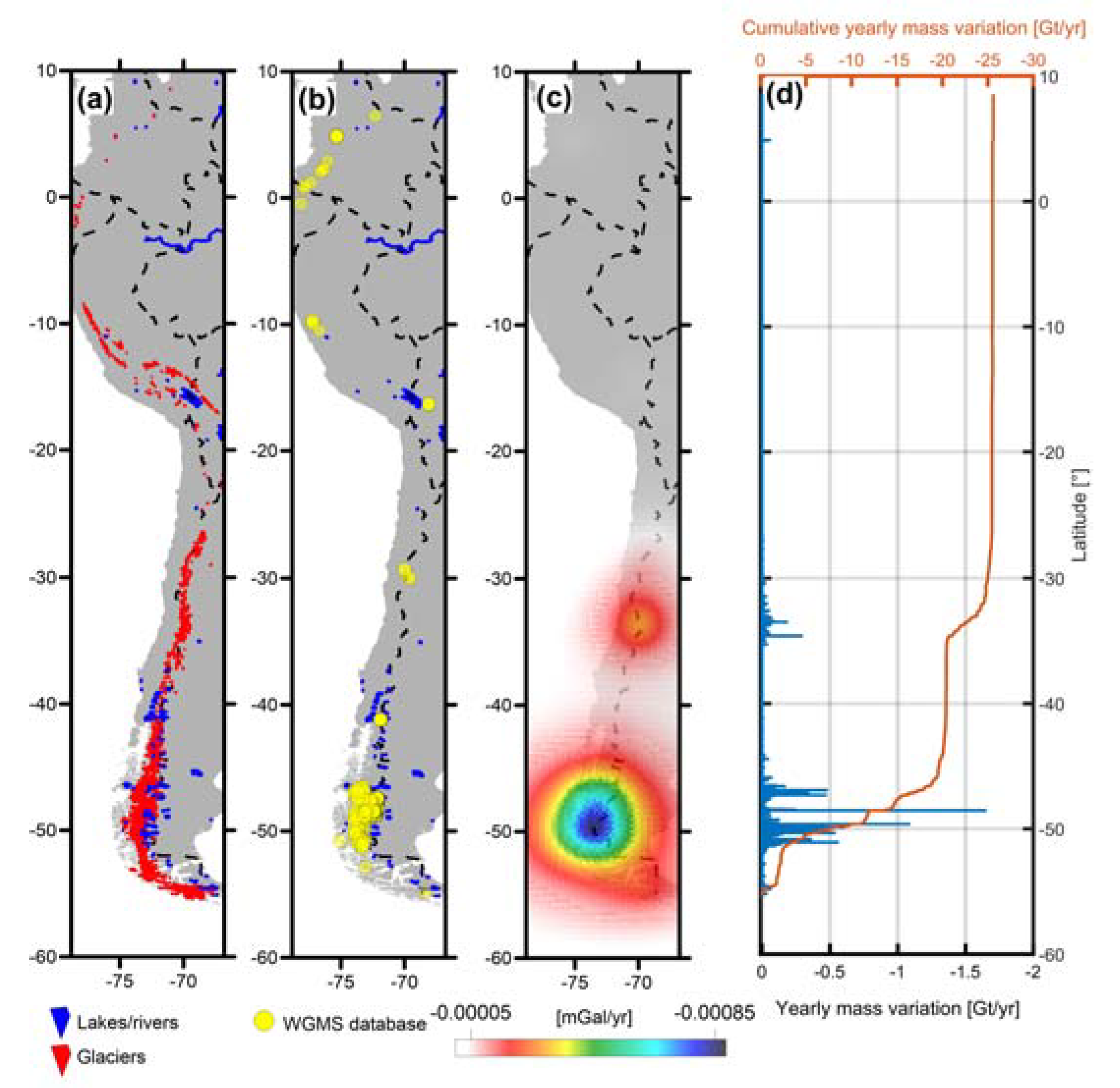
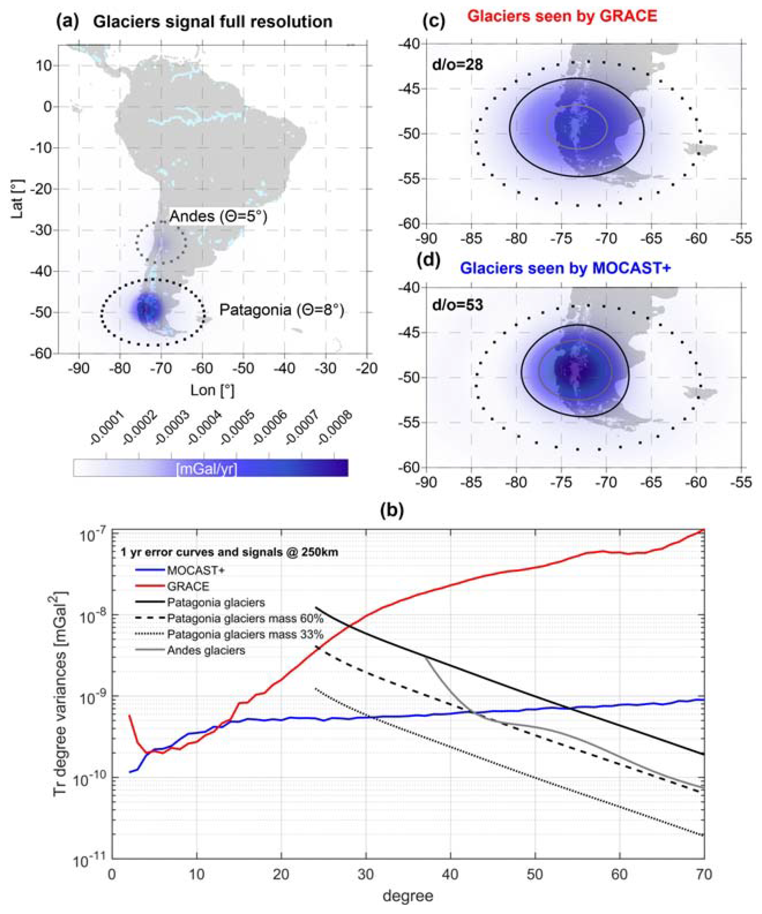
2.2.1. Glaciers
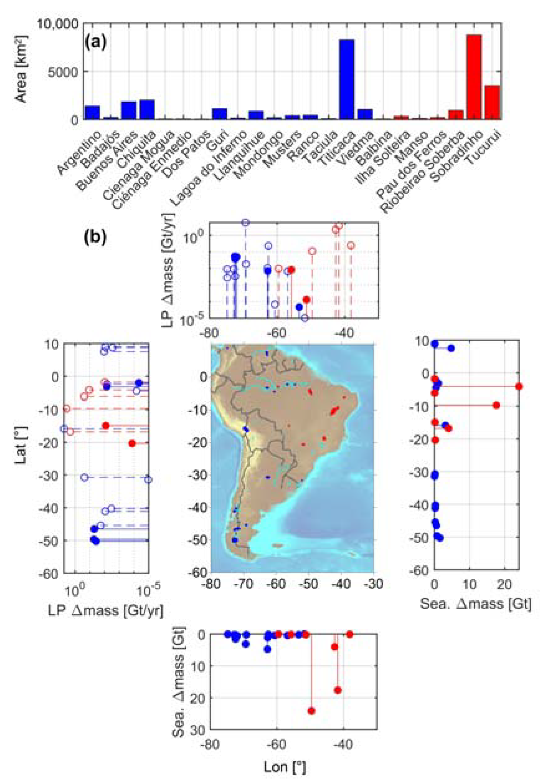
2.2.2. Lakes
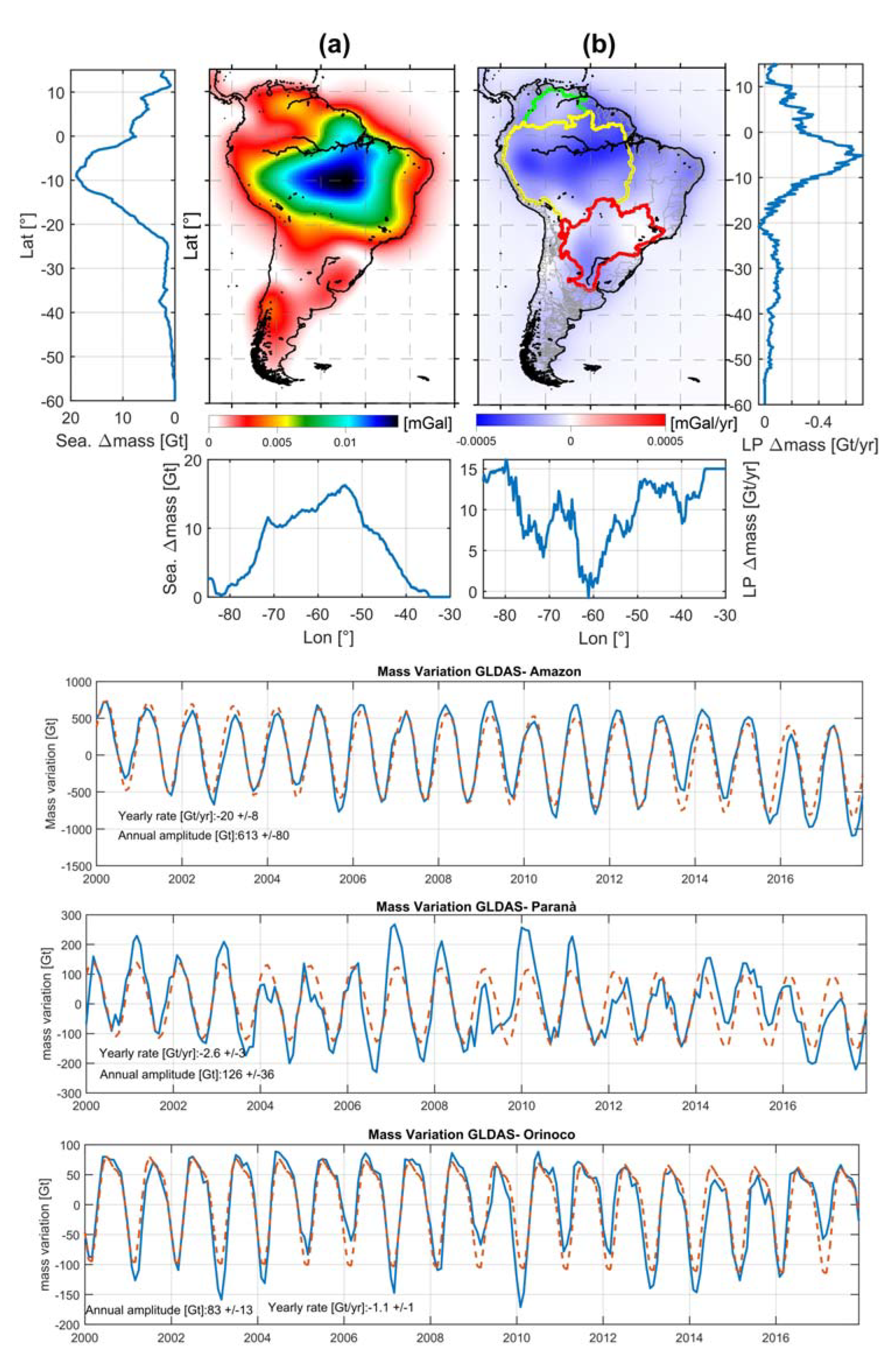
2.2.3. Soil Moisture Variations over SA
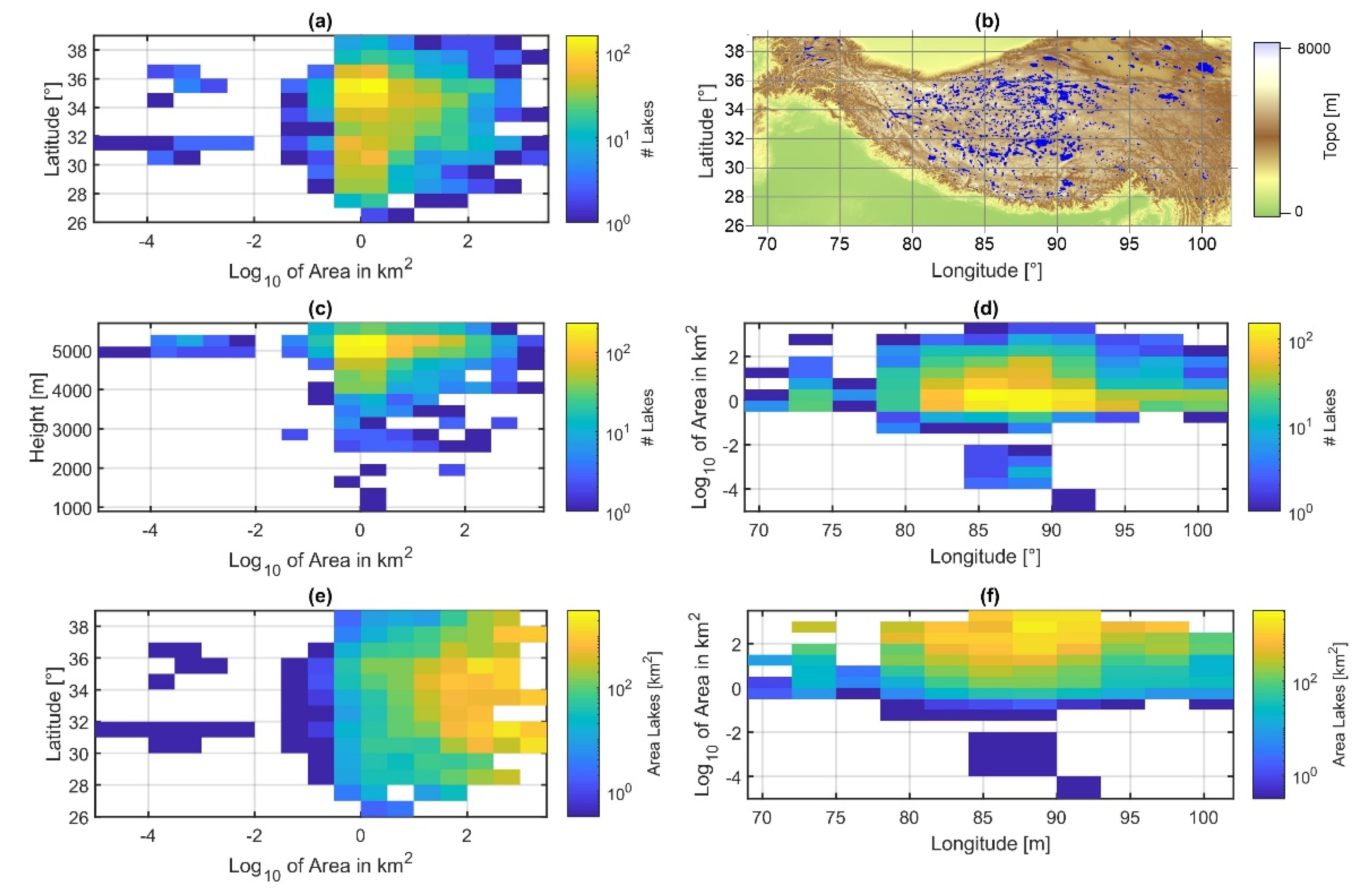
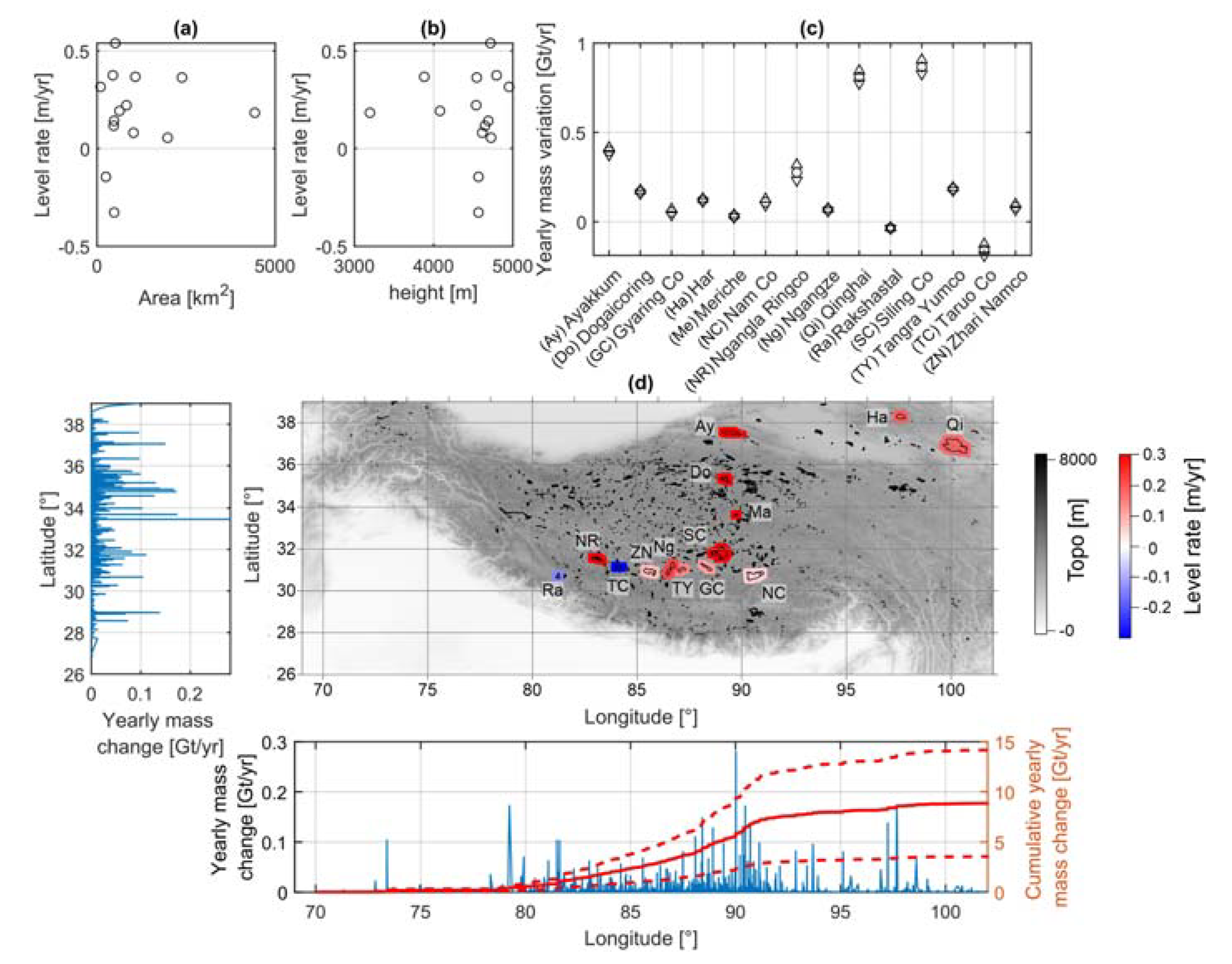
2.3. Lakes in the Tibetan Plateau
2.4. Summary of the Simulated Hydro-Glacio Phenomena and Gravity Signals
2.5. Definition of the Spectra of Geophysical Phenomena and the Error Curves of MOCAST+ and GRACE
3. Result
3.1. Sensitivity of MOCAST+ to Hydrology and Glaciers in the Andes
3.1.1. Sensitivity to South America Glaciers
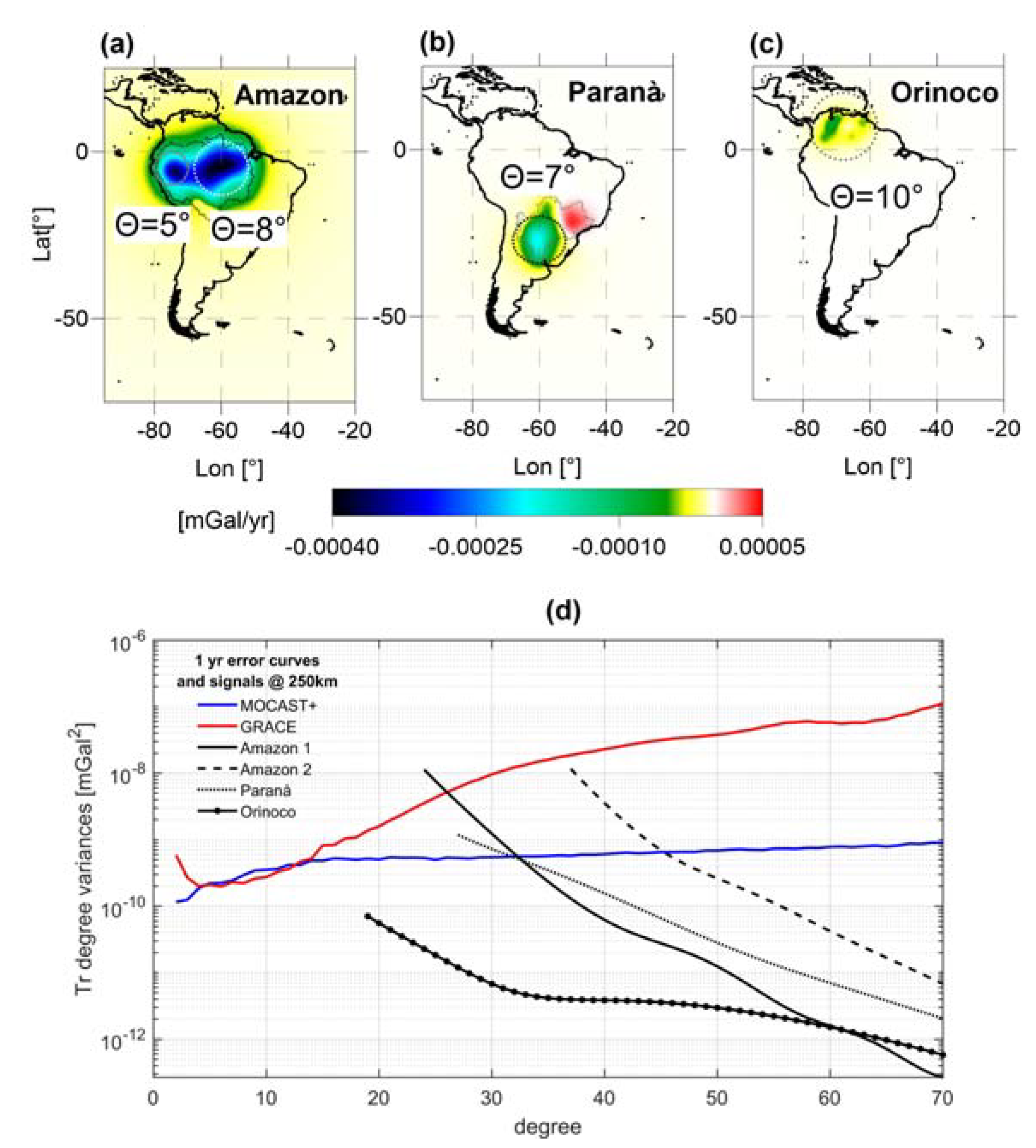
3.1.2. Sensitivity to Subsurface Hydrology in South America
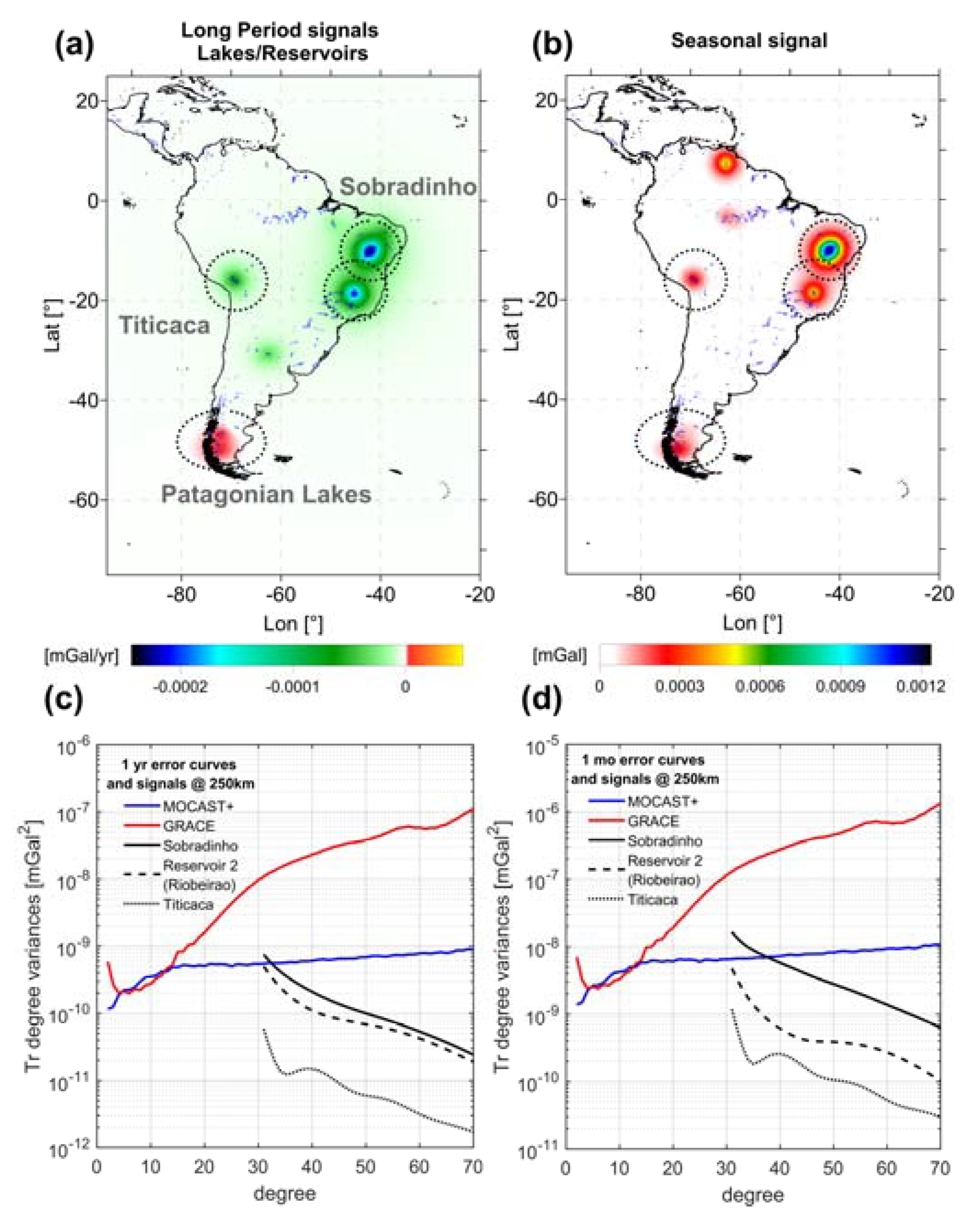
3.1.3. Sensitivity to Lakes/Reservoirs in South America
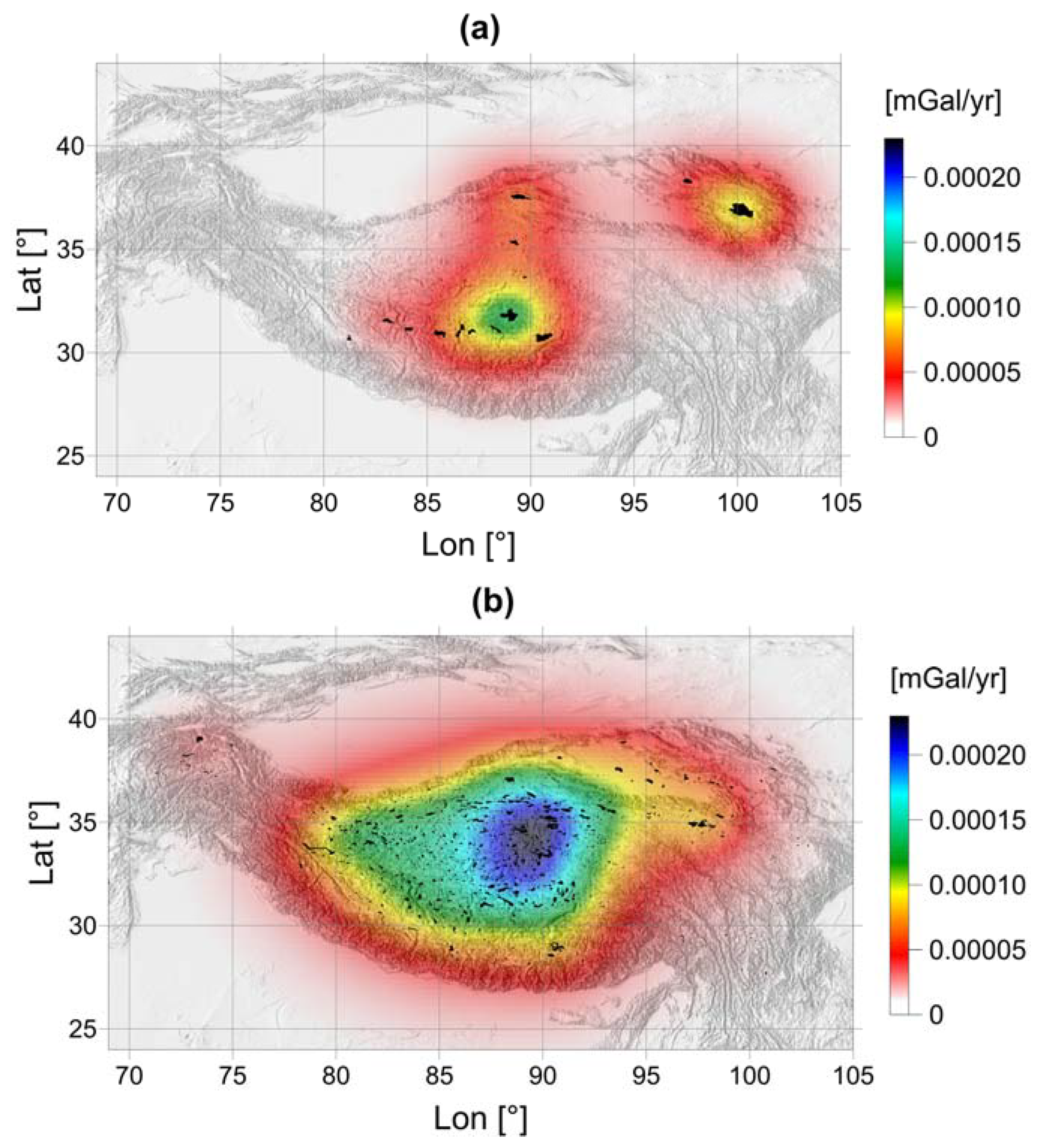
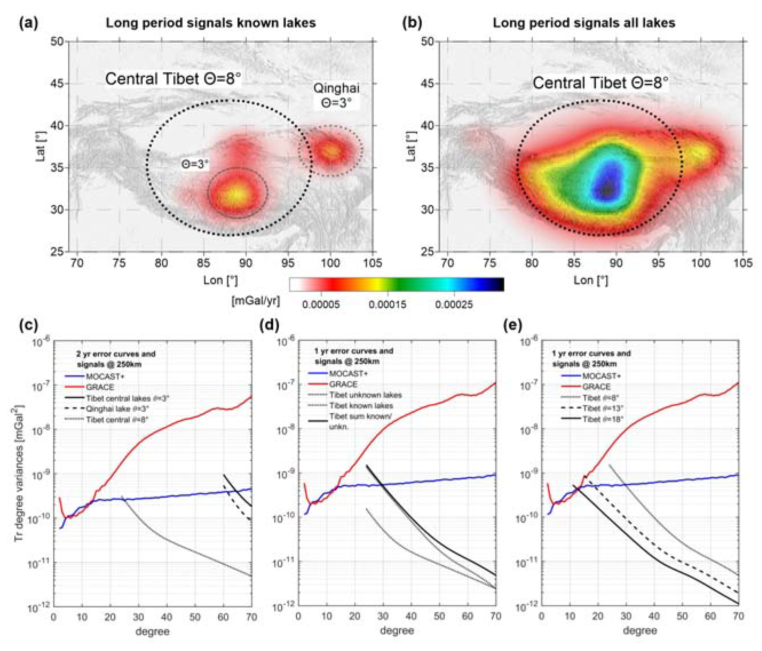
3.2. Sensitivity to Lake Hydrology in Tibet
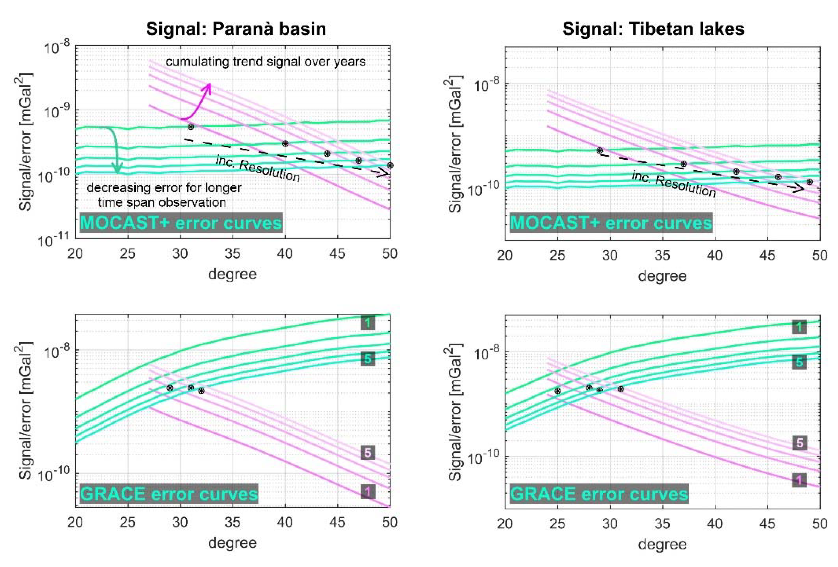
3.3. Trade-Off between Spatial Resolution and Time-Span of Observations
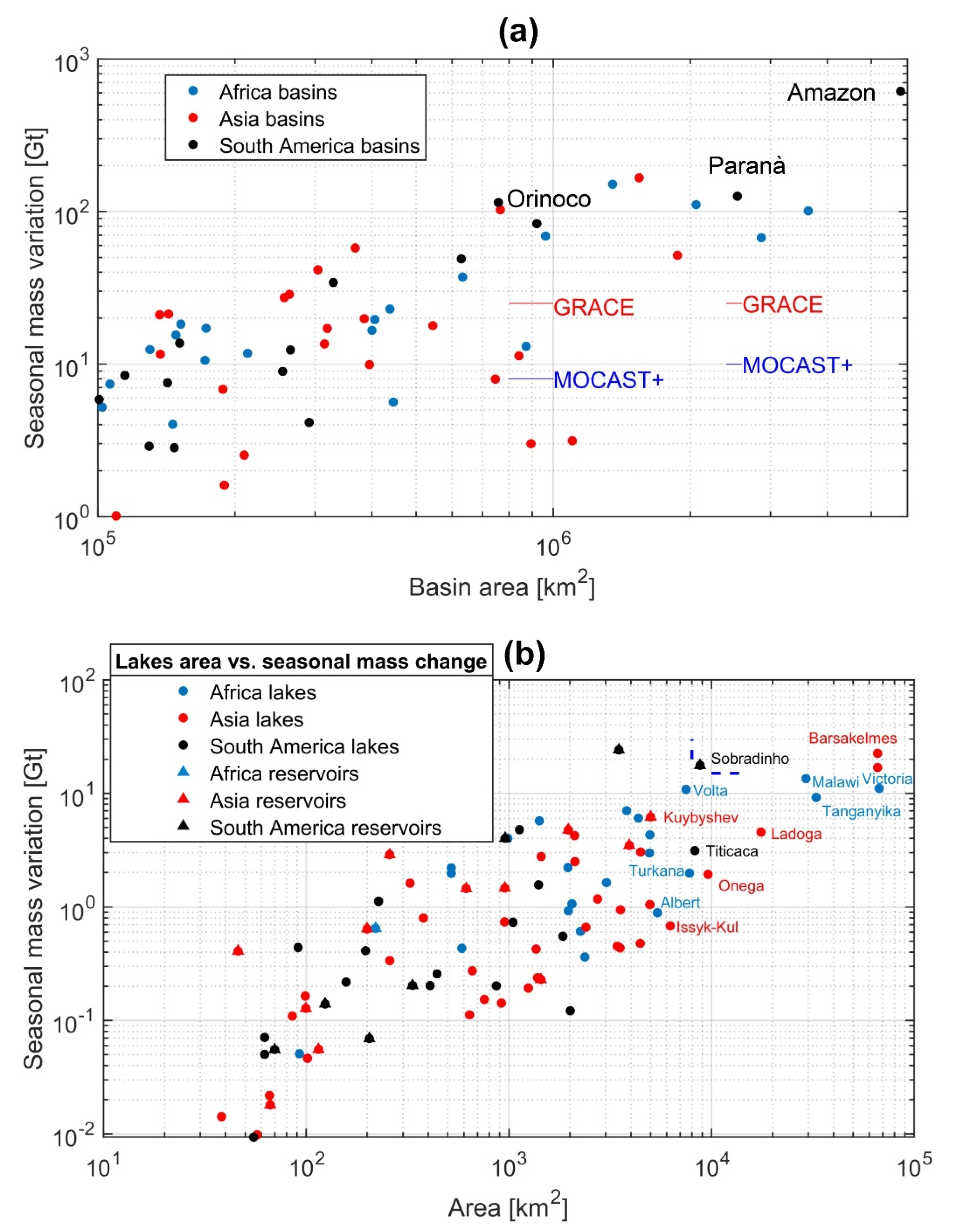
3.4. Setting the South American and Tibetan Lakes and Basins in a Global Context
4. Discussion
- -
- The ability to observe a larger number of phenomena (i.e., smaller glaciers, smaller basins);
- -
- An increase in the spatial resolution for the better characterization of a specific phenomenon;
- -
- An increase in the sensitivity to lower mass changes (i.e., sensitivity to lower deglaciation rates).
5. Conclusions
- The monitoring of seasonal components of reservoirs, lakes, and glaciers with areas > 8000 km2 and seasonal mass variations of 10 Gt: the estimate of the seasonal component allows for the retrieval of long-period trends with minor uncertainty;
- The sensitivity to deglaciation processes: in the case of Patagonian glaciers, the minimum rate observable with MOCAST+ amounts to 5 Gt/yr, an improvement compared to the GRACE observations, which detect a level of 10 Gt/yr;
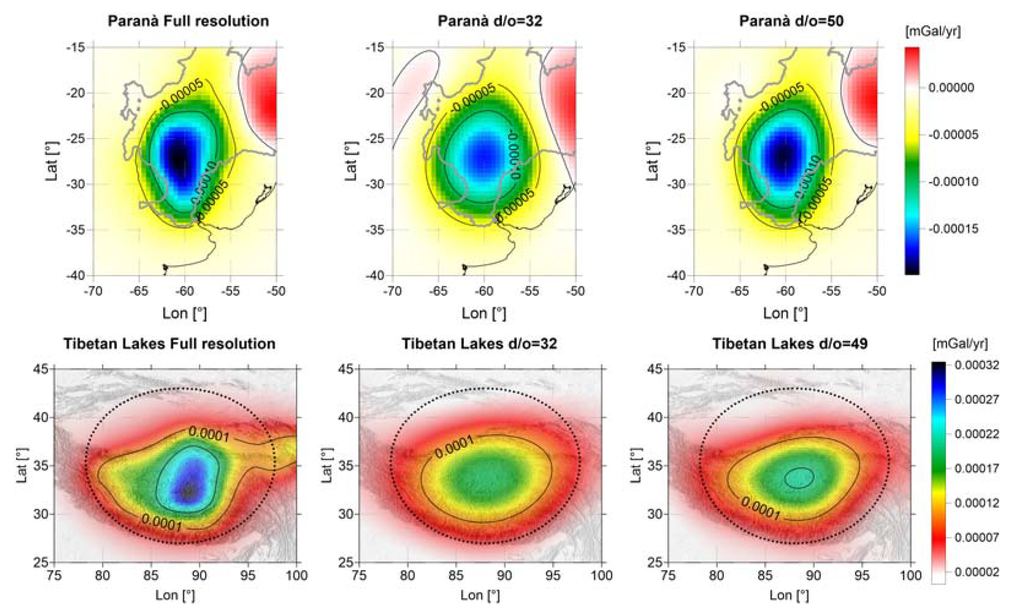
- The spatial resolution for the long-term monitoring of hydrologic basins and lakes: considering the example of the Tibetan lakes, which gain about 10 Gt/yr, MOCAST+ after 1 year resolves the variation that GRACE resolves after two years; after 5 years, MOCAST+ can retrieve the signal up to degree 50 in the spherical harmonic expansion, whereas GRACE resolves this signal only up to degree 32.
Author Contributions
Funding
Data Availability Statement
Acknowledgments
Conflicts of Interest
References
- Migliaccio, F.; Braitenberg, C.; Mottini, S.; Rosi, G.; Reguzzoni, M.; Sorrentino, F.; Tino, G.M.; Batsukh, K.; Koç, Ö.; Pastorutti, A.; et al. The MOCAST+ Study: Proposal of a Quantum Gravimetry Mission Integrating Atomic Clocks and Cold Atom Gradiometers. In Proceedings of the IAG Scientific Assembly 2021, Beijing, China, 28 June–2 July 2021; pp. 698–699. [Google Scholar]
- Rossi, L.; Reguzzoni, M.; Koç, Ö.; Migliaccio, F. Assessment of Gravity Field Recovery from a Quantum Satellite Mission with Atomic Clocks and Cold Atom Gradiometers. Quantum Sci. Technol. Spec. Issue Cold At. Space, 2022; under review. [Google Scholar]
- Migliaccio, F.; Reguzzoni, M.; Rosi, G.; Braitenberg, C.; Tino, G.M.; Sorrentino, F.; Mottini, S.; Rossi, L.; Koç, Ö.; Batsukh, K.; et al. The MOCAST+ Study on a Quantum Gradiometry Satellite Mission with Atomic Clocks. Surv. Geophys. 2022; under review. [Google Scholar]
- Migliaccio, F.; Reguzzoni, M.; Batsukh, K.; Tino, G.M.; Rosi, G.; Sorrentino, F.; Braitenberg, C.; Pivetta, T.; Barbolla, D.F.; Zoffoli, S. MOCASS: A Satellite Mission Concept Using Cold Atom Interferometry for Measuring the Earth Gravity Field. Surv. Geophys. 2019, 40, 1029–1053. [Google Scholar] [CrossRef]
- Pivetta, T.; Braitenberg, C.; Barbolla, D.F. Geophysical Challenges for Future Satellite Gravity Missions: Assessing the Impact of MOCASS Mission. Pure Appl. Geophys. 2021, 178, 2223–2240. [Google Scholar] [CrossRef]
- Reguzzoni, M.; Migliaccio, F.; Batsukh, K. Gravity Field Recovery and Error Analysis for the MOCASS Mission Proposal Based on Cold Atom Interferometry. Pure Appl. Geophys. 2021, 178, 2201–2222. [Google Scholar] [CrossRef]
- Kvas, A.; Behzadpour, S.; Ellmer, M.; Klinger, B.; Strasser, S.; Zehentner, N.; Mayer-Gürr, T. ITSG-Grace2018: Overview and Evaluation of a New GRACE-Only Gravity Field Time Series. J. Geophys. Res. Solid Earth 2019, 124, 9332–9344. [Google Scholar] [CrossRef]
- Massotti, L.; Siemes, C.; March, G.; Haagmans, R.; Silvestrin, P. Next Generation Gravity Mission Elements of the Mass Change and Geoscience International Constellation: From Orbit Selection to Instrument and Mission Design. Remote Sens. 2021, 13, 3935. [Google Scholar] [CrossRef]
- Flechtner, F.; Reigber, C.; Rummel, R.; Balmino, G. Satellite Gravimetry: A Review of Its Realization. Surv. Geophys. 2021, 42, 1029–1074. [Google Scholar] [CrossRef]
- Bender, P.L.; Wiese, D.N.; Nerem, R.S. A Possible Dual-GRACE Mission with 90 Degree and 63 Degree Inclination Orbits. In Proceedings of the 3rd International Symposium on Formation Flying, Missions and Technologies, Noordwijk, The Netherlands, 23–25 April 2008. [Google Scholar]
- Pastorutti, A.; Braitenberg, C.; Pivetta, T. Sensitivity to Geophysical Signals of the Quantum Technology Gravity Gradients and Time Observations on Satellite MOCAST+. Remote Sens. 2022; in preparation. [Google Scholar]
- Murböck, M. Virtual Constellations of Next Generation Gravity Missions; Technical University Munich: Munich, Germany, 2015. [Google Scholar]
- Purkhauser, A.F.; Siemes, C.; Pail, R. Consistent Quantification of the Impact of Key Mission Design Parameters on the Performance of Next-Generation Gravity Missions. Geophys. J. Int. 2020, 221, 1190–1210. [Google Scholar] [CrossRef]
- Heck, B.; Seitz, K. A Comparison of the Tesseroid, Prism and Point-Mass Approaches for Mass Reductions in Gravity Field Modelling. J. Geod. 2007, 81, 121–136. [Google Scholar] [CrossRef]
- Uieda, L.; Barbosa, V.C.F.; Braitenberg, C. Tesseroids: Forward-Modeling Gravitational Fields in Spherical Coordinates. Geophysics 2016, 81, F41–F48. [Google Scholar] [CrossRef]
- Pail, R.; Bingham, R.; Braitenberg, C.; Dobslaw, H.; Eicker, A.; Güntner, A.; Horwath, M.; Ivins, E.; Longuevergne, L.; Panet, I.; et al. Science and User Needs for Observing Global Mass Transport to Understand Global Change and to Benefit Society. Surv. Geophys. 2015, 36, 743–772. [Google Scholar] [CrossRef]
- Wieczorek, M.A.; Simons, F.J. Minimum-Variance Multitaper Spectral Estimation on the Sphere. J. Fourier Anal. Appl 2007, 13, 665–692. [Google Scholar] [CrossRef]
- Wieczorek, M.A.; Meschede, M. SHTools: Tools for Working with Spherical Harmonics. Geochem. Geophys. Geosyst. 2018, 19, 2574–2592. [Google Scholar] [CrossRef]
- Tapley, B.D.; Watkins, M.M.; Flechtner, F.; Reigber, C.; Bettadpur, S.; Rodell, M.; Sasgen, I.; Famiglietti, J.S.; Landerer, F.W.; Chambers, D.P.; et al. Contributions of GRACE to Understanding Climate Change. Nat. Clim. Chang. 2019, 9, 358–369. [Google Scholar] [CrossRef]
- Pfeffer, W.T.; Arendt, A.A.; Bliss, A.; Bolch, T.; Cogley, J.G.; Gardner, A.S.; Hagen, J.-O.; Hock, R.; Kaser, G.; Kienholz, C.; et al. The Randolph Glacier Inventory: A Globally Complete Inventory of Glaciers. J. Glaciol. 2014, 60, 537–552. [Google Scholar] [CrossRef]
- WGMS. Fluctuations of Glaciers Database; World Glacier Monitoring Service: Zurich, Switzerland, 2021. [Google Scholar]
- Wilson, R.; Glasser, N.F.; Reynolds, J.M.; Harrison, S.; Anacona, P.I.; Schaefer, M.; Shannon, S. Glacial Lakes of the Central and Patagonian Andes. Glob. Planet. Chang. 2018, 162, 275–291. [Google Scholar] [CrossRef]
- Lehner, B.; Döll, P. Development and Validation of a Global Database of Lakes, Reservoirs and Wetlands. J. Hydrol. 2004, 296, 1–22. [Google Scholar] [CrossRef]
- Schwatke, C.; Dettmering, D.; Bosch, W.; Seitz, F. DAHITI-an Innovative Approach for Estimating Water Level Time Series over Inland Waters Using Multi-Mission Satellite Altimetry. Hydrol. Earth Syst. Sci. 2015, 19, 4345–4364. [Google Scholar] [CrossRef]
- Rodell, M.; Houser, P.R.; Jambor, U.; Gottschalck, J.; Mitchell, K.; Meng, C.-J.; Arsenault, K.; Cosgrove, B.; Radakovich, J.; Bosilovich, M.; et al. The Global Land Data Assimilation System. Bull. Am. Meteorol. Soc. 2004, 85, 381–394. [Google Scholar] [CrossRef]
- Lehner, B.; Grill, G. Global River Hydrography and Network Routing: Baseline Data and New Approaches to Study the World’s Large River Systems. Hydrol. Process. 2013, 27, 2171–2186. [Google Scholar] [CrossRef]
- Zhang, G.; Ran, Y.; Wan, W.; Luo, W.; Chen, W.; Xu, F.; Li, X. 100 Years of Lake Evolution over the Qinghai–Tibet Plateau. Earth Syst. Sci. Data 2021, 13, 3951–3966. [Google Scholar] [CrossRef]
- Zhang, G.; Yao, T.; Shum, C.K.; Yi, S.; Yang, K.; Xie, H.; Feng, W.; Bolch, T.; Wang, L.; Behrangi, A.; et al. Lake Volume and Groundwater Storage Variations in Tibetan Plateau’s Endorheic Basin: Water Mass Balance in the TP. Geophys. Res. Lett. 2017, 44, 5550–5560. [Google Scholar] [CrossRef]
- Mayer-Gürr, T.; Behzadpur, S.; Ellmer, M.; Kvas, A.; Klinger, B.; Strasser, S.; Zehentner, N. ITSG-Grace2018-Monthly, Daily and Static Gravity Field Solutions from GRACE; GFZ Data Services: Potsdam, Germany, 2019. [Google Scholar] [CrossRef]
- Wouters, B.; Gardner, A.S.; Moholdt, G. Global Glacier Mass Loss During the GRACE Satellite Mission (2002–2016). Front. Earth Sci. 2019, 7, 96. [Google Scholar] [CrossRef]
- Drusch, M.; Donlon, C.; Scipal, K.; Schuettemeyer, D.; Veihelmann, B. Scientific Readiness Levels (SRL) Handbook; European Space Research and Technology Centre: Noordwijk, The Netherlands, 2015. [Google Scholar]
- Pivetta, T.; Braitenberg, C.; Pastorutti, A. Data Associated to “Sensitivity to Lakes, Subsurface Hydrology and Glaciers Mass Changes of the Quantum Technology Gravity Gradients and Time Observations on Satellite MOCAST+.” 2022. Available online: https://zenodo.org/record/6838878#.Yw1kHNNByUk (accessed on 15 July 2022). [CrossRef]


| Phenomenon | Localization | Area/Equivalent Circular Radius (r) or Equivalent Ellipse Semi-Axes (a, b) | Mass Change Seasonal Amplitude (Half-Peak2peak) | Gravity Change Seasonal @250 km Altitude. Full Spatial Resolution (Half-Peak2peak) | Mass Change Long-Term (Absolute Value) | Gravity Change Long-Term @250 km Altitude. Full Spatial Resolution | Spatial Scale = Radius of a Spherical Cap, Which Includes the Gravity Anomalies |
|---|---|---|---|---|---|---|---|
| Glaciers | Patagonia-Andes | 3 104 km2 a = 500 km b = 20 km | - | - | Single glacier: >1 Gt/yr Overall (clustering): 20–30 Gt/yt | 0.001 mGal/yr for Patagonia (clustering) | 8° including the whole Patagonia cluster |
| Natural Lakes | Whole South America | Titicaca 9 103 km2 R = 50 km | Single, 1–5 Gt | 0.0001 mGal | Generally <1 Gt/yr | <0.00001 mGal/yr for single lake (Titicaca) | 5–6° for single lake (i.e., Titicaca) |
| Reservoirs | Whole South America | Sobradinho 9 103 km2 r = 50 km | Single, can be >15 Gt | 0.001 mGal | <3 Gt/yr | Max 0.0002 mGal/yr for single reservoir | 5–6° For single reservoir (i.e., Sobradinho) |
| Natural Lakes | Tibet | Qinghai 4.5 103 km2 r = 35 km Whole Tibet 5 104 km2 r = 125 km | - | - | Single lake 1 Gt/yr (i.e., Qinghai); whole Tibet 11 Gt/yr | Single Lake 0.0001 mGal/yr; 0.0003 mGal/yr for clustering | 3–5° Single Lake 12–15° for whole Tibetan plateau |
| Sub-surface hydrology (Soil Moisture GLDAS) | Amazon basin | 6 106 km2 r = 1350 km | >600 Gt | >0.01 mGal | 20 Gt/yr | 0.0005 mGal/yr | 17° for whole basin. |
| Sub-surface hydrology (Soil Moisture GLDAS) | Paraná basin | 2.5 106 km2 r = 900 km | >100 Gt | 0.005 mGal | 2 Gt/yr | 0.0001 mGal/yr | 13° for whole basin |
| Sub-surface hydrology (Soil Moisture GLDAS) | Orinoco basin | 0.9 106 km2 r = 530 km | >80 Gt | 0.005 mGal | 1 Gt/yr | 0.0001 mGal/yr | 10° for whole basin |
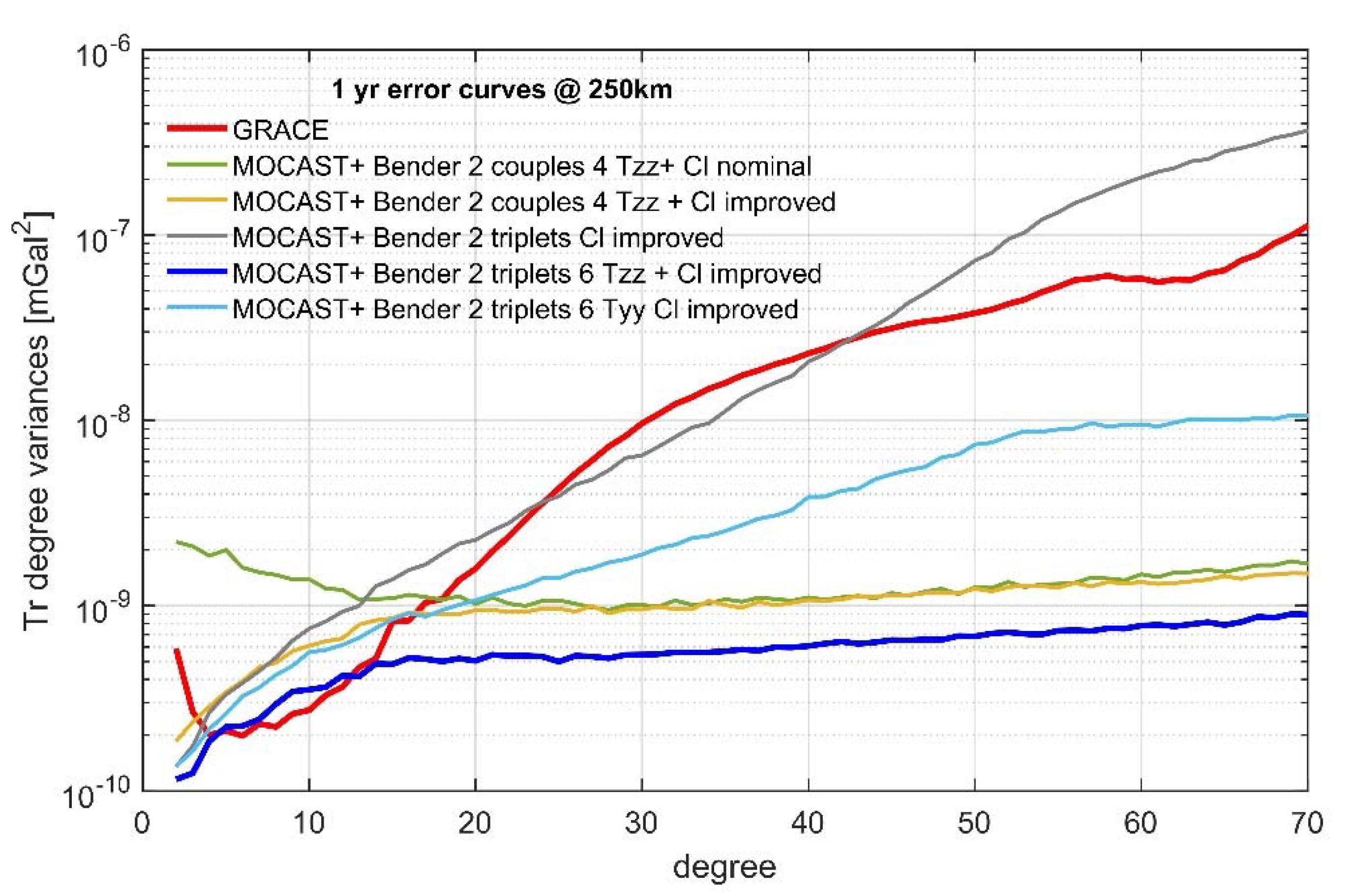
| Name Legend in Figure 8 | Configuration |
|---|---|
| MOCAST+ Bender 2 couples 4 Tzz+ Cl nominal | Bender configuration (2 couples, polar+inclined, 4 Tzz gradiometers) D = 100 km; 0.1 Hz clocks; optimal noise PSD for the gradiometers |
| MOCAST+ Bender 2 couples 4 Tzz + Cl improved | Bender configuration (2 couples, polar+inclined, 4 Tzz gradiometers), D = 1000 km, 1 Hz clocks, optimal noise PSD for the gradiometers |
| MOCAST+ Bender 2 triplets 6 Tzz + Cl improved | Bender configuration (2 triplets, polar+inclined, 6 Tzz gradiometers), D = 1000/2000 km, 1 Hz clocks, optimal noise PSD for the gradiometers |
| MOCAST+ Bender 2 triplets Cl improved | Bender configuration (2 triplets, polar+inclined), D = 1000/2000 km, 1 Hz clocks, clock-only solution |
| MOCAST+ Bender 2 triplets 6 Tyy Cl improved | Bender configuration (2 triplets, polar+inclined, 6 Tyy gradiometers), D = 1000/2000 km, 1 Hz clocks |
| Phenomenon | Mass Variation/Gravity Signal | GRACE | MOCAST+ (Best Configuration) |
|---|---|---|---|
| Glaciers’ long-term variations in Patagonia | Patagonia cluster: 20–25 Gt/yr; Area 30,000 km2; Cap area: 8°; Signal spectra 1yr: d/o 25 @ 250 km → Tr2 = 10−8 mGal2 d/o 45 @ 250 km → Tr2 = 2 × 10⁻⁹ mGal2 | -Detectable after 1yr. Max d/o 32 (λ/2 = 625 km). -Minimum rate observable (about 10 × 12 Gt/yr) | -Detectable after 1yr. Max d/o 53 (λ/2 = 380 km). -Minimum rate observable (about 5–8 Gt/yr) |
| Natural Lakes of South America: long-term trends | Lake Titicaca: 0.5–1 Gt/yr; Lake area 9000 km2; Cap area = 6° Signal spectra 1yr: d/o 32 @ 250 km → Tr2 = 7 × 10⁻¹¹ mGal2 d/o 45 @ 250 km → Tr2 = 1 × 10⁻¹¹ mGal2 | Lake Titicaca: not detectable even after 5 years | Lake Titicaca trend: detectable after more than 5 yr |
| Reservoirs of South America: long-term trends | Sobradinho: 2–3 Gt/yr; Reservoir area 9000 km2; Cap area= 6° Signal spectra 1yr: d/o 32 @ 250 km → Tr2 = 9 × 10⁻⁹ mGal2 d/o 45 @ 250 km → Tr2 = 1 × 10⁻¹⁰ mGal2 | Detectable after 5 years | Detectable after 2 years. |
| Natural Lakes in Tibet: long-term trends | Whole Tibet: 10–12 Gt/yr; Lakes area 50,000 km2; Cap area = 8° Signal spectra 1yr: d/o 25 @ 250 km → Tr2 = 0.5 × 10⁻⁹ mGal2 d/o 45 @ 250 km → Tr2 = 5 × 10⁻¹¹ mGal2 | Cumulative effect detectable after 2 years. Max d/o 26 (λ/2 = 770 km). | -Detectable after 1 year. Max d/o 28 (λ/2 = 715 km). -In 2 years increase in resolution with respect to GRACE. Max d/o: 34 (λ/2 = 590 km). |
| Amazon sub-surface hydrology (Soil Moisture GLDAS): Long-period trends | Amazon 1: 15 Gt/yr; Basin area 6 106 km2; Cap area = 8° Signal spectra 1yr: d/o 25 @ 250 km → Tr2 = 1 × 10⁻⁸ mGal2 d/o 45 @ 250 km → Tr2 = 5 × 10⁻¹¹ mGal2 | Detectable after 1 year. Max d/o 28. | Detectable after 1 year with higher resolution. Max d/o 32 (λ/2 = 625 km). |
| Paraná sub-surface hydrology (Soil Moisture GLDAS): Long-period trends | Paraná: 2–3 Gt/yr; Basin area 2.5 106 km2; cap area: 7° Signal spectra 1yr: d/o 28 @ 250 km → Tr2 = 1 × 10⁻⁹ mGal2 d/o 45 @ 250 km → Tr2 = 1 × 10⁻¹⁰ mGal2 | Detectable after 2 years | Detectable after 1 year. On the noise level. |
| Orinoco sub-surface hydrology (Soil Moisture GLDAS): Long-period trends | Orinoco whole basin: <1 Gt/yr; Basin area 0.9 106 km2; cap area: 10° Signal spectra 1yr: d/o 20 @ 250 km → Tr2 = 7 × 10⁻¹¹ mGal2 d/o 45 @ 250 km → Tr2 = 3 × 10⁻¹² mGal2 | Not detectable | Not detectable |
| Sub-surface hydrology (Amazon, Paraná, Orinoco): seasonal signals | Orinoco: 80 Gt; Basin area 0.9 106 km2; Cap area: 7° Signal spectra 1 month: d/o 28 @ 250 km → Tr2 = 1 × 10⁻⁶ mGal2 d/o 45 @ 250 km → Tr2 = 5 × 10⁻⁷ mGal2 | Detectable. Max d/o 35 (λ/2 = 570 km). | -Improvement in spatial resolution of monthly solutions. Max d/o 50 (λ/2 = 400 km). -Higher Sensitivity to smaller seasonal mass changes in basins. For a basin such as Orinoco 10 times smaller mass variations can be detected. |
| Lakes/Reservoirs in South America: seasonal signals | Sobradinho: 20 Gt/yr; Reservoir area 9000 km2; Cap area: 6° Signal spectra 1 month: d/o 32 @ 250 km → Tr2 = 7 × 10⁻¹¹ mGal2 d/o 45 @ 250 km → Tr2 = 1 × 10⁻¹¹ mGal2 | Hardly detectable | Sobradinho reservoir seasonal component detectable |
Publisher’s Note: MDPI stays neutral with regard to jurisdictional claims in published maps and institutional affiliations. |
© 2022 by the authors. Licensee MDPI, Basel, Switzerland. This article is an open access article distributed under the terms and conditions of the Creative Commons Attribution (CC BY) license (https://creativecommons.org/licenses/by/4.0/).
Share and Cite
Pivetta, T.; Braitenberg, C.; Pastorutti, A. Sensitivity to Mass Changes of Lakes, Subsurface Hydrology and Glaciers of the Quantum Technology Gravity Gradients and Time Observations of Satellite MOCAST+. Remote Sens. 2022, 14, 4278. https://doi.org/10.3390/rs14174278
Pivetta T, Braitenberg C, Pastorutti A. Sensitivity to Mass Changes of Lakes, Subsurface Hydrology and Glaciers of the Quantum Technology Gravity Gradients and Time Observations of Satellite MOCAST+. Remote Sensing. 2022; 14(17):4278. https://doi.org/10.3390/rs14174278
Chicago/Turabian StylePivetta, Tommaso, Carla Braitenberg, and Alberto Pastorutti. 2022. "Sensitivity to Mass Changes of Lakes, Subsurface Hydrology and Glaciers of the Quantum Technology Gravity Gradients and Time Observations of Satellite MOCAST+" Remote Sensing 14, no. 17: 4278. https://doi.org/10.3390/rs14174278