Abstract
Remotely sensed morphological traits have been used to assess functional diversity of forests. This approach is potentially spatial-scale-independent. Lidar data collected from the ground or by drone at a high point density provide an opportunity to consider multiple ecologically meaningful traits at fine-scale ecological units such as individual trees. However, high-spatial-resolution and multi-trait datasets used to calculate functional diversity can produce large volumes of data that can be computationally resource demanding. Functional diversity can be derived through a trait probability density (TPD) approach. Computing TPD in a high-dimensional trait space is computationally intensive. Reductions of the number of dimensions through trait selection and principal component analysis (PCA) may reduce the computational load. Trait selection can facilitate identification of ecologically meaningful traits and reduce inter-trait correlation. This study investigates whether kernel density estimator (KDE) or one-class support vector machine (SVM) may be computationally more efficient in calculating TPD. Four traits were selected for input into the TPD: canopy height, effective number of layers, plant to ground ratio, and box dimensions. When simulating a high-dimensional trait space, we found that TPD derived from KDE was more efficient than using SVM when the number of input traits was high. For five or more traits, applying dimension reduction techniques (e.g., PCA) are recommended. Furthermore, the kernel size for TPD needs to be appropriate for the ecological target unit and should be appropriate for the number of traits. The kernel size determines the required number of data points within the trait space. Therefore, 3–5 traits require a kernel size of at least . This study contributes to improving the quality of TPD calculations based on traits derived from remote sensing data. We provide a set of recommendations based on our findings. This has the potential to improve reliability in identifying biodiversity hotspots.
1. Introduction
Functional diversity of forests is essential for preserving the stability of terrestrial biodiversity. However, biodiversity is increasingly being threatened by climate change caused by large-scale, manmade changes to the biosphere [1,2,3]. Therefore, there is a need for regular monitoring of forest functional diversity, to effectively preserve and protect it. For this purpose, the Group of Earth Observation Biodiversity Observation Network (GEO BON), in collaboration with the broader biodiversity research community, developed a list of essential biodiversity variables (EBVs). The aim is to bridge the gap between ecological in situ observations and remotely sensed equivalents. EBVs represent an open framework of variables that are scalable, temporally sensitive, and ecologically meaningful [4,5]. Improving the understanding between EBV ecosystem structure and ecosystem functional diversity may help in achieving global biodiversity targets [6].
One of the major descriptors of ecosystem functions in terrestrial habitats is vegetation structure [7]. Vegetation structure in forests is quantified by measuring three-dimensional (3D) morphological traits such as tree height, canopy cover, and structural complexity [6]. These morphological traits have a mechanistic relationship to ecosystem properties (e.g., leaf area index, biomass, and carbon storage), indicating the status of ecosystem functions and services [6,8]. Structural EBVs aim to assess vertical and horizontal structural variability of vegetated habitats [4]. Several studies have suggested that while species richness is linked to ecosystem services, other diversity measurements, such as functional and structural diversity, are better predictors of key ecosystem functions and can capture changes in ecosystem functions that species richness does not reflect [9,10]. Information on species diversity and richness can be difficult to acquire, as all species need to be first located and then correctly identified, which is often a challenging task in forest environments [9,11,12]. Calders et al. [8], Schweiger et al. [12] showed that functional diversity measurements helped improve quantitative monitoring of changes in ecosystem functions. The habitat heterogeneity hypothesis, which predicts that species biodiversity increases with a greater habitat heterogeneity, does not necessarily apply to all species groups. Heidrich et al. [13] found that horizontal and vertical forest structure measures are, in most cases, good descriptors of habitat heterogeneity. However, a single universal mechanism determining a clear pattern and a unique relationship between habitat heterogeneity and biodiversity is still missing.
Recent studies have highlighted the need for high-spatial-resolution data capable of capturing individual plants [8,14]. Such fine detail enables new applications, for instance, delineating foliage of individual plants and detecting intraspecies trait variations [15,16,17], which subsequently improves the prediction of ecosystem properties [17]. Moreover, detailed spatial information about the habitat helps with modelling species distribution at local to regional scales [18] and improves our understanding of animal interactions with their habitats [19]. Other applications benefiting from high-spatial-resolution observations are mapping of fire fuel load and smaller ecosystem units such as canopy elements [20,21,22,23] or detection of habitat disturbances through size estimation of woody species populations that are more resilient to environmental fluctuations [24]. Therefore, quantifying morphological traits of individual plants can improve functional biodiversity mapping of local biotopes and regional ecosystems.
Several studies have demonstrated the capability of remote sensing techniques for measuring morphological traits across landscapes and natural ecosystems [6,25,26]. In particular, active light detection and ranging (lidar) technology has been proven to be highly effective in capturing 3D forest structure [6,27]. Lidar is effective in modelling forest understorey [28]. Other methods for capturing 3D forest structure, such as photogrammetric structure from motion (SfM) techniques, were found to be less effective in capturing the full canopy profile than lidar because lidar can penetrate the canopy deeper [29,30]. Although a variety of platforms has been used, lidar collections of high-density point clouds (e.g., 100 /−2), detailing leaves of individual trees, are often performed with on-ground sensors, i.e., by terrestrial laser scanning (TLS) or mobile laser scanning (MLS). Typically, such collections are limited to local plots with time requirements of 3–6 days per 1 [31]. In contrast to TLS and MLS, airborne laser scanning (ALS) and satellite platforms can cover large areas from landscapes to continents, but their point cloud density is significantly lower. Maintaining a relatively high point density, unoccupied aerial systems (UAS, popularly known as drones) mounted laser scanners (hereafter referred to as ULS) have the potential to (i) capture detailed morphological traits across local landscape scales, and (ii) link and upscale in situ TLS observations to ALS or spaceborne lidar observations [32,33].
The main advantage of UAS remote sensing is its ability to collect data at a variety of spectral, spatial, and temporal scales, tailored to the application requirements. UASs are capable of collecting data from which similar information can be extracted compared to in situ field observations but over larger areas, advancing the understanding of ecosystem functions through remote sensing [8,34,35]. Compared to other remote sensing platforms (e.g., full-size aircraft and satellites), UAS can be deployed on demand, regularly, and more frequently (under overcast conditions), allowing ecologists to observe phenomena, such as forest growth dynamics, in space and through time [8,36].
Schneider et al. [26] created a new framework for mapping functional diversity of forests with six remotely sensed morphological and physiological traits derived from airborne lidar and imaging spectroscopy data.These traits were combined in a multidimensional trait space, quantifying the hypervolume that samples/pixels occupy as a measure of functional diversity. This novel approach can be applied to map functional diversity across a range of scales, from an individual tree to landscapes [37,38]. It was later refined by adopting trait probability density (TPD) [37], developed as a measure of functional diversity by Carmona et al. [39]. TPD applies a kernel density estimation (KDE) that is more robust towards potential outliers in functional traits, but it requires input traits that are linked to specific ecological processes to be ecologically meaningful. A key question for any algorithm that is applied to fine-scale data, for which it was not originally designed for, is if it is capable of exploiting the full potential of these in situ data [8].
KDE is limited by the number of traits (dimensions) it can be applied to, with the recommended number of traits being 3–5 [40,41]. Selecting the appropriate traits requires careful consideration, as functional diversity indices derived from the trait hypervolume are sensitive to the number and type of traits [42]. Recent ecology studies have shown that only a small number of plant traits are sufficient to describe ecosystem functions [7,17]. High-point-density lidar can measure a large number of traits and, therefore, traits explaining the largest variance in the data and capturing key elements of 3D forest structure [6] must be selected first. However, certain applications require more plant traits (e.g., capturing intraspecies variations and gaining new functional information), in which case KDE might not be suitable. Reducing the number of dimensions through techniques such as the principal component analysis (PCA) or alternatives to KDE such as one-class support vector machine (SVM) might be more suitable when dealing with higher-dimensional hypervolumes [43,44]. These approaches have not been compared in remote sensing studies of functional diversity, and their practical implementations are unknown.
Schneider et al. [26] successfully demonstrated that ALS remote sensing can map the functional diversity of a European forest. Nevertheless, its scalability to higher-dimensional hypervolumes derived from fine-resolution morphological traits and high-density 3D point cloud data is yet to be tested. Our work aims to contribute to the assessment of functional diversity by providing new insights in assessing detailed ecologically meaningful traits at the spatial scale suitable for capturing individual trees. The original operational scientific contribution of our research is a workflow capable of assessing functional diversity of an Australian forest ecosystem in a high-dimensional space, at the local scale, suitable for long-term monitoring. In addition, we address questions about the applicability and limitations of the workflow. Specifically, we compare the variability in ULS-derived morphological traits to TLS-derived traits and evaluate the applicability of the TPD approach on high-dimensional ULS remote sensing data.
2. Methods
2.1. Study Site and Data Collection
The experimental ULS and TLS data were collected at the Terrestrial Ecosystem Research Network (TERN) supersite in Tumbarumba, located in the Bago State Forest in New South Wales, Australia (latitude: 35.6566°S, longitude: 48.1517°E, elevation: 1260 AMS), between 17 and 19 September 2019. The Tumbarumba site was selected for its past and perspective future contributions to the calibration and validation of satellite-derived Earth observation products. With an annual average rainfall of 1417 and a mean temperature of 9.8 [45], the site’s climate is considered as temperate. The soil type is classified as redoxic hydrosol and the vegetation type is an open wet sclerophyll Eucalyptus forest with two dominant tree species, mountain gum (Eucalyptus dalrympleana) and alpine ash (Eucalyptus delegatensis), gaining a maximum canopy height of 47 [45]. Figure 1 shows a canopy height model of the study site, which provides an indication of the distribution of tall trees. The study area is approximately large. After the data collection was completed, the study site was impacted by a natural bushfire event in the summer of 2019/2020.
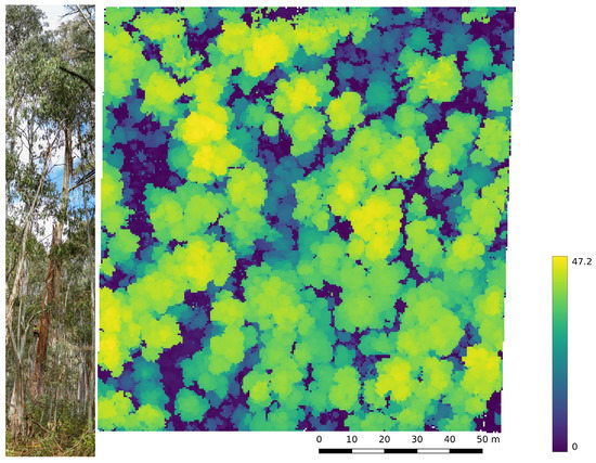
Figure 1.
Photo of the vegetation type on the left and canopy height map with 0.5m grid cell resolution of Tumbarumba on the right.
2.1.1. Terrestrial Laser Scanning
TLS data were collected with a Leica P30 ScanStation at a scan rate of 1 −1 and a maximum range of 270 [46]. The instrument has a survey-grade dual-axis tilt compensation and its laser point spacing was set to 3.1 at 10 . Additionally, it can capture RGB and high-dynamic-range (HDR) digital images of scanned objects. At the Tumbarumba study site, three plots of were established, and a scan was performed at every 10 , resulting in 16 scans per plot [31]. In every plot, four Leica black and white targets were distributed in addition to 12 styrofoam spheres used for co-registration of the scans. This sampling pattern was based on the sampling pattern for dense vegetation recommended by Wilkes et al. [31]. Three ground control points (GCP) were placed in each plot for georeferencing purposes. The coordinates for the GCPs were recorded with a dual-frequency real-time kinematic (RTK) global navigation satellite system (GNSS) receiver.
2.1.2. UAS Laser Scanning
A DJI Matrice 600 UAS airframe equipped with a Velodyne VLP-16 Puck lidar scanner was employed for the UAS data collection [47,48,49,50]. The UAS lidar acquired laser returns at a height of 10 –15 above the top of the canopy or around 60 above ground (depending on the local topography) at a flying speed of 3 −1, using a “lawnmower” (overlapping parallel flight lines) pattern with a side overlap of 50%. The lidar sensor was set to a scanning frequency of 66.667 −1 with an across-track field of view of 80. The Velodyne scanner has an along-track field of view of 30 with 16 parallel scan layers separated by 2. This configuration allows laser beams to penetrate the canopy in nadir and oblique angles with a resulting point density of 1491.33 −2. The flight speed was matched to the scan frequency with the aim of achieving an even point density along and across the track.
2.2. Lidar Data Processing
A standardisation preprocessing workflow was applied before extraction of morphological traits of interest. Since TLS and ALS datasets have fundamental differences in point distribution throughout the canopy [51], caused by different sensor positioning, we attempted to reduce these differences through voxelisation. The TLS data were spatially co-registered and georeferenced using the collected GCPs, while the ULS point cloud was directly georeferenced based on onboard GNSS and IMU observations. ULS GNSS data were post-processed against GNSS base-station data acquired at 10 frequency. An in-house Python script for direct georeferencing was applied to produce ULS LAS files from raw scans and post-processed GNSS and IMU data. A graphical overview outlining the workflow for TLS and ULS data processing is presented in Figure 2.
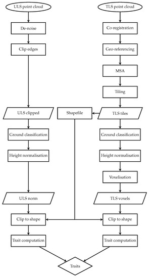
Figure 2.
Flowchart showing processing workflows designed forTLS and ULS data interpretations into morphological functional traits.
The TLS data were processed per-plot with the Leica Cyclone Register 360 software [52]. Scans of each plot were spatially co-registered and georeferenced by marking the GCPs as targets in the point clouds and assigning them with the reference coordinates collected in the field through an RTK GNSS survey. The co-registration in Register 360 was, however, inaccurate and showed signs of a point cloud “ghosting” (point clouds were not correctly aligned and branches appearing twice). Therefore, the TLS point clouds were imported into the RiSCAN PRO 2.10 software [53] followed by manual co-registration based on the Multi Station Adjustment Plugin (MSA). The MSA was applied to improve the accuracy of the co-registration, with an error . The MSA makes an optimisation of all scan positions, matching the point clouds from neighbouring scans.
The scans were merged and then tiled to be compatible with our airborne laser scanning workflow. Based on the scanner locations, a polygon shapefile including a 5 buffer was created to select the core area of the scans. The point clouds were ground-classified and height-normalised in the LASTools software [54]. A voxelisation of was applied to achieve a similar point spacing to the ULS point cloud at the top of the canopy.
Raw data acquired with the ULS payload Velodyne Puck were converted into the LAS file format with a custom-built script. Noise in ULS data was reduced by applying the noise filtering algorithm in LASTools and by manually removing outliers above known canopy height and below ground in the CloudCompare software [55]. To classify ground and to normalise the ULS point cloud, the same processing steps as for the TLS point clouds were applied in LASTools. To match the spatial extent, both point clouds were clipped based on the earlier-created plot polygon layer, thereby removing the points at cloud edges and avoiding edge artefacts. The final computation of morphological traits is discussed in the following section.
2.3. Morphological Traits
Selection of morphological traits from the literature applied the following criteria: (i) ecological meaningfulness, (ii) relation to at least one ecosystem function (e.g., primary productivity), (iii) relevance to functional diversity assessment, (iv) wide acceptance in the peer-reviewed literature, and (v) need for minimum prior knowledge about the studied vegetation. Additionally, traits needed to be scalable across operational scales, specifically from TLS to ALS, applicable to a wide range of lidar platforms, and capable of being a part of an area-based workflow producing raster maps. Seven traits that met the above-listed criteria were selected and are presented in Table 1.

Table 1.
Overview of traits and axis captured.
Our literature review revealed some variations in definitions of morphological forest variables. Therefore, the traits of interest, in the context of this study, are defined as follows: canopy height () describes the maximum vertical distance between the top of canopy and ground. It is a critical variable for quantifying forest biomass, carbon stocks, growth, and primary productivity, and it has been related to species richness [58,65]. Effective number of layers () is based on several measures of diversity and further advances the concept of the foliage height diversity () [59,66].
is described by the three variables , , and , defined as:
where is the proportion of points in the ith vertical layer of the sum of all points in a point cloud [59,60]. The thickness of the vertical layers was set to ( 1 ). computes the total number of layers in the point cloud that is equivalent to canopy height. Similar to , is based on the Shannon diversity index [60]. It was used in several studies and is positively related, for instance, to bird diversity [26,37,60,61,67,68,69]. is based on the Simpson diversity index; however, it does not utilise the natural logarithm of . This is advantageous for high-point-density clouds, as occlusions and small gaps in the vertical layer profile can lead to empty layers to which the logarithm cannot be applied. Therefore, uses the square of , which remedies this issue. Use of is more intuitive because, unlike , its high values indicate a high vertical structural variability [59].
The canopy ratio () is calculated as the percentage of canopy depth to canopy height and is defined as:
where is the relative height as percentiles of the vertical distribution of points at 25 and 98%, respectively.
Rugosity (R) is a measure of structural heterogeneity and a frequently used indicator of forest structural changes and habitat complexity [6,8,16,70]. It is defined as the standard deviation of canopy height [71,72].
Gap fraction () is based on Beer’s law regarding gap fraction theory [73]; it measures the vertical openness of the canopy and is, therefore, related to total forest biomass [74]. summarises the fraction of lidar points that reach a defined forest canopy layer and those that pass through the layer as:
where is the number of returns below a given height z, and is the total number of returns. is the number of returns below , with being the thickness of the layer set to 1 [62].
Leaf area density () was designed to provide information about the vegetation understorey and is based on .
with k being the extinction coefficient and set to 0.25, which is suitable for a canopy with an erectophile distribution of leaf inclination angles of eucalypts [75,76].
and are based on Beer’s law, which is used to estimate the leaf area index for large-footprint full-waveform lidar [77]. In this case, and are categorised as vertical traits along the x, y axis (see Table 1).
Plant–groundratio () is equal to the plant area index, as described in Schneider et al. [63], but applied solely to the first and the last lidar returns. As a simplified lidar proxy of leaf area index, it describes the ratio between the number of ground points and other points in the canopy point cloud.
Box dimensions () is a fractal analysis of the 3D shape of a point cloud designed to gain better insight into the shape of individual trees and the architectural cost–benefit ratio [64]. It is sensitive to the outer shape and internal structure of trees. describes how many voxels are required to enclose all elements of a 3D point cloud and how this number changes with the ratio of the size of the voxel. Seidel et al. [64] found a positive relationship between and growth performances of individual trees. We assume that can describe a similar relationship when applied with an area-based approach instead of on individual trees.
Extraction of the above-mentioned morphological variables from the ULS and TLS point clouds was performed in R [78] using the lidR package [79]. Each variable can be derived per point cloud (e.g., a whole study site or its plots) but also as a grid metric, where the trait is calculated per individual grid cell, and can be displayed as a 2D grid layer. The two-dimensional grid layers, capturing spatial variation, are suitable to assess the spatial variability of morphological variables within a site or its sub-plots.
2.4. Applicability across Spatial Scales
The above-described morphological traits are expected to resolve not only high-density TLS point clouds but also lower-point-density ULS and, ultimately, ALS data. To assess the impact of spatial scale and grid resolution on trait retrieval, we tested a range of grid cell sizes from 0.5 up to 5 . For reference, Table 2 provides an overview of the different lidar platforms and their suitability to deliver products with different grid cell sizes, ranging from typical TLS (around ) through ULS and ALS (above ), up to the spaceborne lidar GEDI (which stands for Global Ecosystem Dynamics Investigation program, and is the first spaceborne lidar designed to measure vegetation structure) (25 m ø) [25,80].

Table 2.
Overview of grid sizes for different lidar platforms. + indicate the suitability of the grid size for the platform.
2.5. Statistical Analysis
To assess the variance in morphological traits derived from TLS and ULS scans of the three study plots, statistical analyses were performed per trait at a given grid size between the three plots. All traits were scaled between 0 and 1, with a % cutoff at the top and bottom range to remove outliers [37]. Wilcoxon rank sum tests were applied to calculate correlation coefficients and derive linear, power-law, and logarithmic regressions. Variance among the plots was representative for the whole study site. For further analysis, the data of the three study plots were merged into a single dataset. In addition to the tests mentioned above, a PCA was performed to assess the variability between TLS and ULS-derived traits [37]. To simulate different spatial scales, these tests were performed at multiple grid sizes listed in Section 2.4, aiming to assess suitability of traits obtained from different lidar platforms. Selection of traits for the next analytical step was performed based on the obtained results.
2.6. Trait Probability Density
Trait probability density (TPD) is based on an n-dimensional hypervolume called trait space, using traits as the axes. TPD within the trait space was calculated by modelling the data through KDE and estimating the density along the n-dimensional sampling grid with 0.1 trait intervals (equivalent to 10 bins along each trait axis) [37,39]. For a trait space based on three traits, the sampling grid becomes a 3D object of voxels. Computational resources required to apply KDE to an n-dimensional hypervolume increase exponentially with the number of dimensions (traits) of the hypervolume. Therefore, applying KDE to large datasets of high dimensionality is computationally demanding [81]. It is, therefore, recommended to use this approach only for 3–5 traits [40,41]. Different techniques can be applied to reduce the number of traits. For example, traits can be selected based on (i) ecological meaningfulness (see Section 2.3), (ii) reduced reciprocal correlation and high PCA loading (see Section 2.5), and (iii) core trait functionality capturing at least the canopy height, cover, and structural complexity [6] (see Table 1). If trait selection reduces the number of traits insufficiently or the case requires use of more traits, methods such as dimensionality reduction (e.g., PCA) or alternative approaches such as SVM might be required [43,44]. The number of dimensions might be reduced through PCA, striking a balance between the number of PCA components retained and the percentage of variance-explained. Optionally, a machine learning approach such as an SVM classifier can group data into one or two classes. SVM replaces KDE in the trait space and assesses if points lie inside or outside the hypervolume along the sampling grid [81]. In comparison to KDE, the SVM cannot calculate the density of data as it only models the decision boundary between samples inside and outside the hypervolume. SVM could be more suitable for highly dimensional hypervolumes [44].
Independent of the method used, the TPD approach, originally proposed by Carmona et al. [39], Villéger et al. [43], uses three functional diversity indices to describe the shape of the hypervolume in trait space: functional richness (), functional evenness (), and functional divergence (). describes the volume of function space occupied by traits [37,43]. is based on the O index proposed by Bulla [82], describing the evenness in the distribution of occupied trait space [83]. is another measure for the distribution of TPD in the trait space. It indicates if the occupied trait space is distributed more towards the edges of the space or centred in the middle [83]. Before calculating these functional diversity indices, a threshold of >2 data points per cell in the sampling grid was applied to the density estimated by the KDE-based TPD to reduce the influence of outliers. Therefore, the indices were based on at least two estimated data points. No threshold was applied to SVM-based TPD because it does not provide a density estimate.
We applied KDE based on a Gaussian kernel with a bandwidth of 0.1 [37]. PCA components were selected to retain 90 % explanatory power; however, due to the trait selection (see Section 2.5), this often resulted in only 2–3 components being used. Our SVM classifier used a radial basis function kernel with set to 0.1 and at 0.9 to achieve results that were similar to KDE [44]. TPD was applied to the raster-based traits through a moving-window approach with a kernel size of . Based on the recommendation by Blonder et al. [84], the kernel size of elements was chosen to ensure a relationship. Furthermore, this kernel size was sufficient to capture larger canopy elements at a grid cell size of as our target ecological unit.
Computation of TPD was implemented in Python using the scikit-learn Density Estimation module [85]. The code was executed on a Windows server with an Intel Xeon E5-2637 v3 @ CPU and 256 GB RAM. A sensitivity analysis was performed on an artificial simulated dataset to assess the influence of number of dimensions and kernel size on the functional diversity output and computation requirements. All analyses were performed with multiple iterations (n = 10) and the mean and standard deviation are presented where relevant. The first dataset contained a varying number of dimensions, where each dimension comprised 80 data points, simulating a kernel. The second dataset had a fixed number of four dimensions, but varying number of data points per dimension. We measured the time that each of the three approaches needed to process these datasets. Next, we applied the three approaches with the moving-window, with a kernel size of pixels, to traits derived from a ULS point cloud of the whole Tumbarumba study site to assess their performance and outputs. The trait grid layers had dimensions of and consisted of four traits: , , , and (see Section 3.1). We limited the number of traits to four due to computer resource limitations for computation of the FD maps. While out-of-memory processing is possible, we assumed that typical end-users do not have the required high-performance computing infrastructure or the technical capabilities to implement it. Furthermore, an increase in the number of dimension results in an exponential increase in required memory, with 11 traits resulting in 2 TB of random access memory (RAM) requirements.
3. Results
3.1. Statistical Analysis
The data points from the three TLS plots were combined to capture the variation in traits across the study site. ULS and TLS traits have similar characteristics, as can be seen by comparing Figure 3a,b. These two figures only show a subset of the traits; the full plots can be seen in Figure A1 and Figure A2 in Appendix A.1.1. Appendix A contains the outputs for ULS and TLS traits, organised by grid size ( , 1 , and 5 ). The output of the correlation analysis can be found in Appendix A.1.2, Appendix A.2.2 and Appendix A.3.2, and Wilcoxon tests are presented in Appendix A.1.3, Appendix A.2.3 and Appendix A.3.3. The outputs of the linear regression analysis and PCA explained variation and loadings are in Appendix A.1.4, Appendix A.2.4 and Appendix A.3.4 and Appendix A.1.5, Appendix A.2.5 and Appendix A.3.5, respectively. The outputs of the logarithmic and power-law regression are not included because they did not contain any significant findings.
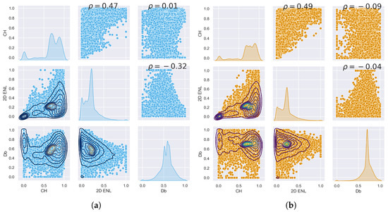
Figure 3.
Pair plot comparing , , and between each other for ULS (blue) and TLS (orange). (a) Selection of ULS traits. (b) Selection of TLS traits.
For area-based traits, had higher PCA loadings for components 1–3 for both TLS and ULS compared to and (see Figure A14, Figure A15, Figure A16, Figure A17, Figure A18 and Figure A19 in Appendix A.1.5). PCA loadings were generally higher compared to . showed the highest correlation and significant linear relationship between ULS and TLS of all variables across the different grid sizes. Another potential trait was , as it consistently had the highest PCA loading of all traits, which is consistent with other studies [37]; however, we limited the number of traits to four due to computational memory constraints.
3.2. Trait Probability Density
The three approaches for computing TPD are presented in two parts. First, we present a sensitivity analysis based on artificial datasets to assess the impact of the number of dimensions and number of data points on the TPD output and computation time. In the second part, we present a remote sensing example of applying the three methods to real-world data for the Tumbarumba study site.
Comparing the TPD outputs of KDE, KDE+PCA, and SVM in relation to the number of dimensions provides insight into how sensitive each approach is to a varying number of traits and how well they can be compared with each other.
TPD outputs for KDE, KDE+PCA, and SVM in relation to the number of dimensions are presented in Figure 4. These results show that TPD outputs for the SVM and KDE approaches can only be produced for up to five and six dimensions, respectively, due to memory constraints. The general trends of the TPD outputs are consistent in relation to the number of traits; however, some outliers exist. In Figure 4a, of SVM is significantly higher compared to of KDE, and it shows a clear decline with an increase in dimensions. of KDE decreases slightly with an increase in the number of dimensions, while PCA-based stays consistent and similar to KDE-based for three and four dimensions. All (Figure 4b are identical from all three methods and did not change with an increase in the number of dimensions. Figure 4c shows that values for KDE and PCA are identical and show an increase with an increase in the number of dimensions from three to four, but then drop to around 0 at five dimensions. for SVM is at 0.

Figure 4.
Chart comparing TPD outputs between KDE, KDE+PCA, and SVM in relation to the number of dimensions. (a) Functional richness. (b) Functional evenness. (c) Functional divergence.
Computation time is an important consideration when choosing an approach. Here, we compare the computation for calculating , , and between the three different approaches versus only applying KDE, KDE+PCA, and SVM without calculating the TPD outputs. The line represents the mean time of multiple iterations (n = 10) and the shaded area represents the standard deviation.
Comparing Figure 5a,b, strong differences in performance between the three approaches can be observed, indicating that the calculation of the TPD output itself has an impact on performance in terms of computation time and computer resources. As stated above, SVM only managed to calculate TPD outputs for five dimensions, due to memory constraints, and it took longer than for KDE. However, Figure 5b shows that SVM is faster than KDE for six and seven dimensions. The computation time for KDE and SVM to compute TPD outputs is similar for three and four dimensions. PCA performed the fastest, since the number of PCA components did not change.
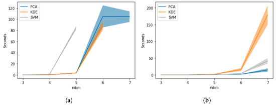
Figure 5.
Comparison of computation time in relation to number of dimensions. (a) Computation time for TPD outputs. (b) Computation time for kernel only.
Additionally, we compared the computation time to produce KDE and SVM TPD outputs when increasing the number of data points, from , , ,…, , to simulate common kernel sizes while keeping the number of dimensions at four. Figure 6 shows the mean computation time based on multiple iterations (n = 10) with the shaded area representing the standard deviation. KDE shows a higher increase in computation time with an increase in data points compared to SVM.
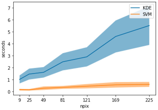
Figure 6.
Chart comparing TPD computation time between KDE and SVM in relation to the number of data points.
Next, the three approaches were implemented in a moving-window approach to be applied to the ULS dataset. The TPD outputs are presented per approach in Figure 7, Figure 8, Figure 9 and Figure 10.

Figure 7.
KDE functional diversity maps with , , and in their own figure.

Figure 8.
SVM functional diversity maps with , , and in their own figure.

Figure 9.
PCA, from four traits, functional diversity maps with , , and in their own figure.

Figure 10.
PCA, from nine traits, functional diversity maps with , , and in their own figure.
Figure 7, Figure 8, Figure 9 and Figure 10 show functional diversity maps computed for the three different approaches. Computation time of the KDE images was 19 min, and SVM took 18 min to compute. Figure 9 and Figure 10 were produced with the PCA approach, one with the four selected traits and the other one with all nine original traits. Both PCA maps used three components. The first calculation took 9 min and explained 92% of the variance, while the second took 14 min and explained 87% of the variance.
The maps have proportionally more bright areas compared to the and maps. Comparing the close-up images, it is clear that areas with high have low and , while high and values seem to occur together. Some of these observation might correlate to areas with rapid change of presence of vegetation or lack thereof. Comparing Figure 7a to the study site in Figure 1, high can be observed on the edge of the canopy of large trees, while is low in the centre of these trees. maps show geometric artefacts, which is consistent with the patterns from other studies [26]. These artefacts occur along the edges of canopies where is high.
The SVM map (Figure 8) shows clearly different patterns in the distribution of the traits when compared to the KDE map, and is not directly comparable. Areas of high are continuous with a clear edge, separating them from the other areas. While similar patterns can be clearly observed in the image, these artefacts are particularly noticeable in the maps from the SVM results.
Comparing the effect of PCA in the FD maps, Figure 9 looks similar to the KDE images in Figure 7 with only sight changes in brightness. However, comparing the close-up of Figure 9, showing PCA results based on four traits, to Figure 10, showing PCA results based on nine traits, shows subtle differences in FD patterns. PCA from nine traits reduces the proportion of high and values compared to PCA from four traits.
4. Discussion
4.1. Selection of Traits
The main trait selection factor was the suitability of published variables based on the five criteria outlined at the beginning of Section 2.3. The second selection factor was the recommendation by Valbuena et al. [6] to use a standardised framework of traits describing canopy height, cover, and structural complexity, which allows for comparison with results of previous studies, e.g., Schneider et al. [37]. The selection process resulted in nine morphological traits that met the above-outlined criteria, from which we used four core traits selected based on statistical analysis. In our experience, the available size of computer RAM is one of the potential limiting factors when employing a high number of traits for mapping FD without the capability of employing out-of-memory techniques. Although scaling solutions such as Dask for Python [86] have the potential to reduce the memory requirements, we decided to limit our approach to only four core traits to lower TPD computational demands and hardware requirements when constructing the trait space in the hypervolume. The selection of core traits makes our method faster, more operational, less complex, and, therefore, usable by a broader scientific community.
The four core traits are , , , and . was selected for the ecological reasons outlined in Section 2.3. We selected over because of a higher correlation between TLS and ULS results; however, the regression statistical indicators did not point out a clear interpretation advantage of either one. The technical advantages of are its ability to produce fewer empty cells in the grid layer and its intuitive use, as high values indicate greater vertical structural variability. This relationship in the case of is negative [59]. Given the similarity in calculation and the fact that has been proven to be ecologically significant, we assume that has equal ability to predict ecosystem services [26,60,67].
was found to have a higher PCA loading compared to and , which is why it was selected as a core trait. However, the implementation of depends on the number of lidar return points. Therefore, the lidar sensor type and platform have an influence on the performance. Our implementation was based on the number of classified ground points instead of returns because the number of return points between ULS and TLS was inconsistent due to the different viewing angles. Another recent study Jiang et al. [77] used Beer’s law to estimate leaf area index from aerial full-waveform lidar data, which offers future avenues for our follow-up research.
is a relatively new variable that we found to be consistent between ULS and TLS platforms, as well as across different grid sizes. is based on space voxelisation and, therefore, captures three-dimensional structural complexity of an investigated canopy. , selected because of its statistical performance, is the only trait that captures the whole three-dimensional space, making it a novel addition.
Although had a consistently high PCA loading, independent of other variables, and was capable of explaining a large portion of the variation in the data that was not captured by other traits, it was not selected due to the lack of clear ecological meaning and poor relative performance in the regression and PCA. A similar performance was found in other studies, e.g., Schneider et al. [37], but no causal factor for the ecological significance of is evidenced in the published literature. Yet, it might be a suitable candidate, especially in future studies encompassing structurally different forest environments.
4.2. Comparison between TLS- and ULS-Derived Traits
TLS and ULS have inherent differences that we attempted to minimise through voxelisation of the TLS point clouds. However, the different viewing directions and levels of occlusion of both systems (TLS from the ground up and ULS from the top down) cannot be fully compensated and result in an uneven spread of point density through the vertical column of the forest canopy. Object occlusion in a TLS point cloud results in lack of details on the upper canopy, while an ULS point cloud lacks detailed characterisation of the understorey vegetation.
Since our selection was focused on traits that were consistent for both techniques, the traits that were not selected (i.e., , R, , and ) might give us some additional insight into the differences between TLS and ULS approaches. As discussed in Section 4.1, and might be more suitable for products of aerial full-waveform lidar systems. Our implementation of had to be adjusted to use ground-classified points. relies on the relative height ratio, which is based on the 98th and 25th percentile. These are likely to be different between TLS and ULS due to differences in point density distribution within the vertical column and, therefore, are inconsistent between the two techniques. Finally, R, based on the standard deviation of the canopy height, is likely to differ since TLS acquisitions are impacted by more frequent object occlusion in the upper parts of the scanned canopy than its ULS acquisitions. The consistency and accuracy between traits-derived ULS and TLS can be improved by using TLS as a local calibration tool for ULS [87].
4.3. Trait Probability Density Approach Comparison
Comparison of KDE, PCA, and SVM approaches revealed their advantages and disadvantages. In all approaches, the values declined with an increasing number of traits. This is expected because increasing number of traits is also increasing the space within the hypervolume, while the number of data points remains constant. However, based on SVM started at much higher values and dropped noticeably with an increasing number of traits, while both KDE and PCA showed only a slight decline. Hence, the hypervolume derived from SVM is seemingly more sensitive with an increasing number of traits. In our tests, adjusting and parameters of SVM had the strongest impact on values.
was gaining values close to five for all approaches and all tested traits. The artificial dataset is most likely regularly distributed, resulting in a low evenness, and an increase in the hypervolume decreases the evenness even further.
The value of stabilises at a very small value with four or more traits for any of the three approaches. KDE- and PCA-based are almost identical and started higher than SVM, indicating the initial divergence of the dataset. SVM, on the contrary, failed to capture this divergence.
Computation time of , , and for each approach increases significantly for an increasing number of traits. While SVM was found to be unsuitable for computing TPD in high-dimensional hypervolumes, PCA was able to calculate FD output for one more additional trait in comparison to KDE. However, this computation depends on the correlation between traits in the dataset, and PCA might encompass more additional traits when applied to real-world data. PCA has the potential to reduce memory requirements by reducing the number of dimensions. Comparing the computation time for different kernel sizes only, SVM speed was similar to PCA, but it was faster than KDE. This indicates that, except for the FD calculation, SVM might have some benefits over KDE when working with a high-dimensional hypervolume.
4.4. Kernel Size
In the context of TPD computation, the kernel size was determined based on two considerations: (i) its mathematical validity and (ii) a spatial extent of the investigated ecological unit. For KDE, Blonder et al. [84] recommends that the ratio between kernel size and number of traits should not be below 10. We adopted these recommendations and calculated TPD for kernel sizes of pixels for 3–5 traits. These kernel sizes, in combination with the number of traits, provided sufficient data points for KDE to produce a mathematically valid result, although some previous studies ignored these recommendations and used a kernel [26,37]. Table A22 in the Appendix B provides an overview of the minimum recommended kernel sizes in relation to the number of traits.
The second consideration relates to the ecological unit under the functional diversity assessment. Once the size of the kernel is set, the pixel spatial resolution must be appropriately sized to capture sufficient details of the desired ecological unit to which the TPD approach is applied. In our study, focusing on forest canopy elements of dominant trees, high-point-density data enabled us to cover the appropriate spatial extent with a kernel size of at a pixel size of .
4.5. Functional Diversity Maps
It has been shown that other environmental factors, such as soil type, have a strong influence on [26,37]. Therefore, interpretation of FD maps might benefit from ancillary information provided by environmental, topographic, and soil maps or from other existing FD maps. Although a single FD map has a limited explanatory power, one can relate some of its informational content to the actual forest structure. For instance, areas with high in red colour are related to a fully occupied vertical column in the forest. Towards the edges of these areas, one can find high in blue colour that might indicate a change or transition in distribution of forest elements occupying space within the vertical column. Finally, the cyan-coloured areas indicate presence of only little vegetation, such as a low-stature understorey. As stated in Section 2.1, Australian forests are occasionally impacted by wildfires that modify their forest structure. After a fire reduction of the under- and mid-storey layers, the cyan-coloured areas are likely to expand because high values represent a canopy dominated by stems of large trees. During the post-burning recovery phase, one expects that new areas with high start to emerge, and they transition over time to high (red colours). FD maps have the potential to evaluate differences in functional diversity among larger geographical areas. Nevertheless, intercomparison of FD maps is only possible when all maps are based on the same traits, TPD approach, and kernel size. Such a standardised approach can facilitate regular monitoring of functional diversity over time, such as in the example of bushfire recovery monitoring suggested in this section.
5. Conclusions
In this paper, we investigated the role of trait dimensionality in the TPD approach by comparing different techniques for quantifying hypervolumes and methods to reduce the data dimensionality. These approaches were tested on morphological traits derived from high-point-density lidar data of Australian forest canopies collected with UAS and TLS systems. Our study expanded the knowledge on the existing workflow established by Schneider et al. [26] by assessing functional diversity from multi-trait TPD in the context of lidar remote sensing observations. We identified the following functional traits to be ecologically meaningful and statically sound, while maintaining relative consistency in traits derived from ULS and TLS data: canopy height, effective number of canopy layers, plant–groundratio, and box dimensions. We compared three different methods for calculating TPD in a high-dimensional hypervolume from the morphological forest traits. The outcomes revealed that an optimal selection of morphological canopy traits combined with the principal component analysis and an appropriate kernel density calculation resulted in the most efficient functional diversity estimation. This approach provided consistent results for a varying number of traits and tested spatial resolutions in a remote sensing context. Yet, we would like to highlight the importance of the relationship between the kernel size and the number of traits for producing statisticallyrobust and scientifically sound functional diversity maps. In our research, we learned that trait selection plays an important role when assessing functional diversity at different spatial scales from data acquired by different lidar systems, and we formulated our most important findings in the set of recommendations.
- Only ecologically and statisticallysound traits are advised to be included.
- If five or more traits are selected, PCA transformation should be applied. No more than four PCA components retaining 80–95% of variance explained should be used.
- KDE is computationally more efficient than SVM and, therefore, recommended for computing TPD.
- The kernel must have a size suitable to capture the ecological target unit; however, it should be of at least when using 3–5 traits.
- Depending on the kernel size, collected data should have a pixel spatial resolution capable of capturing required spatial details of the targeted ecological unit.
The results and recommendations concluded from this work are expected to support the research effort for global monitoring of functional vegetation diversity through remote sensing by improving the quality of functional biodiversity spatial assessments.
Author Contributions
A.L. and S.P. secured funding for the project; A.L. conceived the ideas; L.H. and A.L. designed the methodology; A.L. and L.H. collected the data; L.H., A.L. and A.P.R.-B. prepared the data; B.M., L.H. and A.L. wrote the code; L.H. and A.L. analysed the data; L.H., A.L. and Z.M. led the writing of the manuscript. All authors contributed critically to the manuscript drafts and gave final approval for publication. All authors have read and agreed to the published version of the manuscript.
Funding
This research was partially funded by the Australian Government through the Australian Research Council’s Discovery Projects funding scheme (project DP180103460).
Data Availability Statement
Data will be made openly available through TERN Data Discovery Portal in accordance with the TERN terms of use. A DOI for the data will be available.
Acknowledgments
This work is supported by the use of Terrestrial Ecosystem Research Network (TERN) infrastructure and funding, which is enabled by the Australian Government’s National Collaborative Research Infrastructure Strategy (NCRIS). The authors would like to thank Will Woodgate, Emiliano Cimoli, and Juliane Bendig for their support.
Conflicts of Interest
The authors declare no conflict of interest.
Appendix A. Statistical Analysis
Appendix A.1. Grid Size 0.5 m
Appendix A.1.1. Plot Data at 0.5 m Grid Size
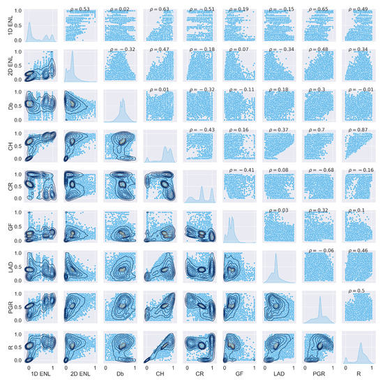
Figure A1.
Scatterplot matrix of ULS traits at 0.5 m grid size.
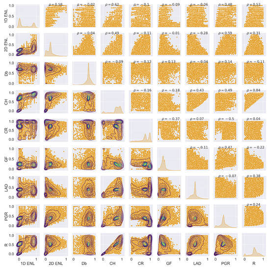
Figure A2.
Scatterplot matrix of TLS traits at 0.5 m grid size.
Appendix A.1.2. Correlation at 0.5 m Grid Size
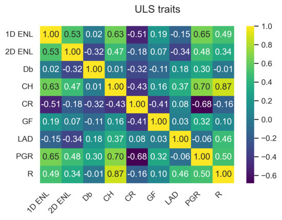
Figure A3.
ULS correlation matrix at 0.5 m grid size.
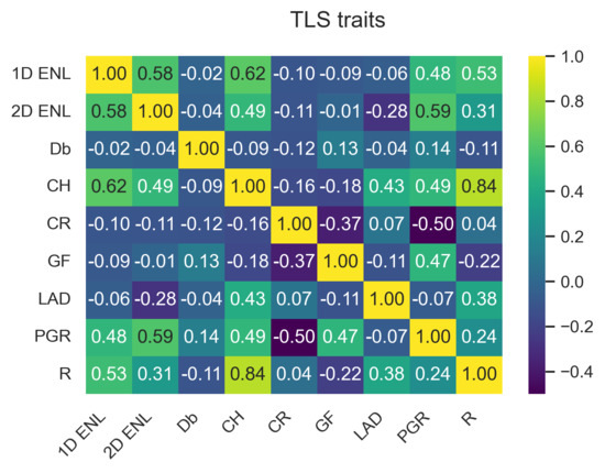
Figure A4.
TLS correlation matrix at 0.5 m grid size.

Table A1.
Overview of correlation between ULS and TLS traits at 0.5 m grid size.
Table A1.
Overview of correlation between ULS and TLS traits at 0.5 m grid size.
| Trait | Correlation |
|---|---|
| 0.600701 | |
| 0.347168 | |
| 0.157310 | |
| 0.446589 | |
| 0.043564 | |
| 0.166342 | |
| 0.165330 | |
| 0.226489 | |
| R | 0.330439 |
Appendix A.1.3. Wilcoxon Test at 0.5 m Grid Size

Table A2.
Overview of Wilcoxon test results at 0.5 m grid size.
Table A2.
Overview of Wilcoxon test results at 0.5 m grid size.
| Trait | W | p-Value |
|---|---|---|
| 0 | ||
| 0 | ||
| 0 | ||
| 0.0241798 | ||
| 0.163594 | ||
| 0 | ||
| R |
Appendix A.1.4. Linear Regression at 0.5 m Grid Size

Table A3.
Overview of ULS linear regression at 0.5 m grid size.
Table A3.
Overview of ULS linear regression at 0.5 m grid size.
| X | Y | A | B | R2 | RMSE |
|---|---|---|---|---|---|
| 0.215091 | 0.127912 | 0.279958 | 0.131094 | ||
| 0.00752914 | 0.576217 | 0.000390069 | 0.144851 | ||
| 0.429321 | 0.522204 | 0.399033 | 0.200232 | ||
| −0.436834 | 0.745498 | 0.263619 | 0.277466 | ||
| 0.065624 | 0.20423 | 0.0380166 | 0.125456 | ||
| −0.0654678 | 0.398805 | 0.0220413 | 0.16573 | ||
| 0.345233 | 0.410379 | 0.419777 | 0.154252 | ||
| R | 0.301955 | 0.448956 | 0.243971 | 0.20201 | |
| −0.300517 | 0.641774 | 0.102692 | 0.137239 | ||
| 0.780059 | 0.520697 | 0.217695 | 0.228453 | ||
| −0.385628 | 0.661853 | 0.0339492 | 0.317803 | ||
| 0.0544472 | 0.217523 | 0.00432463 | 0.127634 | ||
| −0.374048 | 0.452281 | 0.118901 | 0.157309 | ||
| 0.626913 | 0.409242 | 0.228749 | 0.177841 | ||
| R | 0.507538 | 0.456474 | 0.113905 | 0.218697 | |
| 0.023127 | 0.670128 | 0.000168282 | 0.258269 | ||
| −0.714061 | 0.994834 | 0.102368 | 0.306343 | ||
| −0.0953114 | 0.284078 | 0.0116544 | 0.127163 | ||
| 0.205753 | 0.255065 | 0.031639 | 0.164915 | ||
| 0.424685 | 0.294186 | 0.0923166 | 0.19293 | ||
| R | −0.0225023 | 0.575443 | 0.000196907 | 0.232306 | |
| −0.536924 | 0.948358 | 0.183961 | 0.292088 | ||
| 0.0802974 | 0.174003 | 0.026291 | 0.126218 | ||
| 0.237826 | 0.211647 | 0.134355 | 0.155923 | ||
| 0.547531 | 0.16585 | 0.487717 | 0.14494 | ||
| R | 0.786997 | 0.0244859 | 0.76552 | 0.112501 | |
| −0.161387 | 0.322712 | 0.166434 | 0.116782 | ||
| 0.039433 | 0.351281 | 0.00578838 | 0.167101 | ||
| −0.427951 | 0.788892 | 0.466916 | 0.147853 | ||
| R | −0.113494 | 0.628395 | 0.0249493 | 0.229412 | |
| 0.0394476 | 0.365176 | 0.000906514 | 0.167511 | ||
| 0.508362 | 0.42374 | 0.103108 | 0.19178 | ||
| R | 0.187975 | 0.519388 | 0.0107104 | 0.231081 | |
| −0.0732528 | 0.56751 | 0.00367505 | 0.202131 | ||
| R | 0.640295 | 0.322811 | 0.213322 | 0.206064 | |
| R | 0.569222 | 0.254978 | 0.246163 | 0.201717 |

Table A4.
Overview of TLS linear regression at 0.5 m grid size.
Table A4.
Overview of TLS linear regression at 0.5 m grid size.
| X | Y | A | B | R2 | RMSE |
|---|---|---|---|---|---|
| 0.259072 | 0.125031 | 0.330936 | 0.133259 | ||
| −0.00767013 | 0.70368 | 0.000547971 | 0.1185 | ||
| 0.430284 | 0.546475 | 0.379723 | 0.198943 | ||
| −0.0686811 | 0.753639 | 0.00926953 | 0.256863 | ||
| −0.031123 | 0.245778 | 0.00772719 | 0.127585 | ||
| −0.0271697 | 0.385896 | 0.00353271 | 0.165074 | ||
| 0.238619 | 0.296743 | 0.233342 | 0.156468 | ||
| R | 0.337549 | 0.407016 | 0.284584 | 0.193609 | |
| −0.0323939 | 0.708001 | 0.00198233 | 0.118415 | ||
| 0.760602 | 0.538919 | 0.24064 | 0.22012 | ||
| −0.177999 | 0.767424 | 0.0126274 | 0.256427 | ||
| −0.0113033 | 0.236609 | 0.00020671 | 0.128068 | ||
| −0.285755 | 0.439214 | 0.0792541 | 0.158678 | ||
| 0.644431 | 0.243069 | 0.345168 | 0.144607 | ||
| R | 0.430607 | 0.438001 | 0.0939279 | 0.217885 | |
| −0.1963 | 0.845548 | 0.00848485 | 0.251528 | ||
| −0.250691 | 0.903544 | 0.0132589 | 0.256345 | ||
| 0.136055 | 0.138749 | 0.0158538 | 0.127062 | ||
| −0.0500356 | 0.410763 | 0.0012863 | 0.16526 | ||
| 0.213243 | 0.236868 | 0.0200068 | 0.176903 | ||
| R | −0.204117 | 0.676759 | 0.0111723 | 0.227618 | |
| −0.159323 | 0.840657 | 0.0243211 | 0.254904 | ||
| −0.0899681 | 0.297792 | 0.0314831 | 0.126049 | ||
| 0.278758 | 0.178343 | 0.181315 | 0.149625 | ||
| 0.34654 | 0.140965 | 0.239956 | 0.155791 | ||
| R | 0.760947 | −0.0050223 | 0.705162 | 0.124291 | |
| −0.184106 | 0.3681 | 0.137598 | 0.118943 | ||
| 0.0479266 | 0.340814 | 0.0055938 | 0.164903 | ||
| −0.345989 | 0.63814 | 0.249645 | 0.154795 | ||
| R | 0.0390485 | 0.505292 | 0.00193804 | 0.228678 | |
| −0.14807 | 0.410361 | 0.0131526 | 0.164275 | ||
| 0.662696 | 0.231174 | 0.225607 | 0.157255 | ||
| R | −0.396077 | 0.626434 | 0.0491176 | 0.223208 | |
| −0.0765121 | 0.415054 | 0.00501308 | 0.178251 | ||
| R | 0.530108 | 0.334553 | 0.146666 | 0.211449 | |
| R | 0.305275 | 0.415783 | 0.0567985 | 0.222305 |

Table A5.
Overview linear regression between TLS and ULS at 0.5 m grid size.
Table A5.
Overview linear regression between TLS and ULS at 0.5 m grid size.
| Trait | A | B | R2 | RMSE |
|---|---|---|---|---|
| 0.631066 | 0.138877 | 0.360842 | 0.303833 | |
| 0.329217 | 0.135556 | 0.120525 | 0.144883 | |
| 0.192276 | 0.444299 | 0.0247464 | 0.143075 | |
| 0.456647 | 0.360222 | 0.199442 | 0.231103 | |
| 0.0545837 | 0.541631 | 0.00189782 | 0.323032 | |
| 0.16612 | 0.19 | 0.0276696 | 0.126129 | |
| 0.16755 | 0.311257 | 0.0273339 | 0.165281 | |
| 0.256659 | 0.440949 | 0.0512973 | 0.197241 | |
| R | 0.335388 | 0.383412 | 0.10919 | 0.219278 |
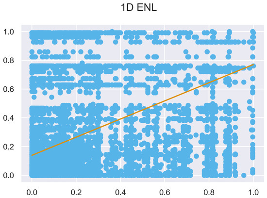
Figure A5.
ULS and TLS regression at 0.5 m grid size.
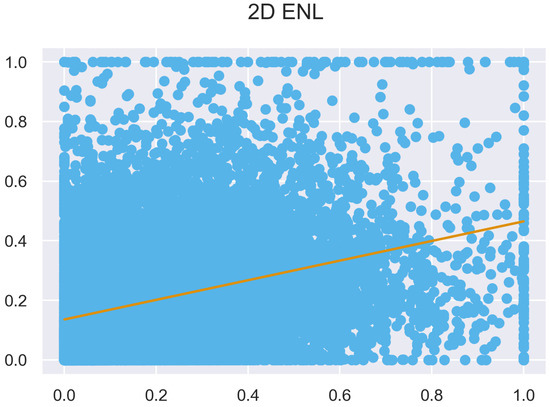
Figure A6.
ULS and TLS regression at 0.5 m grid size.
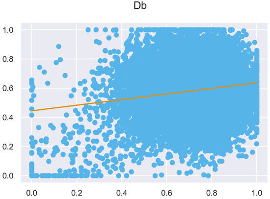
Figure A7.
ULS and TLS regression at 0.5 m grid size.
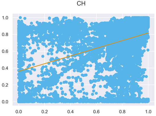
Figure A8.
ULS and TLS regression at 0.5 m grid size.
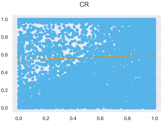
Figure A9.
ULS and TLS regression at 0.5 m grid size.
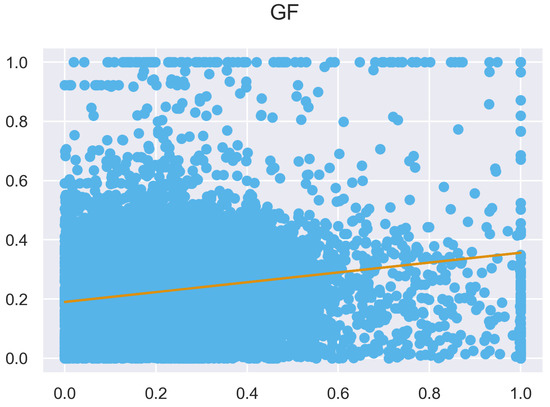
Figure A10.
ULS and TLS regression at 0.5 m grid size.
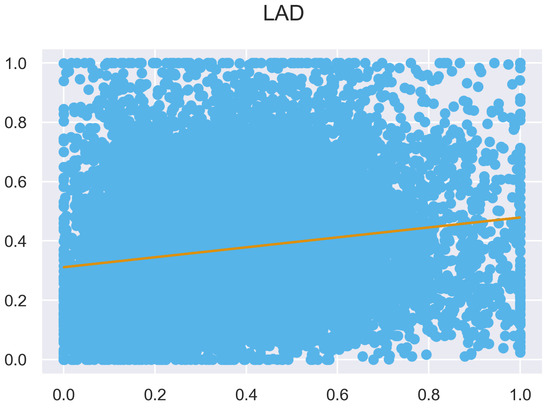
Figure A11.
ULS and TLS regression at 0.5 m grid size.
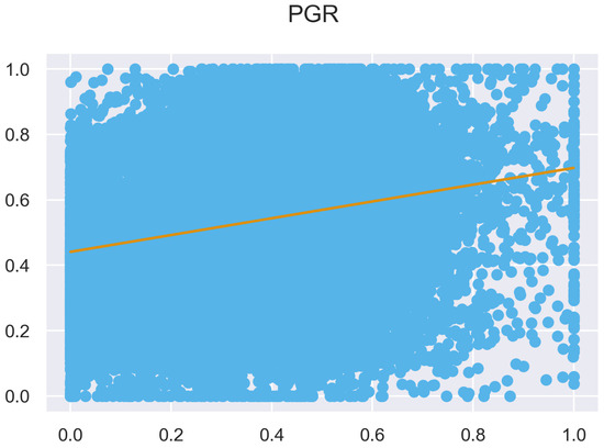
Figure A12.
ULS and TLS regression at 0.5 m grid size.
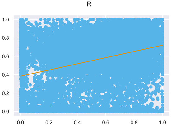
Figure A13.
ULS and TLS R regression at 0.5 m grid size.
Appendix A.1.5. PCA
Band Variation Explained at 0.5 m Grid Size

Table A6.
ULS PCA band variation explained at 0.5 m grid size.
Table A6.
ULS PCA band variation explained at 0.5 m grid size.
| Band | Variation Explained |
|---|---|
| 1 | 0.55757726 |
| 2 | 0.17158204 |
| 3 | 0.12415327 |
| 4 | 0.05240734 |
| 5 | 0.03968954 |
| 6 | 0.02471443 |
| 7 | 0.01389153 |
| 8 | 0.01045981 |
| 9 | 0.00552477 |

Table A7.
TLS PCA band variation explained at 0.5 m grid size.
Table A7.
TLS PCA band variation explained at 0.5 m grid size.
| Band | Variation Explained |
|---|---|
| 1 | 0.49571507 |
| 2 | 0.1903597 |
| 3 | 0.1373346 |
| 4 | 0.05582574 |
| 5 | 0.04323816 |
| 6 | 0.03034304 |
| 7 | 0.0284349 |
| 8 | 0.01131899 |
| 9 | 0.0074298 |
PCA Loadings at 0.5 m Grid Size
PCA Band 1 vs. PCA Band 2
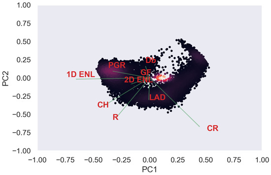
Figure A14.
ULS PCA band 1 and 2 loadings at 0.5 m grid size.
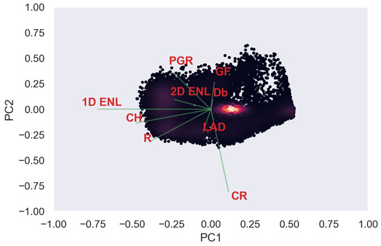
Figure A15.
TLS PCA band 1 and 2 loadings at 0.5 m grid size.
PCA Band 1 vs. PCA Band 3
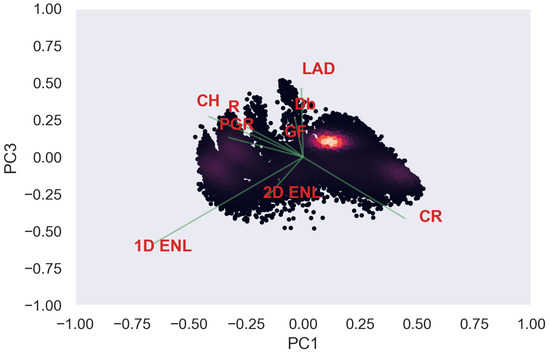
Figure A16.
ULS PCA band 1 and 3 loadings at 0.5 m grid size.
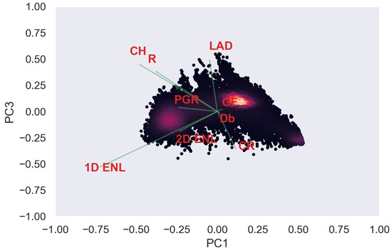
Figure A17.
TLS PCA band 1 and 3 loadings at 0.5 m grid size.
PCA Band 2 vs. PCA Band 3
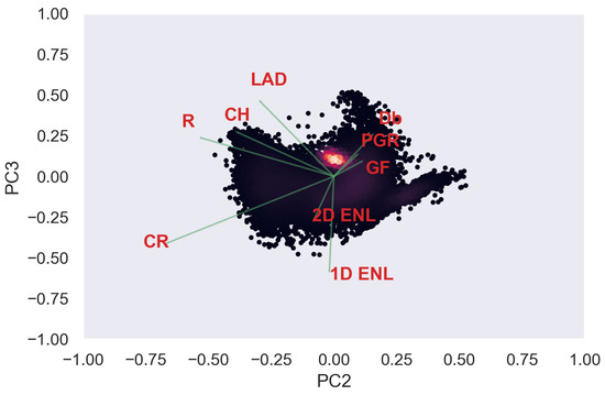
Figure A18.
ULS PCA band 2 and 3 loadings at 0.5 m grid size.
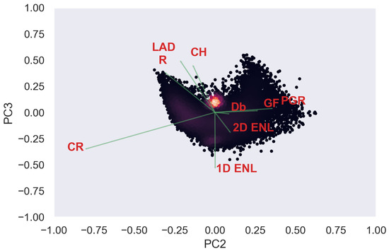
Figure A19.
TLS PCA band 2 and 3 loadings at 0.5 m grid size.
Appendix A.2. Grid Size 1 m
Appendix A.2.1. Plot Data at 1 m Grid Size
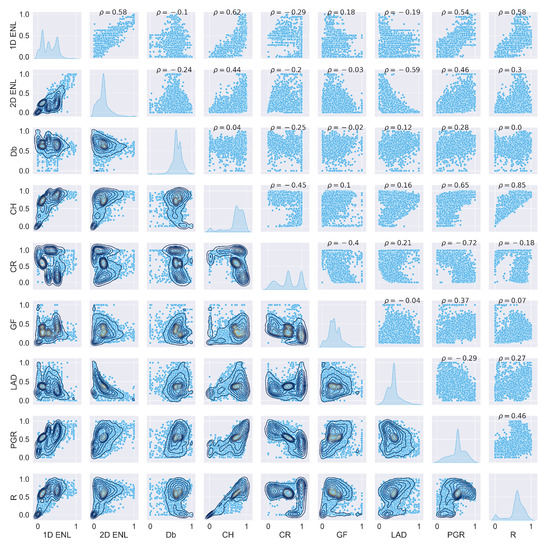
Figure A20.
ULS traits plot at 1 grid size.
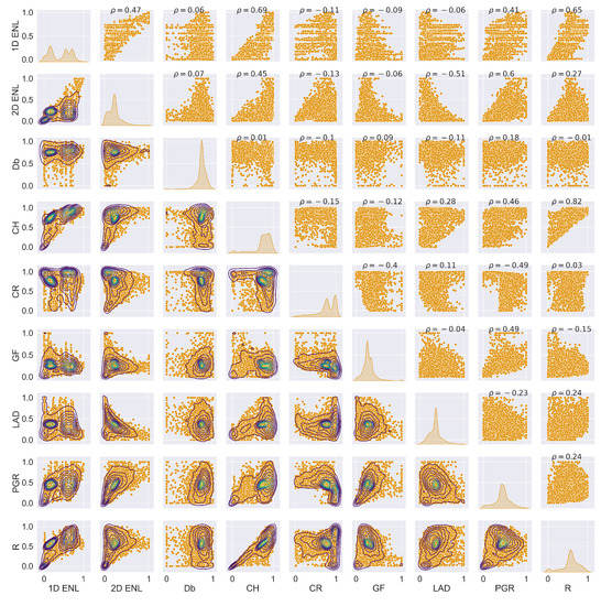
Figure A21.
TLS traits plot at 1 grid size.
Appendix A.2.2. Correlation at 1 m Grid Size
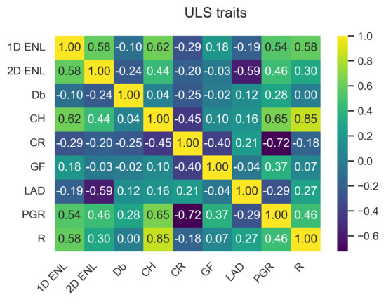
Figure A22.
ULS correlation matrix at 1 Grid Size.
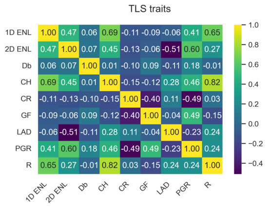
Figure A23.
TLS correlation matrix at 1 grid size.

Table A8.
Overview of correlation between ULS and TLS traits at 1 grid size.
Table A8.
Overview of correlation between ULS and TLS traits at 1 grid size.
| Trait | Correlation |
|---|---|
| 0.512485 | |
| 0.375147 | |
| 0.366927 | |
| 0.459784 | |
| 0.056302 | |
| 0.194438 | |
| 0.258495 | |
| 0.251410 | |
| R | 0.344600 |
Appendix A.2.3. Wilcoxon Test at 1 m Grid Size

Table A9.
Overview of Wilcoxon test results.
Table A9.
Overview of Wilcoxon test results.
| Trait | W | p-Value |
|---|---|---|
| 0 | ||
| 0 | ||
| R |
Appendix A.2.4. Linear regression at 1 m Grid Size

Table A10.
Overview of ULS linear regression at 1 grid size.
Table A10.
Overview of ULS linear regression at 1 grid size.
| X | Y | A | B | R2 | RMSE |
|---|---|---|---|---|---|
| 0.467729 | 0.0947887 | 0.340486 | 0.127027 | ||
| −0.0621398 | 0.669698 | 0.00946625 | 0.124038 | ||
| 0.730883 | 0.506278 | 0.386128 | 0.179829 | ||
| −0.481101 | 0.740093 | 0.0849908 | 0.308036 | ||
| 0.154704 | 0.268928 | 0.033806 | 0.161389 | ||
| −0.162501 | 0.4156 | 0.0372604 | 0.161185 | ||
| 0.566854 | 0.374242 | 0.293265 | 0.171715 | ||
| R | 0.660615 | 0.397958 | 0.340663 | 0.17934 | |
| −0.193229 | 0.696488 | 0.0588132 | 0.120909 | ||
| 0.645399 | 0.573841 | 0.193456 | 0.206127 | ||
| −0.416891 | 0.693752 | 0.0410046 | 0.315353 | ||
| −0.0287867 | 0.322121 | 0.000752087 | 0.164127 | ||
| −0.622579 | 0.513234 | 0.351411 | 0.132299 | ||
| 0.598479 | 0.403615 | 0.210041 | 0.181544 | ||
| R | 0.426143 | 0.495992 | 0.0910812 | 0.210565 | |
| 0.069692 | 0.680232 | 0.00143207 | 0.229356 | ||
| −0.652681 | 1.02065 | 0.0638061 | 0.311582 | ||
| −0.0199772 | 0.328358 | 0.000229945 | 0.164169 | ||
| 0.163487 | 0.260398 | 0.0153838 | 0.163006 | ||
| 0.457629 | 0.246407 | 0.0779661 | 0.196134 | ||
| R | 0.0076009 | 0.59125 | 0.220862 | ||
| −0.62853 | 1.05179 | 0.200685 | 0.287904 | ||
| 0.0681929 | 0.265871 | 0.00908731 | 0.163441 | ||
| 0.114343 | 0.283868 | 0.0255223 | 0.162165 | ||
| 0.582686 | 0.121546 | 0.428698 | 0.154388 | ||
| R | 0.814887 | 0.00491185 | 0.717114 | 0.117471 | |
| −0.20602 | 0.438083 | 0.163272 | 0.150188 | ||
| 0.108882 | 0.301973 | 0.0455565 | 0.160489 | ||
| −0.45979 | 0.818253 | 0.525457 | 0.140708 | ||
| R | −0.120884 | 0.668212 | 0.0310647 | 0.217406 | |
| −0.0402142 | 0.379518 | 0.00161548 | 0.164142 | ||
| 0.4563 | 0.400451 | 0.134532 | 0.190023 | ||
| R | 0.0937216 | 0.566643 | 0.00485417 | 0.220327 | |
| −0.361848 | 0.677085 | 0.0846905 | 0.195418 | ||
| R | 0.360919 | 0.4638 | 0.0720629 | 0.212757 | |
| R | 0.496437 | 0.325965 | 0.210785 | 0.19621 |

Table A11.
Overview of TLS linear regression at 1 grid size.
Table A11.
Overview of TLS linear regression at 1 grid size.
| X | Y | A | B | R2 | RMSE |
|---|---|---|---|---|---|
| 0.281689 | 0.107886 | 0.221273 | 0.139089 | ||
| 0.026867 | 0.742788 | 0.00367964 | 0.116362 | ||
| 0.592721 | 0.503637 | 0.475236 | 0.163935 | ||
| −0.0953368 | 0.800507 | 0.0112191 | 0.235573 | ||
| −0.0428402 | 0.291535 | 0.00758217 | 0.129002 | ||
| −0.0347705 | 0.37516 | 0.00329043 | 0.159281 | ||
| 0.285339 | 0.329269 | 0.169482 | 0.166253 | ||
| R | 0.54105 | 0.349931 | 0.427036 | 0.164954 | |
| 0.054596 | 0.741597 | 0.00544875 | 0.116259 | ||
| 0.645022 | 0.602211 | 0.201822 | 0.202181 | ||
| −0.200223 | 0.806178 | 0.017745 | 0.234794 | ||
| −0.0464827 | 0.28438 | 0.003201 | 0.129286 | ||
| −0.515506 | 0.475961 | 0.259363 | 0.137304 | ||
| 0.694087 | 0.291135 | 0.359617 | 0.145987 | ||
| R | 0.367182 | 0.48936 | 0.0705286 | 0.210096 | |
| 0.0253144 | 0.727056 | 0.000170051 | 0.226284 | ||
| −0.201354 | 0.913278 | 0.00981729 | 0.23574 | ||
| 0.100888 | 0.197961 | 0.008249 | 0.128959 | ||
| −0.156367 | 0.4788 | 0.0130543 | 0.158499 | ||
| 0.278007 | 0.236454 | 0.0315607 | 0.179527 | ||
| R | −0.0180399 | 0.584889 | 0.217911 | ||
| −0.162112 | 0.88246 | 0.0239808 | 0.234048 | ||
| −0.0712072 | 0.327138 | 0.0154857 | 0.128487 | ||
| 0.196718 | 0.214156 | 0.0778593 | 0.153207 | ||
| 0.367148 | 0.172067 | 0.207431 | 0.16241 | ||
| R | 0.791223 | −0.0190701 | 0.675119 | 0.124211 | |
| −0.217696 | 0.439784 | 0.158619 | 0.118781 | ||
| 0.0770149 | 0.302287 | 0.013078 | 0.158497 | ||
| −0.373943 | 0.730768 | 0.235816 | 0.159475 | ||
| R | 0.0315358 | 0.547276 | 0.00117533 | 0.217793 | |
| −0.0546836 | 0.375918 | 0.00196994 | 0.159386 | ||
| 0.696829 | 0.255073 | 0.244659 | 0.15855 | ||
| R | −0.253531 | 0.64076 | 0.0226966 | 0.215434 | |
| −0.262925 | 0.540908 | 0.0528728 | 0.177541 | ||
| R | 0.329626 | 0.452317 | 0.0582376 | 0.21148 | |
| R | 0.281704 | 0.445648 | 0.055613 | 0.211775 |

Table A12.
Overview linear regression between TLS and ULS at 1 grid size.
Table A12.
Overview linear regression between TLS and ULS at 1 grid size.
| Trait | A | B | R2 | RMSE |
|---|---|---|---|---|
| 0.379949 | 0.144637 | 0.26264 | 0.167563 | |
| 0.372293 | 0.152076 | 0.140735 | 0.144993 | |
| 0.392272 | 0.355364 | 0.134635 | 0.115936 | |
| 0.46632 | 0.377667 | 0.211401 | 0.203821 | |
| 0.0765311 | 0.537443 | 0.00316991 | 0.321514 | |
| 0.246533 | 0.2478 | 0.0378062 | 0.161055 | |
| 0.26616 | 0.27077 | 0.0668196 | 0.158691 | |
| 0.281494 | 0.418797 | 0.063207 | 0.197698 | |
| R | 0.349254 | 0.396673 | 0.118749 | 0.207336 |
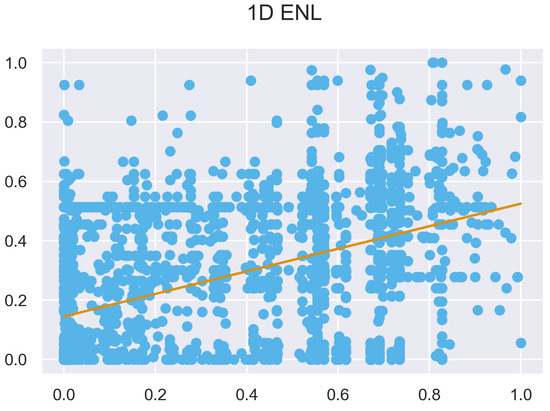
Figure A24.
ULS and TLS regression at 1 grid size.
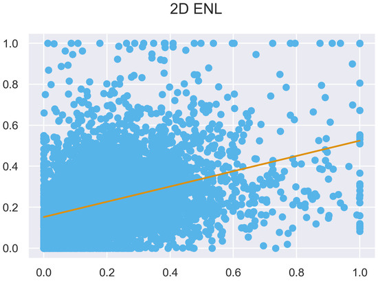
Figure A25.
ULS and TLS regression at 1 grid size.
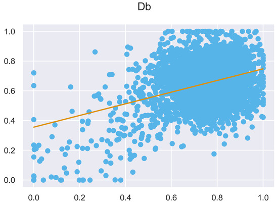
Figure A26.
ULS and TLS regression at 1 grid size.
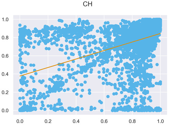
Figure A27.
ULS and TLS regression at 1 grid size.
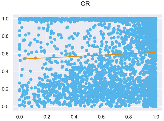
Figure A28.
ULS and TLS regression at 1 grid size.
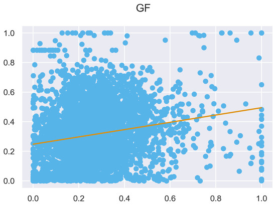
Figure A29.
ULS and TLS regression at 1 grid size.
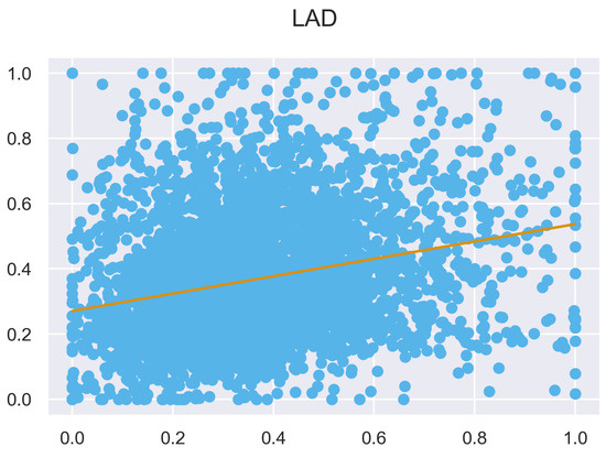
Figure A30.
ULS and TLS regression at 1 grid size.
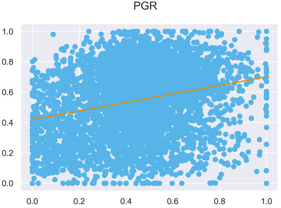
Figure A31.
ULS and TLS regression at 1 grid size.
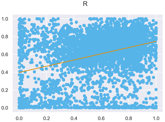
Figure A32.
ULS and TLS R regression at 1 grid size.
Appendix A.2.5. PCA at 1 m Grid Size
PCA Band Variation Explained at 1 m Grid Size

Table A13.
ULS PCA band variation explained at 1 grid size.
Table A13.
ULS PCA band variation explained at 1 grid size.
| Band | Variation Explained |
|---|---|
| 1 | 0.49122046 |
| 2 | 0.21151658 |
| 3 | 0.12150709 |
| 4 | 0.06340739 |
| 5 | 0.04095743 |
| 6 | 0.03254629 |
| 7 | 0.01713903 |
| 8 | 0.0139459 |
| 9 | 0.00775983 |

Table A14.
TLS PCA band variation explained at 1 grid size.
Table A14.
TLS PCA band variation explained at 1 grid size.
| Band | Variation Explained |
|---|---|
| 1 | 0.45179188 |
| 2 | 0.21768645 |
| 3 | 0.12141819 |
| 4 | 0.06420567 |
| 5 | 0.05201445 |
| 6 | 0.03848204 |
| 7 | 0.03369847 |
| 8 | 0.01137524 |
| 9 | 0.00932761 |
PCA Loadings at 1 m Grid Size
PCA Band 1 vs. PCA Band 2
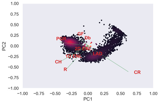
Figure A33.
ULS PCA band 1 and 2 loadings at 1 grid size.
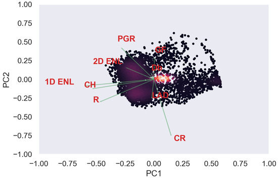
Figure A34.
TLS PCA band 1 and 2 loadings at 1 grid size.
PCA Band 1 vs. PCA Band 3
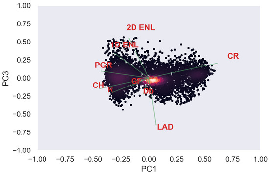
Figure A35.
ULS PCA band 1 and 3 loadings at 1 grid size.
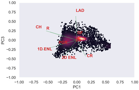
Figure A36.
TLS PCA band 1 and 3 loadings at 1 grid size.
PCA Band 2 vs. PCA Band 3
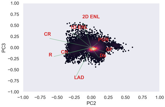
Figure A37.
ULS PCA band 2 and 3 loadings at 1 grid size.
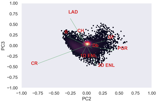
Figure A38.
TLS PCA band 2 and 3 loadings at 1 grid size.
Appendix A.3. Grid Size 5 m
Appendix A.3.1. Plot Data at 5 m Grid Size
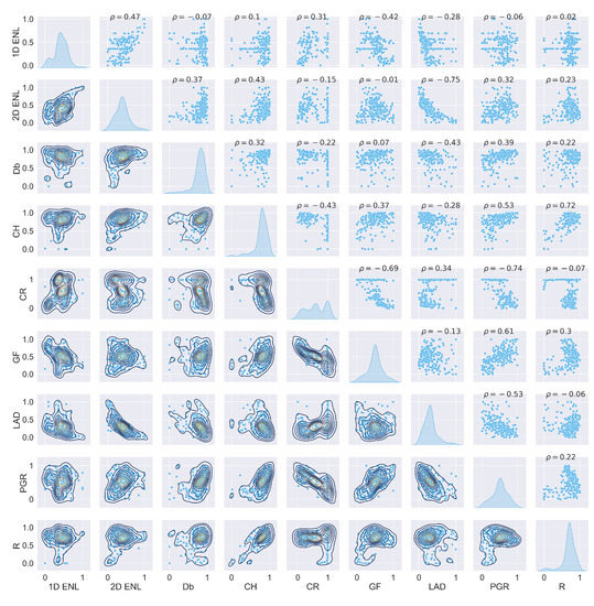
Figure A39.
ULS traits plot at 5 grid size.
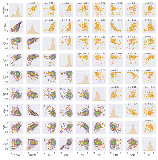
Figure A40.
TLS traits plot at 5 grid size.
Appendix A.3.2. Correlation at 5 m Grid Size
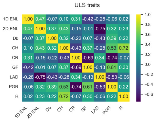
Figure A41.
ULS correlation matrix at 5 grid size.
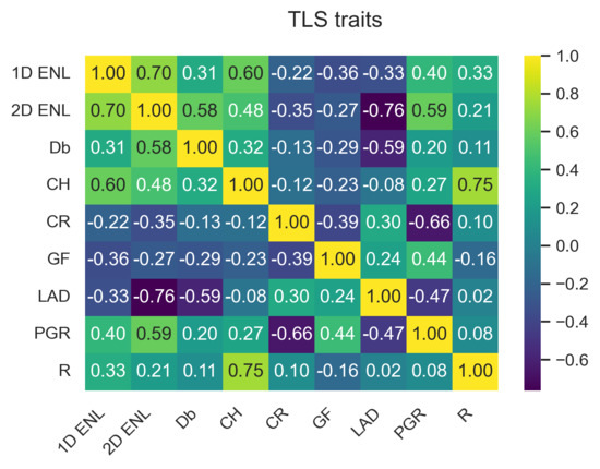
Figure A42.
TLS correlation matrix at 5 grid size.

Table A15.
Overview of correlation between ULS and TLS traits at 5 grid size.
Table A15.
Overview of correlation between ULS and TLS traits at 5 grid size.
| Trait | Correlation |
|---|---|
| 0.376877 | |
| 0.544680 | |
| 0.838943 | |
| 0.565103 | |
| 0.141271 | |
| 0.093696 | |
| 0.509761 | |
| 0.340426 | |
| R | 0.399058 |
Appendix A.3.3. Wilcoxon Test at 5 m Grid Size

Table A16.
Overview of Wilcoxon Test Results at 5 Grid Size.
Table A16.
Overview of Wilcoxon Test Results at 5 Grid Size.
| Trait | W | p-Value |
|---|---|---|
| 7960 | ||
| 16,214 | 0.000858587 | |
| 18,978 | 0.195676 | |
| 19,460 | 0.340512 | |
| 10,804 | ||
| 9913 | ||
| 19,012 | 0.144449 | |
| 15,520 | 0.000184695 | |
| R | 11,905 |
Appendix A.3.4. Linear Regression at 5 m Grid Size

Table A17.
Overview of ULS linear regression at 5 grid size.
Table A17.
Overview of ULS linear regression at 5 grid size.
| X | Y | A | B | R2 | RMSE |
|---|---|---|---|---|---|
| 0.508918 | 0.184182 | 0.224984 | 0.17066 | ||
| −0.0656667 | 0.814546 | 0.0045954 | 0.174617 | ||
| 0.100075 | 0.743007 | 0.0109168 | 0.172107 | ||
| 0.573464 | 0.365896 | 0.0978602 | 0.314589 | ||
| −0.463906 | 0.694324 | 0.176258 | 0.181198 | ||
| −0.296995 | 0.439674 | 0.0805444 | 0.181301 | ||
| −0.0715024 | 0.538589 | 0.00343391 | 0.220081 | ||
| R | 0.0234113 | 0.687707 | 0.000536352 | 0.182594 | |
| 0.335529 | 0.65312 | 0.138114 | 0.162485 | ||
| 0.382951 | 0.632519 | 0.184024 | 0.156322 | ||
| −0.255904 | 0.709564 | 0.0224333 | 0.327476 | ||
| −0.00923311 | 0.502517 | 0.199637 | |||
| −0.729762 | 0.605432 | 0.559815 | 0.125445 | ||
| 0.368356 | 0.361618 | 0.104913 | 0.208575 | ||
| R | 0.214895 | 0.611907 | 0.0520234 | 0.177829 | |
| 0.316582 | 0.536068 | 0.102514 | 0.163944 | ||
| −0.414134 | 0.933423 | 0.04789 | 0.323184 | ||
| 0.0762783 | 0.438815 | 0.00447156 | 0.199198 | ||
| −0.46905 | 0.683605 | 0.188514 | 0.170324 | ||
| 0.496537 | 0.117746 | 0.155389 | 0.202608 | ||
| R | 0.233165 | 0.514101 | 0.0499223 | 0.178026 | |
| −0.820537 | 1.25182 | 0.183801 | 0.299229 | ||
| 0.423276 | 0.166489 | 0.134615 | 0.185722 | ||
| −0.302395 | 0.551955 | 0.0766022 | 0.181689 | ||
| 0.68066 | −0.025981 | 0.285474 | 0.186354 | ||
| R | 0.764744 | 0.0971127 | 0.525034 | 0.125874 | |
| −0.416519 | 0.751892 | 0.47749 | 0.144313 | ||
| 0.192411 | 0.197622 | 0.113606 | 0.178012 | ||
| −0.492884 | 0.807911 | 0.548333 | 0.148162 | ||
| R | −0.0377769 | 0.720524 | 0.00469308 | 0.182214 | |
| 0.12478 | 0.376766 | 0.0173595 | 0.187427 | ||
| 0.672389 | 0.173047 | 0.370766 | 0.174878 | ||
| R | 0.27277 | 0.561505 | 0.0889005 | 0.174336 | |
| −0.622036 | 0.704102 | 0.284606 | 0.186467 | ||
| R | −0.05401 | 0.71456 | 0.00312616 | 0.182357 | |
| R | 0.185637 | 0.603184 | 0.0502087 | 0.177999 |

Table A18.
Overview of TLS linear regression at 5 grid size.
Table A18.
Overview of TLS linear regression at 5 grid size.
| X | Y | A | B | R2 | RMSE |
|---|---|---|---|---|---|
| 0.715746 | 0.0321566 | 0.496871 | 0.155009 | ||
| 0.252624 | 0.65337 | 0.0939562 | 0.168837 | ||
| 0.534268 | 0.485741 | 0.357961 | 0.153994 | ||
| −0.208267 | 0.901649 | 0.0464868 | 0.203002 | ||
| −0.296885 | 0.546428 | 0.127087 | 0.167457 | ||
| −0.296218 | 0.471961 | 0.109901 | 0.18143 | ||
| 0.331246 | 0.367594 | 0.158294 | 0.164391 | ||
| R | 0.319043 | 0.450987 | 0.111923 | 0.193417 | |
| 0.468106 | 0.592127 | 0.332614 | 0.144904 | ||
| 0.420108 | 0.603133 | 0.228198 | 0.16884 | ||
| −0.330458 | 0.928111 | 0.120668 | 0.194946 | ||
| −0.222023 | 0.476244 | 0.073282 | 0.172541 | ||
| −0.671223 | 0.596779 | 0.581819 | 0.124358 | ||
| 0.482919 | 0.343994 | 0.346886 | 0.144808 | ||
| R | 0.194554 | 0.54549 | 0.0429117 | 0.200792 | |
| 0.343356 | 0.512206 | 0.100422 | 0.182281 | ||
| −0.152852 | 0.906441 | 0.017008 | 0.206116 | ||
| −0.296419 | 0.615684 | 0.0860517 | 0.171348 | ||
| −0.635381 | 0.811048 | 0.343456 | 0.15582 | ||
| 0.203003 | 0.391855 | 0.0403825 | 0.175529 | ||
| R | 0.123165 | 0.531876 | 0.0113297 | 0.204078 | |
| −0.130362 | 0.887287 | 0.0145236 | 0.206377 | ||
| −0.218343 | 0.55148 | 0.0548134 | 0.174252 | ||
| −0.0794456 | 0.368332 | 0.00630381 | 0.191698 | ||
| 0.247099 | 0.35922 | 0.0702408 | 0.172776 | ||
| R | 0.805077 | −0.00232596 | 0.568305 | 0.134852 | |
| −0.332595 | 0.641111 | 0.148823 | 0.165359 | ||
| 0.276274 | 0.0890984 | 0.0892018 | 0.183528 | ||
| −0.56585 | 0.997385 | 0.431003 | 0.135162 | ||
| R | 0.102254 | 0.549523 | 0.0107274 | 0.20414 | |
| 0.257987 | 0.207908 | 0.0578161 | 0.186663 | ||
| 0.438895 | 0.386431 | 0.192734 | 0.160993 | ||
| R | −0.179731 | 0.698091 | 0.0246343 | 0.2027 | |
| −0.435111 | 0.686356 | 0.218065 | 0.158447 | ||
| R | 0.0218009 | 0.623115 | 0.000417244 | 0.205201 | |
| R | 0.0895923 | 0.58022 | 0.00611786 | 0.204615 |

Table A19.
Overview of linear regression between TLS and ULS at 5 grid size.
Table A19.
Overview of linear regression between TLS and ULS at 5 grid size.
| Trait | A | B | R2 | RMSE |
|---|---|---|---|---|
| 0.316389 | 0.244084 | 0.142036 | 0.167355 | |
| 0.483169 | 0.189293 | 0.296676 | 0.162575 | |
| 0.827804 | 0.128815 | 0.703825 | 0.0952492 | |
| 0.508846 | 0.385654 | 0.319342 | 0.142773 | |
| 0.225071 | 0.430885 | 0.0199574 | 0.32789 | |
| 0.104367 | 0.459172 | 0.00877894 | 0.198767 | |
| 0.5012 | 0.161177 | 0.259857 | 0.162665 | |
| 0.418845 | 0.27674 | 0.11589 | 0.207292 | |
| R | 0.355116 | 0.473926 | 0.159247 | 0.16747 |
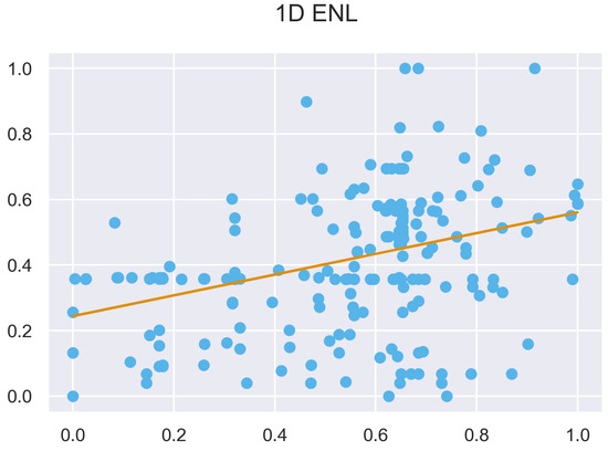
Figure A43.
ULS and TLS regression at 5 grid size.
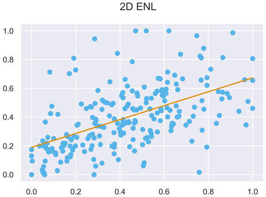
Figure A44.
ULS and TLS regression at 5 grid size.
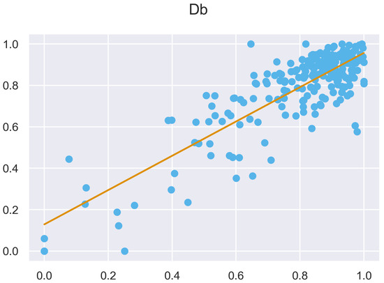
Figure A45.
ULS and TLS regression at 5 grid size.
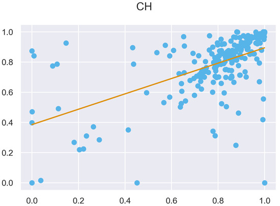
Figure A46.
ULS and TLS regression at 5 grid size.
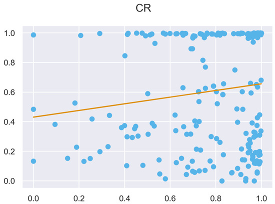
Figure A47.
ULS and TLS regression at 5 grid size.
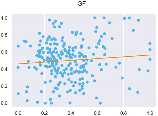
Figure A48.
ULS and TLS regression at 5 grid size.
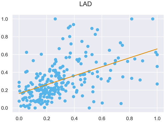
Figure A49.
ULS and TLS regression at 5 grid size.
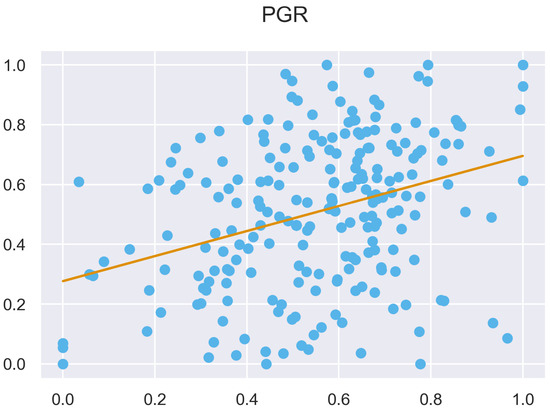
Figure A50.
ULS and TLS regression at 5 grid size.
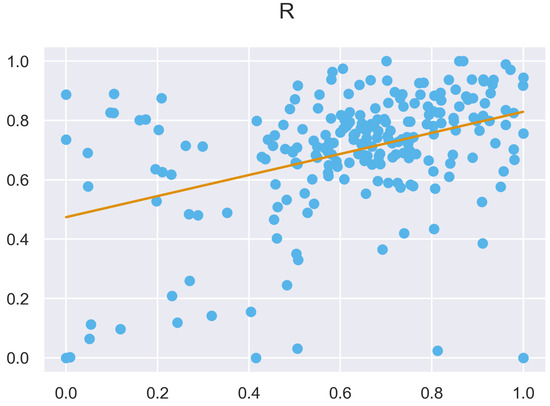
Figure A51.
ULS and TLS R regression at 5 grid size.
Appendix A.3.5. PCA at 5 m Grid Size
PCA Band Variation Explained at 5 m Grid Size

Table A20.
ULS PCA Band Variation Explained at 5 Grid Size.
Table A20.
ULS PCA Band Variation Explained at 5 Grid Size.
| Band | Variation Explained |
|---|---|
| 1 | 0.4766402 |
| 2 | 0.20790359 |
| 3 | 0.11730646 |
| 4 | 0.07081182 |
| 5 | 0.07081182 |
| 6 | 0.03822093 |
| 7 | 0.02095918 |
| 8 | 0.01562171 |
| 9 | 0.00993356 |

Table A21.
TLS PCA band variation explained at 5 grid size.
Table A21.
TLS PCA band variation explained at 5 grid size.
| Band | Variation Explained |
|---|---|
| 1 | 0.4224644 |
| 2 | 0.21853976 |
| 3 | 0.15651728 |
| 4 | 0.07522093 |
| 5 | 0.04950927 |
| 6 | 0.0383746 |
| 7 | 0.01876894 |
| 8 | 0.01192609 |
| 9 | 0.00867874 |
PCA Loadings at 5 m Grid Size
PCA Band 1 vs. PCA Band 2
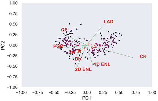
Figure A52.
ULS PCA band 1 and 2 loadings at 5 grid size.
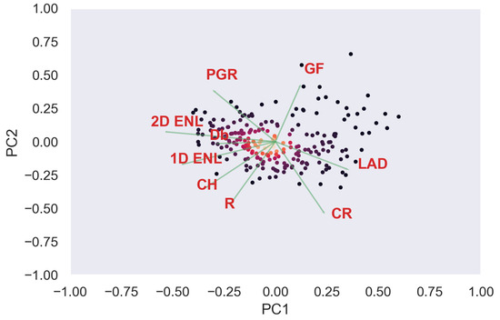
Figure A53.
TLS PCA band 1 and 2 loadings at 5 grid size.
PCA Band 1 vs. PCA Band 3
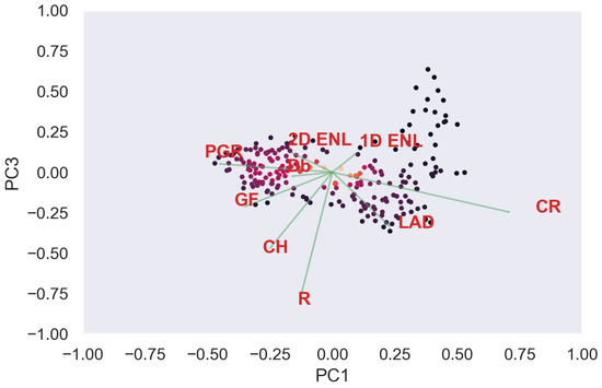
Figure A54.
ULS PCA band 1 and 3 loadings at 5 grid size.
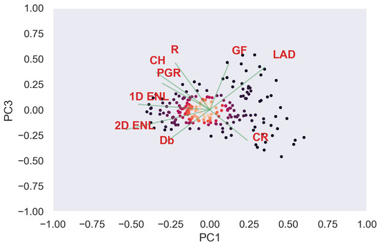
Figure A55.
TLS PCA band 1 and 3 loadings at 5 grid size.
PCA band 2 vs. PCA band 3
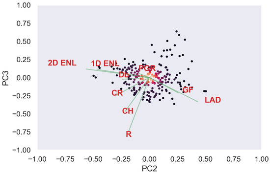
Figure A56.
ULS PCA Band 2 and 3 loadings at 5 Grid Size.
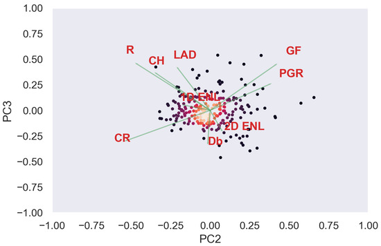
Figure A57.
TLS PCA band 2 and 3 loadings at 5 grid size.
Appendix B. Kernel Size

Table A22.
Recommended minimum kernel sizes for number of traits based on .
Table A22.
Recommended minimum kernel sizes for number of traits based on .
| Number of Traits | Recommended Minimum Kernel Size |
|---|---|
| 3 | 7 × 7 |
| 4 | 7 × 7 |
| 5 | 7 × 7 |
| 6 | 9 × 9 |
| 7 | 9 × 9 |
| 8 | 9 × 9 |
References
- Bastin, J.F.; Finegold, Y.; Garcia, C.; Mollicone, D.; Rezende, M.; Routh, D.; Zohner, C.M.; Crowther, T.W. The global tree restoration potential. Science 2019, 365, 76–79. [Google Scholar] [CrossRef] [PubMed]
- Myers, N.; Mittermeier, R.A.; Mittermeier, C.G.; Fonseca, G.A.B.d.; Kent, J. Biodiversity hotspots for conservation priorities. Nature 2000, 403, 853–858. [Google Scholar] [CrossRef] [PubMed]
- United Nations Environment Programme; Earthscan. Global Environment Outlook 3; Earthscan Publications Ltd.: London, UK, 2002. [Google Scholar]
- Pereira, H.M.; Ferrier, S.; Walters, M.; Geller, G.N.; Jongman, R.H.G.; Scholes, R.J.; Bruford, M.W.; Brummitt, N.; Butchart, S.H.M.; Cardoso, A.C.; et al. Essential Biodiversity Variables. Science 2013, 339, 277–278. [Google Scholar] [CrossRef] [PubMed]
- Skidmore, A.; Pettorelli, N.; Coops, N.; Geller, G.; Hansen, M.; Lucas, R.; Mücher, C.; O’Connor, B.; Paganini, M.; Pereira, H.; et al. Environmental science: Agree on biodiversity metrics to track from space. Nature 2015, 523, 403–405. [Google Scholar] [CrossRef] [PubMed]
- Valbuena, R.; O’Connor, B.; Zellweger, F.; Simonson, W.; Vihervaara, P.; Maltamo, M.; Silva, C.A.; Almeida, D.R.A.; Danks, F.; Morsdorf, F.; et al. Standardizing Ecosystem Morphological Traits from 3D Information Sources. Trends Ecol. Evol. 2020, 35, 656–667. [Google Scholar] [CrossRef] [PubMed]
- Migliavacca, M.; Musavi, T.; Mahecha, M.D.; Nelson, J.A.; Knauer, J.; Baldocchi, D.D.; Perez-Priego, O.; Christiansen, R.; Peters, J.; Anderson, K.; et al. The three major axes of terrestrial ecosystem function. Nature 2021, 598, 468–472. [Google Scholar] [CrossRef]
- Calders, K.; Phinn, S.; Ferrari, R.; Leon, J.; Armston, J.; Asner, G.P.; Disney, M. 3D Imaging Insights into Forests and Coral Reefs. Trends Ecol. Evol. 2019, 35, 6–9. [Google Scholar] [CrossRef]
- Cadotte, M.W.; Carscadden, K.; Mirotchnick, N. Beyond species: Functional diversity and the maintenance of ecological processes and services. J. Appl. Ecol. 2011, 48, 1079–1087. [Google Scholar] [CrossRef]
- LaRue, E.A.; Hardiman, B.S.; Elliott, J.M.; Fei, S. Structural diversity as a predictor of ecosystem function. Environ. Res. Lett. 2019, 14, 114011. [Google Scholar] [CrossRef]
- Lindenmayer, D.B.; Margules, C.R.; Botkin, D.B. Indicators of Biodiversity for Ecologically Sustainable Forest Management. Conserv. Biol. 2000, 14, 941–950. [Google Scholar] [CrossRef]
- Schweiger, A.K.; Cavender-Bares, J.; Townsend, P.A.; Hobbie, S.E.; Madritch, M.D.; Wang, R.; Tilman, D.; Gamon, J.A. Plant spectral diversity integrates functional and phylogenetic components of biodiversity and predicts ecosystem function. Nat. Ecol. Evol. 2018, 2, 976–982. [Google Scholar] [CrossRef] [PubMed]
- Heidrich, L.; Bae, S.; Levick, S.; Seibold, S.; Weisser, W.; Krzystek, P.; Magdon, P.; Nauss, T.; Schall, P.; Serebryanyk, A.; et al. Heterogeneity-diversity relationships differ between and within trophic levels in temperate forests. Nat. Ecol. Evol. 2020, 4, 1204–1212. [Google Scholar] [CrossRef] [PubMed]
- Kellner, J.R.; Albert, L.P.; Burley, J.T.; Cushman, K.C. The case for remote sensing of individual plants. Am. J. Bot. 2019, 106, 1139–1142. [Google Scholar] [CrossRef] [PubMed]
- Burt, A.; Disney, M.; Calders, K. Extracting individual trees from lidar point clouds using treeseg. Methods Ecol. Evol. 2018, 10, 438–445. [Google Scholar] [CrossRef]
- Camarretta, N.; Harrison, P.A.; Bailey, T.; Potts, B.; Lucieer, A.; Davidson, N.; Hunt, M. Monitoring forest structure to guide adaptive management of forest restoration: A review of remote sensing approaches. New For. 2019, 51, 573–596. [Google Scholar] [CrossRef]
- van der Plas, F.; Schröder-Georgi, T.; Weigelt, A.; Barry, K.; Meyer, S.; Alzate, A.; Barnard, R.L.; Buchmann, N.; de Kroon, H.; Ebeling, A.; et al. Plant traits alone are poor predictors of ecosystem properties and long-term ecosystem functioning. Nat. Ecol. Evol. 2020, 4, 1602–1611. [Google Scholar] [CrossRef]
- Randin, C.F.; Ashcroft, M.B.; Bolliger, J.; Cavender-Bares, J.; Coops, N.C.; Dullinger, S.; Dirnböck, T.; Eckert, S.; Ellis, E.; Fernández, N.; et al. Monitoring biodiversity in the Anthropocene using remote sensing in species distribution models. Remote Sens. Environ. 2020, 239, 111626. [Google Scholar] [CrossRef]
- Lecigne, B.; Eitel, J.U.H.; Rachlow, J.L. viewshed3d: An R package for uantifying 3D visibility using terrestrial lidar data. Methods Ecol. Evol. 2020, 11, 733–738. [Google Scholar] [CrossRef]
- Gale, M.G.; Cary, G.J.; Van Dijk, A.I.J.M.; Yebra, M. Forest fire fuel through the lens of remote sensing: Review of approaches, challenges and future directions in the remote sensing of biotic determinants of fire behaviour. Remote Sens. Environ. 2021, 255, 112282. [Google Scholar] [CrossRef]
- Jarron, L.R.; Coops, N.C.; MacKenzie, W.H.; Tompalski, P.; Dykstra, P. Detection of sub-canopy forest structure using airborne LiDAR. Remote Sens. Environ. 2020, 244, 111770. [Google Scholar] [CrossRef]
- de Grandpre, L.; Bergeron, Y. Diversity and Stability of Understorey Communities Following Disturbance in the Southern Boreal Forest. J. Ecol. 1997, 85, 777. [Google Scholar] [CrossRef]
- Onaindia, M.; Dominguez, I.; Albizu, I.; Garbisu, C.; Amezaga, I. Vegetation diversity and vertical structure as indicators of forest disturbance. For. Ecol. Manag. 2004, 195, 341–354. [Google Scholar] [CrossRef]
- Valencia, E.; Bello, F.d.; Galland, T.; Adler, P.B.; Lepš, J.; E-Vojtkó, A.; Klink, R.v.; Carmona, C.P.; Danihelka, J.; Dengler, J.; et al. Synchrony matters more than species richness in plant community stability at a global scale. Proc. Natl. Acad. Sci. USA 2020, 117, 24345–24351. [Google Scholar] [CrossRef] [PubMed]
- Coops, N.C.; Tompalski, P.; Goodbody, T.R.; Queinnec, M.; Luther, J.E.; Bolton, D.K.; White, J.C.; Wulder, M.A.; van Lier, O.R.; Hermosilla, T. Modelling lidar-derived estimates of forest attributes over space and time: A review of approaches and future trends. Remote Sens. Environ. 2021, 260, 112477. [Google Scholar] [CrossRef]
- Schneider, F.D.; Morsdorf, F.; Schmid, B.; Petchey, O.L.; Hueni, A.; Schimel, D.S.; Schaepman, M.E. Mapping functional diversity from remotely sensed morphological and physiological forest traits. Nat. Commun. 2017, 8, 1441. [Google Scholar] [CrossRef]
- Almeida, D.; Stark, S.; Chazdon, R.; Nelson, B.; Cesar, R.; Meli, P.; Gorgens, E.; Duarte, M.; Valbuena, R.; Moreno, V.; et al. The effectiveness of lidar remote sensing for monitoring forest cover attributes and landscape restoration. For. Ecol. Manag. 2019, 438, 34–43. [Google Scholar] [CrossRef]
- Venier, L.A.; Swystun, T.; Mazerolle, M.J.; Kreutzweiser, D.P.; Wainio-Keizer, K.L.; McIlwrick, K.A.; Woods, M.E.; Wang, X. Modelling vegetation understory cover using LiDAR metrics. PLoS ONE 2019, 14, e0220096. [Google Scholar] [CrossRef]
- Dong, P.; Chen, Q. LiDAR Remote Sensing and Applications, 1st ed.; CRC Press: Boca Raton, FL, USA, 2017. [Google Scholar]
- Wallace, L.; Lucieer, A.; Malenovský, Z.; Turner, D.; Vopěnka, P. Assessment of Forest Structure Using Two UAV Techniques: A Comparison of Airborne Laser Scanning and Structure from Motion (SfM) Point Clouds. Forests 2016, 7, 62. [Google Scholar] [CrossRef]
- Wilkes, P.; Lau, A.; Disney, M.; Calders, K.; Burt, A.; Gonzalez de Tanago, J.; Bartholomeus, H.; Brede, B.; Herold, M. Data acquisition considerations for Terrestrial Laser Scanning of forest plots. Remote Sens. Environ. 2017, 196, 140–153. [Google Scholar] [CrossRef]
- Puletti, N.; Grotti, M.; Ferrara, C.; Chianucci, F. Lidar-based estimates of aboveground biomass through ground, aerial, and satellite observation: A case study in a Mediterranean forest. J. Appl. Remote Sens. 2020, 14, 044501. [Google Scholar] [CrossRef]
- Lines, E.R.; Fischer, F.J.; Owen, H.J.F.; Jucker, T. The shape of trees: Reimagining forest ecology in three dimensions with remote sensing. J. Ecol. 2022, 110, 1730–1745. [Google Scholar] [CrossRef]
- Anderson, C.B. Biodiversity monitoring, earth observations and the ecology of scale. Ecol. Lett. 2018, 21, 1572–1585. [Google Scholar] [CrossRef] [PubMed]
- Turner, W. Sensing biodiversity. Science 2014, 346, 301–302. [Google Scholar] [CrossRef]
- Cavender-Bares, J.; Gamon, J.A.; Townsend, P.A. (Eds.) Remote Sensing of Plant Biodiversity; Springer International Publishing: Cham, Switzerland, 2020. [Google Scholar]
- Schneider, F.D.; Ferraz, A.; Hancock, S.; Duncanson, L.I.; Dubayah, R.O.; Pavlick, R.P.; Schimel, D.S. Towards mapping the diversity of canopy structure from space with GEDI. Environ. Res. Lett. 2020, 15, 115006. [Google Scholar] [CrossRef]
- Zheng, Z.; Zeng, Y.; Schneider, F.D.; Zhao, Y.; Zhao, D.; Schmid, B.; Schaepman, M.E.; Morsdorf, F. Mapping functional diversity using individual tree-based morphological and physiological traits in a subtropical forest. Remote Sens. Environ. 2021, 252, 112170. [Google Scholar] [CrossRef]
- Carmona, C.P.; de Bello, F.; Mason, N.W.H.; Lepš, J. Traits Without Borders: Integrating Functional Diversity Across Scales. Trends Ecol. Evol. 2016, 31, 382–394. [Google Scholar] [CrossRef]
- Maire, E.; Grenouillet, G.; Brosse, S.; Villéger, S. How many dimensions are needed to accurately assess functional diversity? A pragmatic approach for assessing the quality of functional spaces. Glob. Ecol. Biogeogr. 2015, 24, 728–740. [Google Scholar] [CrossRef]
- Mammola, S.; Cardoso, P. Functional diversity metrics using kernel density n-dimensional hypervolumes. Methods Ecol. Evol. 2020, 11, 986–995. [Google Scholar] [CrossRef]
- Legras, G.; Loiseau, N.; Gaertner, J.C.; Poggiale, J.C.; Gaertner-Mazouni, N. Assessing functional diversity: The influence of the number of the functional traits. Theor. Ecol. 2020, 13, 117–126. [Google Scholar] [CrossRef]
- Villéger, S.; Mason, N.W.H.; Mouillot, D. New Multidimensional Functional Diversity Indices for a Multifaceted Framework in Functional Ecology. Ecology 2008, 89, 2290–2301. [Google Scholar] [CrossRef] [Green Version]
- Blonder, B.; Morrow, C.B.; Maitner, B.; Harris, D.J.; Lamanna, C.; Violle, C.; Enquist, B.J.; Kerkhoff, A.J. New approaches for delineating n-dimensional hypervolumes. Methods Ecol. Evol. 2018, 9, 305–319. [Google Scholar] [CrossRef]
- TERN. Tumbarumba Wet Eucalypt SuperSite | Logging Practices NSW. 2020. Available online: www.tern.org.au (accessed on 22 May 2020).
- Walsh, G. HDR for Leica ScanStation P-Series. Online Resource. 2015. p.10. Available online: https://leica-geosystems.com/products/laser-scanners/scanners/p-series-hdr-white-paper (accessed on 6 January 2022).
- Jaskierniak, D.; Lucieer, A.; Kuczera, G.; Turner, D.; Lane, P.N.J.; Benyon, R.G.; Haydon, S. Individual tree detection and crown delineation from Unmanned Aircraft System (UAS) LiDAR in structurally complex mixed species eucalypt forests. ISPRS J. Photogramm. Remote Sens. 2021, 171, 171–187. [Google Scholar] [CrossRef]
- Grubinger, S.; Coops, N.C.; Stoehr, M.; El-Kassaby, Y.A.; Lucieer, A.; Turner, D. Modeling realized gains in Douglas-fir (Pseudotsuga menziesii) using laser scanning data from unmanned aircraft systems (UAS). For. Ecol. Manag. 2020, 473, 118284. [Google Scholar] [CrossRef]
- Hillman, S.; Wallace, L.; Reinke, K.; Jones, S. A comparison between TLS and UAS LiDAR to represent eucalypt crown fuel characteristics. ISPRS J. Photogramm. Remote Sens. 2021, 181, 295–307. [Google Scholar] [CrossRef]
- Hillman, S.; Hally, B.; Wallace, L.; Turner, D.; Lucieer, A.; Reinke, K.; Jones, S. High-Resolution Estimates of Fire Severity—An Evaluation of UAS Image and LiDAR Mapping Approaches on a Sedgeland Forest Boundary in Tasmania, Australia. Fire 2021, 4, 14. [Google Scholar] [CrossRef]
- Hilker, T.; van Leeuwen, M.; Coops, N.C.; Wulder, M.A.; Newnham, G.J.; Jupp, D.L.B.; Culvenor, D.S. Comparing canopy metrics derived from terrestrial and airborne laser scanning in a Douglas-fir dominated forest stand. Trees 2010, 24, 819–832. [Google Scholar] [CrossRef]
- Leica Geosystems. Leica Cyclone Register 360. Online Resource.. 2019. Available online: https://www.sccssurvey.co.uk/downloads/hds/Leica-ScanStation-P30-P40-Equipment-List.pdf (accessed on 14 October 2019).
- RIEGL Laser Measurement Systems GmbH. RiSCAN PRO 2.0. Online Resource.. 2020. Available online: http://www.riegl.com/uploads/tx_pxpriegldownloads/RiSCAN-PRO_DataSheet_2020-10-07.pdf (accessed on 12 April 2021).
- Isenburg, M. LAStools/LAStools. 2019. [Google Scholar]
- CloudCompare. 2019.
- Nelson, R.; Swift, R.; Krabill, W. Using airborne lasers to estimate forest canopy and stand characteristics. J. For. 1988, 86, 31–38. [Google Scholar]
- Brede, B.; Lau, A.; Bartholomeus, H.; Kooistra, L. Comparing RIEGL RiCOPTER UAV LiDAR derived canopy height and DBH with terrestrial LiDAR. Sensors 2017, 17, 2371. [Google Scholar] [CrossRef]
- Andersen, H.E.; Reutebuch, S.E.; McGaughey, R.J. A rigorous assessment of tree height measurements obtained using airborne lidar and conventional field methods. Can. J. Remote Sens. 2006, 32, 355–366. [Google Scholar] [CrossRef]
- Ehbrecht, M.; Schall, P.; Juchheim, J.; Ammer, C.; Seidel, D. Effective number of layers: A new measure for quantifying three-dimensional stand structure based on sampling with terrestrial LiDAR. For. Ecol. Manag. 2016, 380, 212–223. [Google Scholar] [CrossRef]
- MacArthur, R.H.; MacArthur, J.W. On Bird Species Diversity. Ecology 1961, 42, 594–598. [Google Scholar] [CrossRef]
- Dubayah, R.; Blair, J.B.; Goetz, S.; Fatoyinbo, L.; Hansen, M.; Healey, S.; Hofton, M.; Hurtt, G.; Kellner, J.; Luthcke, S.; et al. The Global Ecosystem Dynamics Investigation: High-resolution laser ranging of the Earth’s forests and topography. Sci. Remote Sens. 2020, 1, 100002. [Google Scholar] [CrossRef]
- Bouvier, M.; Durrieu, S.; Fournier, R.A.; Renaud, J.P. Generalizing predictive models of forest inventory attributes using an area-based approach with airborne LiDAR data. Remote Sens. Environ. 2015, 156, 322–334. [Google Scholar] [CrossRef]
- Schneider, F.D.; Leiterer, R.; Morsdorf, F.; Gastellu-Etchegorry, J.P.; Lauret, N.; Pfeifer, N.; Schaepman, M.E. Simulating imaging spectrometer data: 3D forest modeling based on LiDAR and in situ data. Remote Sens. Environ. 2014, 152, 235–250. [Google Scholar] [CrossRef]
- Seidel, D.; Annighöfer, P.; Stiers, M.; Zemp, C.D.; Burkardt, K.; Ehbrecht, M.; Willim, K.; Kreft, H.; Hölscher, D.; Ammer, C. How a measure of tree structural complexity relates to architectural benefit-to-cost ratio, light availability, and growth of trees. Ecol. Evol. 2019, 9, 7134–7142. [Google Scholar] [CrossRef]
- Peng, X.; Chen, Z.; Chen, Y.; Chen, Q.; Liu, H.; Wang, J.; Li, H. Modelling of the biodiversity of tropical forests in China based on unmanned aerial vehicle multispectral and light detection and ranging data. Int. J. Remote Sens. 2021, 42, 8858–8877. [Google Scholar] [CrossRef]
- Hill, M.O. Diversity and Evenness: A Unifying Notation and Its Consequences. Ecology 1973, 54, 427–432. [Google Scholar] [CrossRef]
- Clawges, R.; Vierling, K.; Vierling, L.; Rowell, E. The use of airborne lidar to assess avian species diversity, density, and occurrence in a pine/aspen forest. Remote Sens. Environ. 2008, 112, 2064–2073. [Google Scholar] [CrossRef]
- Simonson, W.D.; Allen, H.D.; Coomes, D.A. Applications of airborne lidar for the assessment of animal species diversity. Methods Ecol. Evol. 2014, 5, 719–729. [Google Scholar] [CrossRef]
- Wood, E.M.; Pidgeon, A.M.; Radeloff, V.C.; Keuler, N.S. Image texture as a remotely sensed measure of vegetation structure. Remote Sens. Environ. 2012, 121, 516–526. [Google Scholar] [CrossRef]
- Hardiman, B.S.; Bohrer, G.; Gough, C.M.; Curtis, P.S. Canopy Structural Changes Following Widespread Mortality of Canopy Dominant Trees. Forests 2013, 4, 537–552. [Google Scholar] [CrossRef]
- LaRue, E.A.; Wagner, F.W.; Fei, S.; Atkins, J.W.; Fahey, R.T.; Gough, C.M.; Hardiman, B.S. Compatibility of Aerial and Terrestrial LiDAR for Quantifying Forest Structural Diversity. Remote Sens. 2020, 12, 1407. [Google Scholar] [CrossRef]
- Papa, D.d.A.; Almeida, D.R.A.d.; Silva, C.A.; Figueiredo, E.O.; Stark, S.C.; Valbuena, R.; Rodriguez, L.C.E.; d’ Oliveira, M.V.N. Evaluating tropical forest classification and field sampling stratification from lidar to reduce effort and enable landscape monitoring. For. Ecol. Manag. 2019, 457, 117634. [Google Scholar] [CrossRef]
- Beer, A. Bestimmung der Absorption des rothen Lichts in farbigen Flüssigkeiten. Ann. Phys. 1852, 162, 78–88. [Google Scholar] [CrossRef]
- Stark, S.C.; Leitold, V.; Wu, J.L.; Hunter, M.O.; de Castilho, C.V.; Costa, F.R.C.; McMahon, S.M.; Parker, G.G.; Shimabukuro, M.T.; Lefsky, M.A.; et al. Amazon forest carbon dynamics predicted by profiles of canopy leaf area and light environment. Ecol. Lett. 2012, 15, 1406–1414. [Google Scholar] [CrossRef] [PubMed]
- Jaikumar, N.S.; Stutz, S.S.; Fernandes, S.B.; Leakey, A.D.B.; Bernacchi, C.J.; Brown, P.J.; Long, S.P. Can improved canopy light transmission ameliorate loss of photosynthetic efficiency in the shade? An investigation of natural variation in Sorghum bicolor. J. Exp. Bot. 2021, 72, 4965–4980. [Google Scholar] [CrossRef]
- Tan, C.W.; Zhang, P.P.; Zhou, X.X.; Wang, Z.X.; Xu, Z.Q.; Mao, W.; Li, W.X.; Huo, Z.Y.; Guo, W.S.; Yun, F. Quantitative monitoring of leaf area index in wheat of different plant types by integrating NDVI and Beer-Lambert law. Sci. Rep. 2020, 10, 929. [Google Scholar] [CrossRef] [PubMed]
- Jiang, H.; Cheng, S.; Yan, G.; Kuusk, A.; Hu, R.; Tong, Y.; Mu, X.; Xie, D.; Zhang, W.; Zhou, G.; et al. Clumping Effects in Leaf Area Index Retrieval From Large-Footprint Full-Waveform LiDAR. IEEE Trans. Geosci. Remote Sens. 2021, 60, 1–20. [Google Scholar] [CrossRef]
- R Core Team. R: A Language and Environment for Statistical Computing; Manual; R Foundation for Statistical Computing: Vienna, Austria, 2022. [Google Scholar]
- Roussel, J.R.; Auty, D.; Coops, N.C.; Tompalski, P.; Goodbody, T.R.H.; Meador, A.S.; Bourdon, J.F.; de Boissieu, F.; Achim, A. lidR: An R package for analysis of Airborne Laser Scanning (ALS) data. Remote Sens. Environ. 2020, 251, 112061. [Google Scholar] [CrossRef]
- Potapov, P.; Li, X.; Hernandez-Serna, A.; Tyukavina, A.; Hansen, M.C.; Kommareddy, A.; Pickens, A.; Turubanova, S.; Tang, H.; Silva, C.E.; et al. Mapping global forest canopy height through integration of GEDI and Landsat data. Remote Sens. Environ. 2021, 253, 112165. [Google Scholar] [CrossRef]
- Ngan, H.Y.; Yung, N.; Yeh, A. A Comparative Study of Outlier Detection for Large-Scale Traffic Data by One-Class SVM and Kernel Density Estimation. J. Nat. Gas Sci. Eng. 2015, 9405. [Google Scholar] [CrossRef]
- Bulla, L. An index of evenness and its associated diversity measure. Oikos 1994, 70, 167–171. [Google Scholar] [CrossRef]
- Carmona, C.P.; de Bello, F.; Mason, N.W.H.; Lepš, J. Trait probability density (TPD): Measuring functional diversity across scales based on TPD with R. Ecology 2019, 100, e02876. [Google Scholar] [CrossRef] [PubMed]
- Blonder, B.; Lamanna, C.; Violle, C.; Enquist, B.J. The n-dimensional hypervolume. Glob. Ecol. Biogeogr. 2014, 23, 595–609. [Google Scholar] [CrossRef]
- Pedregosa, F.; Varoquaux, G.; Gramfort, A.; Michel, V.; Thirion, B.; Grisel, O.; Blondel, M.; Prettenhofer, P.; Weiss, R.; Dubourg, V.; et al. Scikit-learn: Machine Learning in Python. J. Mach. Learn. Res. 2011, 12, 2825–2830. [Google Scholar]
- Dask Development Team. Dask: Library for Dynamic Task Scheduling; Manual; Dask Development Team: San Francisco, CA, USA, 2016. [Google Scholar]
- Terryn, L.; Calders, K.; Bartholomeus, H.; Bartolo, R.E.; Brede, B.; D’hont, B.; Disney, M.; Herold, M.; Lau, A.; Shenkin, A.; et al. Quantifying tropical forest structure through terrestrial and UAV laser scanning fusion in Australian rainforests. Remote Sens. Environ. 2022, 271, 112912. [Google Scholar] [CrossRef]
Publisher’s Note: MDPI stays neutral with regard to jurisdictional claims in published maps and institutional affiliations. |
© 2022 by the authors. Licensee MDPI, Basel, Switzerland. This article is an open access article distributed under the terms and conditions of the Creative Commons Attribution (CC BY) license (https://creativecommons.org/licenses/by/4.0/).