Adaptive Cloud-to-Cloud (AC2C) Comparison Method for Photogrammetric Point Cloud Error Estimation Considering Theoretical Error Space

Abstract

The emergence of a photogrammetry-based 3D reconstruction technique enables rapid 3D modeling at a low cost and uncovers many applications in documenting the geometric dimensions of the environment. Although the theoretical accuracy of photogrammetry-based reconstruction has been studied intensively in the literature, the problem remains in evaluating the accuracy of the generated point cloud in practice. Typically, checking the coordinates of ground control points (GCPs) using a total station is considered a promising approach; however, the GCPs have clear and identifiable features and consistent normal vectors or less roughness, which cannot be considered as a typical sample for an accuracy evaluation of the point cloud. Meanwhile, the cloud-to-cloud (C2C) and cloud-to-mesh (C2M) comparison methods usually consider either the closest point or the neighboring points within a fixed searching radius as the “ground truth”, which may not reflect the actual accuracy; therefore, the present paper proposes an adaptive cloud-to-cloud (AC2C) comparison method to search the potential “ground truth” in the theoretical error space. The theoretical error space of each point is estimated according to the position of the corresponding visible cameras and their distances to a target point. A case study is carried out to investigate the feasibility of the proposed AC2C comparison method. The results presented basically the same error distribution range from 0 to 20 mm with the C2C and C2M methods, but with a higher mean value and a much smaller standard deviation. Compared to the existing methods, the proposed method provides new thinking in evaluating the accuracy of SfM-MVS by including the theoretical error constraints.

1. Introduction

Photogrammetry-based 3D reconstruction has become a common method for obtaining the geometrical data of target objects by using the images collected by digital cameras [1,2]. Digital images or videos are used as the input and processed by implementing structure from motion (SfM) and multi-view stereo (MVS) algorithms to generate a massive 3D point cloud with rich spatial information. Like the laser-scanning-based 3D reconstruction, the photogrammetry-based approach can create photorealistic 3D models with a high resolution for large-scale scenes at a lower cost [3]; therefore, it is widely used in topographic surveying [4], cadastral mapping [5], forestry [6], and road construction [7], etc. In large-scale surveying or where the texture is required, the photogrammetric technique can be an alternative for an aerial laser scanner (ALS) and terrestrial laser scanner (TLS).

In some other cases, the photogrammetric technique was combined with laser scanning to fulfill more specific requirements, such as for more complete point cloud data in the patrol inspection of power facilities [8], biomass estimation [9], and historical building information modeling (HBIM) [10].

The advantages and disadvantages of both techniques have been widely discussed [1,10,11,12]. In general, geometric information is more detailed and accurate with TLS, while the photogrammetry-based approach offers great output with textures. Although the generated lifelike, detailed 3D model appears very convincing, some researchers claim that the photogrammetry-based method is unlikely to be applied as a serious measurement tool before producing a reliable accuracy [13,14]; therefore, it is critical to investigate the accuracy of the point clouds before determining a further application. The theoretical accuracy of SfM-MVS has been studied extensively in the research [15,16,17,18], where it has been concluded that the theoretical accuracy of SfM-MVS is mainly determined by the image overlap, distribution/localization of a control network, systematic equipment errors, camera calibration, the matching algorithms used, the sensor signal-to-noise ratio, the configuration of the camera, the ground sampling distance, and the lighting conditions. More details can be found in the review paper of [19]; however, the actual measurement errors are always six times larger than the theoretical ones [19], and challenges remain in how to accurately measure the errors of the generated point clouds in practice.

Typically, using ground control points (GCPs) as the reference points is considered a promising approach to evaluating the accuracy of point clouds in practice [20]. Many researchers [21,22,23] have investigated the number and the distribution of GCPs to explore their impact on point cloud accuracy and it was concluded that the even distribution of GCPs (both in position and elevation) covering the edge of the survey area could provide a better reference for the point cloud. As the number of GCPs increases, the accuracy of the check points increases. When the GCPs reach the minimum number required, the accuracy of the check points will remain stable. Ground control points (GCPs) are defined as points on the surface of the Earth of a known location with prominent and identifiable features and higher contrasts; therefore, it is usually an artificial object or a clearly identifiable natural feature [24]. Well-coded GCPs usually have clear centers or corners, which can be detected with the accuracy of up to 1/10th of a pixel [25]. All of these characteristics make GCPs special samples, which may not reflect the overall accuracy of the point clouds and result in an overestimation [26].

The overall point cloud accuracy can be estimated by comparing all points within the region of interest (ROI). Generally, the point cloud with a higher accuracy is used as a reference point cloud ($P{C}_{ref}$) to check the accuracy of the target point cloud ($P{C}_{tar}$). The distance between these two point clouds is then considered as the error of the $P{C}_{tar}$. The cloud-to-cloud (C2C) and cloud-to-mesh (C2M) comparisons are two of the most applied methods [27,28]; however, the C2C method considers whichever neighboring point in the $P{C}_{ref}$ is the closest as the “ground truth” and the C2M searches the “ground truth” from the $P{C}_{ref}$ with a fixed radius. These selected “ground truths” may not be reliable since some false positive candidates remain without a further filtering mechanism, resulting in an uncertainty of the measurement error estimation.

Therefore, to better evaluate the accuracy of the photogrammetric point clouds, the present paper proposes an adaptive cloud-to-cloud (AC2C) comparison by introducing new elements (e.g., ray tracing, visibility check, and error space generation) from the error model of the SfM-MVS to select a more reliable “ground truth” the in $P{C}_{ref}$. As a result, a more comprehensive estimation for the measurement error of photogrammetric point clouds can be achieved.

2. Related Work

As mentioned in the previous section, SfM and MVS are the two major algorithms implemented in photogrammetry-based 3D reconstruction. In SfM, the bundle adjustment (BA) techniques have been developed to simultaneously determine the intrinsic parameters (i.e., the focal length of the lens, principal point, and distortion coefficients) and extrinsic parameters (i.e., position and orientation) for a large number of images [29]. In BA, ‘bundle’ refers to the bundles of light rays connecting camera optical centers to the tie points in 3D space, and ‘adjustment’ refers to the minimization of the reprojection error between the initial positions of the detected feature points on the image and their reprojected positions on the image [30].

Subsequently, MVS takes those parameters of the SfM as the input to increase the density of the point cloud. As detailed by Smith et al. [31], there are a wide variety of MVS algorithms that have been developed; however, among these MVS algorithms [32], the patch-based MVS (PMVS) proposed in Furukawa and Ponce [33] and clustering views for MVS (CMVS) proposed in Furukawa et al. [34], are more robust. In PMVS, the dense patches are generated based on identified matches in the SfM. The outlier patches are then filtered out by applying the visibility and photometric discrepancy constraints. CMVS was developed based on PMVS to ensure the MVS can be processed independently and in parallel and to improve the scalability of MVS; therefore, the effort of CMVS allows a much larger number of images to be processed within a given time. Consequently, the error model of the SfM-MVS in the present paper is developed based on the CMVS.

The quality of the resulting surface model from the SfM-MVS depends on many different factors related to an individual survey: scale/distance, camera calibration, image network geometry, image-matching performance, surface texture, lighting conditions, and GCP characteristics [31,35]; however, after data collection, for a given set of images, the accuracy of the point cloud generated by SfM-MVS is only constrained by the algorithm performance. Therefore, it is essential to analyze in detail the major error sources of the SfM-MVS algorithm, the error estimation methods, and the evaluation methods in practice.

2.1. Major Error Sources

The significant error source of SfM is from the thresholds of reprojection errors defined by users. Specifically, in the BA process of SfM, the features are first detected at the pixel level. Then, the 3D location of the tie points and the camera parameters are calculated. The optimization in BA is to achieve the preset reprojection error. An appropriate threshold of the reprojection error results in a more accurate computation of the camera parameters and the 3D location of the tie points; therefore, the thresholds of reprojection errors used to distinguish correct matches from incorrect matches are crucial [36].

While in MVS, the denser point cloud is generated from the tie points estimated in the SfM stage. Specifically, the final dense mesh of PMVS is composed of many small rectangular patches covering the visible surfaces in the image. The patch is defined as a 3D rectangle with a projection size of μ × μ pixels (μ can be set to five or seven) where its center is the tie point generated from the triangulation of SfM [34]; however, the reprojection error does not apply to the other points on the grid of the patch. Instead, those points follow the constraint from the photometric discrepancy function, which is less strict in calculating the spatial location of tie points. Additionally, the patch expansion procedure is performed to increase the density of the point cloud further, while new patches are generated in the nearby empty spaces of existing patches once they satisfy the depth continuity constraint. Although all these efforts aim to produce a denser mesh or point cloud, the accuracy of the final outputs may be less accurate than that of the sparse point cloud generated from SfM.

2.2. Theoretical and Empirical Error Estimation Methods

There are few methods to approximately estimate the 3D reconstruction error. The ground sample distance (GSD) is commonly used in remote sensing to provide a quick guide about the roughly available accuracy during onsite surveying [37]. The ${\sigma }_{GSD}$ indicates the distance between two adjacent points on the ground under the parallel-axis perspective projection model. The ${\sigma }_{GSD}$ is calculated according to the spatial similarity transformation Equation (1):

$${\sigma }_{GSD}=\frac{D}{f}·\delta$$

(1)

where $D$ is the distance from the camera to a target, $f$ is the focal length, and $\delta$ is the pixel size. It can be derived from the equation that the accuracy of the photogrammetry can be improved by increasing the resolution of images, reducing the camera depth, and narrowing down the camera field.

In practice, ${\sigma }_{GSD}$ indicates the approximate accuracy of the SfM-MVS, and the results are not accurate enough. Alternatively, James and Robson [14] summarized that the achievable precision, ${\sigma }_z$, in traditional stereophotogrammetry along the viewing axis is related to the base-to-depth ratio of the stereo-image pair. Specifically, as described in Equation (2), the error is subject to the ratio between the mean distance from the camera to a target $\overline{D}$ and the distance between the camera centers (the stereo base) $b$:

$${\sigma }_z=\frac{{\overline{D}}^2}{bd}{\sigma }_i$$

(2)

where ${\sigma }_i$ is the error of image measurement. An example can be given for a camera with $\delta =5.2 \mathsf{\mu }\mathrm{m}$, if the SIFT feature detector has a precision of 0.5 pixels, the corresponding ${\sigma }_i\approx \delta /2=2.6 \mathsf{\mu }\mathrm{m}$.

Meanwhile, James and Robson [14] mentioned the coordinate error ${\sigma }_c$ shown in Equation (3), where d is the principal distance of the camera (a measurement similar to focal length $f$) and $\overline{D }$ is the mean distance from the camera to a target. Additionally, the number of images k was considered, and $q$ is a factor that represents the strength of a photogrammetric network geometry [14]:

$${\sigma }_c=\frac{q\overline{D}}{\sqrt{k}d}{\sigma }_i$$

(3)

However, the above-mentioned three equations only have promising indications for evaluating the accuracy of the tie points in SfM. The error introduced due to the MVS process is not considered. In the appendix of Furukawa et al. [34], they proposed a method to evaluate the MVS accuracy ${\sigma }_{MVS}$. Concretely, considering a point P is the MVS reconstruction result of a pair of images (I_l, I_m) and the angle between two viewing rays leading from P to the camera optical centers of (I_l, I_m) is represented as $\angle I_{l}P{I}_m$. The accuracy ${\sigma }_{MVS}\left(P, I_l, I_m\right)$ for P is approximated as the maximum projection diameter r(P,I) of one pixel from I_l and I_m. Additionally, the convergent image angle $\angle I_{l}P{I}_m$ is weighted by a Gaussian function to ensure that the image pair has an appropriate baseline. The value of $\angle I_{l}P{I}_m$ is calculated as:

$${\sigma }_{MVS}\left(P, I_l, I_m\right)=g\left(\angle I_{l}P{I}_m\right)·\max \left(r\left(P, I_l\right),r\left(P,I_m\right)\right)$$

(4)

where $g\left(x\right)=\exp \left(-\frac{{\left(x-20°\right)}^2}{2{\sigma }_x^2}\right)$ and ${\sigma }_x=5°$ for $x\le 20°$ and d ${\sigma }_x=15°$ for x > 20°. The Gaussian function is plotted in Figure 1.

The final accuracy of $P$ is taken as the minimum value of ${\sigma }_{MVS}\left(P, I_l, I_m\right)$ in every image pair combination. More details can be found in Furukawa et al. [34].

In general, the theoretical and empirical error calculations reveal that the errors of the point clouds, regardless of the sparse point clouds from SfM or dense point clouds from MVS, are related to the configuration of the camera and the ground sampling distance; however, according to Eltner et al. [19], the measurement errors are always six times higher than the theoretical error. This happens due to a lack of a standardized protocol for error assessment used in practice, making it very difficult to compare the results with consistency. The following section introduces the major evaluation approaches applied in practice to measure errors.

2.3. Evaluation of the Measurement Errors of SfM-MVS in Practice

In practice, three major evaluation methods have been carried out to check the measurement errors of SfM-MVS: (a) a GCPs-based method, where the RTK, GPS or total station (TS) is used to provide comparable topographic data of GCPs [20,21,22,38]; (b) C2C-based method [39,40], where the $P{C}_{tar}$ is directly compared with the $P{C}_{ref}$ that has a higher accuracy (e.g., derived from TLS); (c) C2M-based method [41,42,43] computes the closest distance from each point in $P{C}_{tar}$ to the local surface model that is computed using the neighboring points within a radius of the closest point in $P{C}_{ref}$; (d) digital elevation model (DEM)-based method [14,44], where the target SfM-MVS-derived DEM is validated against the checkpoints measured by the RTK, GPS or TS or the reference DEM.

In the GCPs-based method, the GCPs have prominent and identifiable features with unique features, higher contrasts, and precise locations, which are unusual in the natural environment [24]. Well-coded targets usually have clear centers or corners, which can be detected with the accuracy of up to 1/10th of a pixel [24]. All these characteristics make GCPs unique samples; therefore, GCPs are not suitable to represent the potential local deviations in the target area.

The C2C and C2M methods provide accurate distance measurement between the target point cloud and reference point cloud if both clouds are under error-free registration [27,28]. The C2C can provide a quick distance computing between dense point clouds; however, it computes whichever neighboring point is the closest, which is somewhat arbitrary [45]. The C2M is one of the most common techniques used in checking the point clouds; however, in selecting the neighboring points for modeling, the searching radius is experience-based and fixed, which may not reflect the actual accuracy of SfM-MVS. Meanwhile, the interpolation over missing data introduces uncertainties in evaluation [28].

The DEM method uses the rectangular digital elevation grid to represent the target point cloud. Although the DEM method provides enough data density, it lacks sufficient accuracy since the topographic variability within the grid cell was “smoothed” statistically. The grid representation is sensitive to grid size, which causes significant variations for the same data in the accuracy evaluation [31].

Overall, the aforementioned evaluation methods have difficulties in determining the potential “ground truth” from the $P{C}_{ref}$. In most cases, the selected reference points are either too specific to represent the universal points (e.g., GCPs or the nearest point in C2C) or uncertainties are introduced while processing the neighboring points (e.g., local model generation in C2M or voxelization in DEM); therefore, it is important to consider the theoretical error of SfM-MVS in selecting reliable local reference points and developing a mechanism to avoid the uncertainties in data processing.

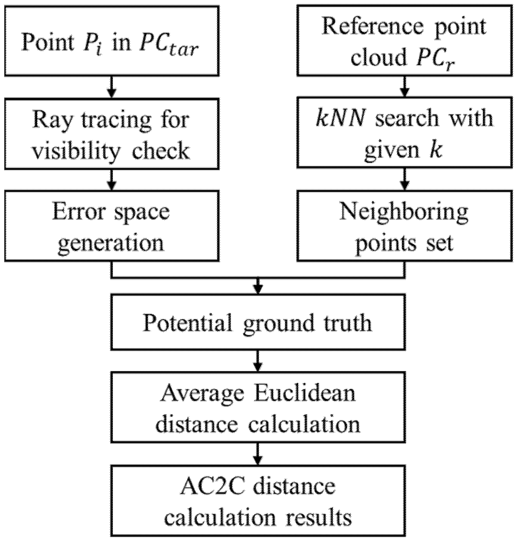
3. Proposed Methodology

The main ideas of the proposed methodology are (1) to use the point cloud with a higher theoretical accuracy and sufficient coverage as the $P{C}_{ref}$ to verify the $P{C}_{tar}$ generated from aerial photography; (2) to include the theoretical error of SfM-MVS to provide an adaptive “local region” for a neighboring points search. Although there are some differences between the processes of SfM and MVS, the dense point cloud generated by the expansion step in MVS follows the principle of “photometric discrepancy” [33]; therefore, the model adopted in the proposed method is theoretically applicable to both SfM and MVS. The proposed adaptive cloud-to-cloud (AC2C) comparison method is based on the C2C method but estimates the SfM-MVS measurement results more comprehensively. The significant steps of the proposed methodology are presented in Figure 2 and explained as follows:

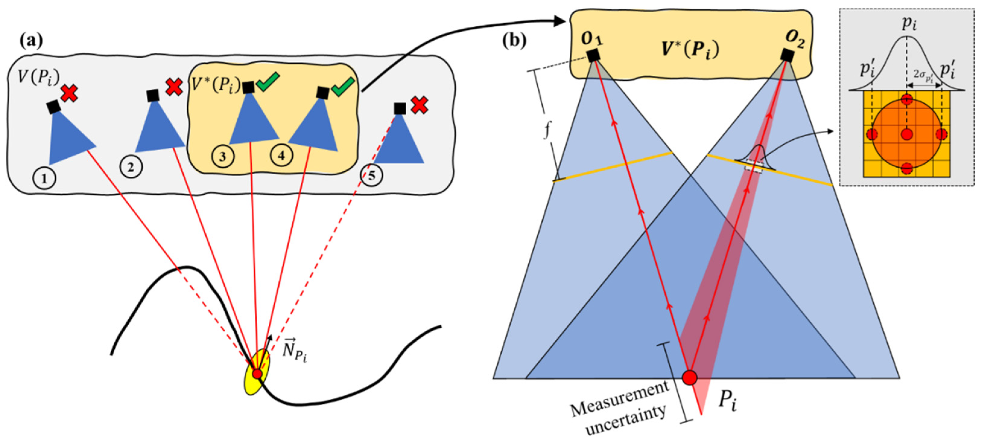
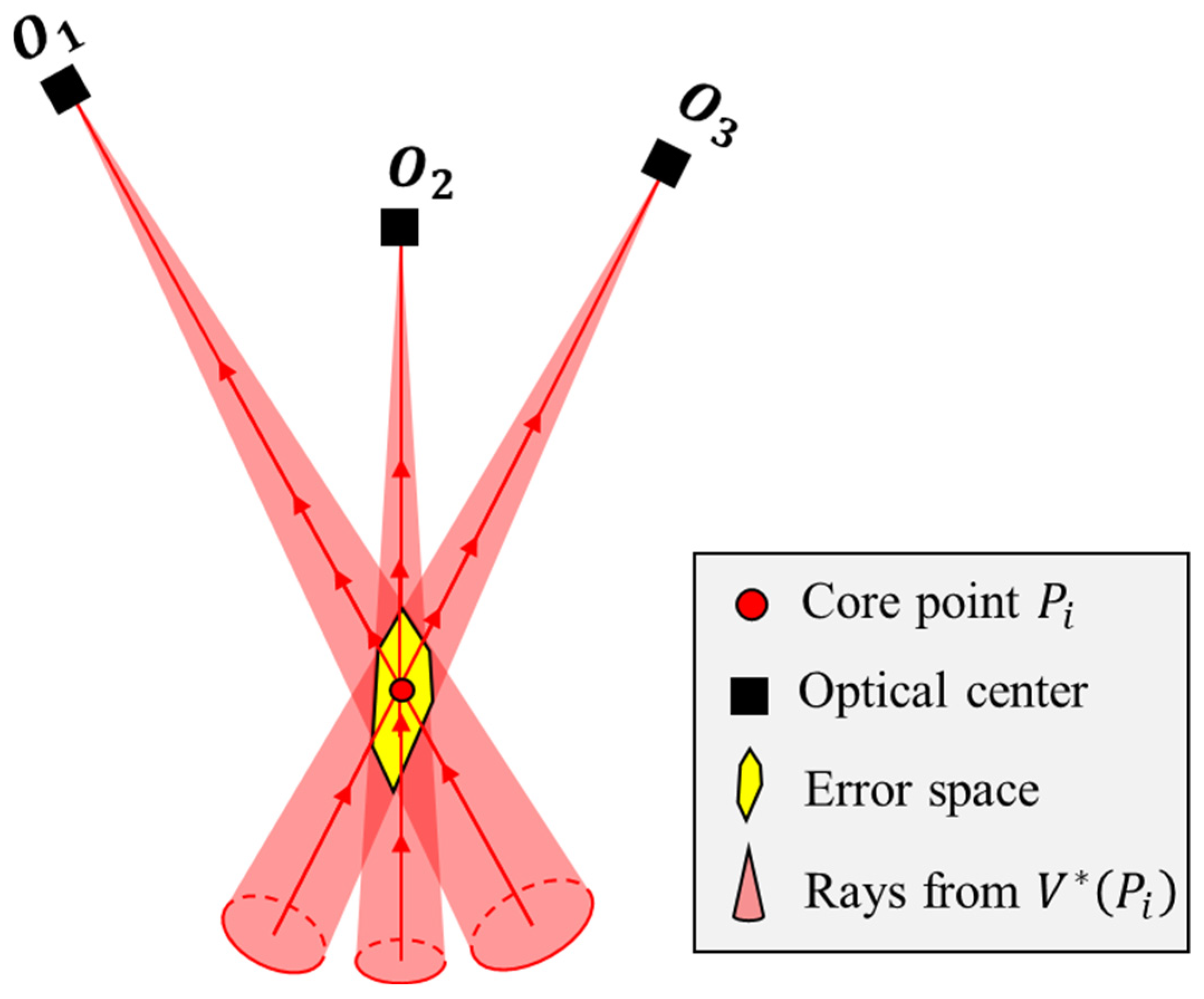
3.1. Step 1: Error Space Estimation

Before generating the error space for the target point $P_i$, a visibility check is essential to group the set of images $V\left(P_i\right)$ where $P_i$ is visible. Inspired by the calculation of the theoretical error model of MVS, the maximum angle between the viewing ray (a virtual light that connects the camera optical centers and $P_i$) and the local normal vector ${\overrightarrow{N}}_{P_i}$ is set as 30° to ensure image pairs in the $V\left(P_i\right)$ have an appropriate baseline. Then, the filtered $V\left(P_i\right)$ is represented as $V^{*}\left(P_i\right)$. Figure 3a illustrates five typical cameras in visibility checks marked as ①②③④⑤. Specifically, the viewing ray of camera ① is blocked by the $P{C}_{tar}$; the viewing ray of camera ② has an angle larger than 30° with ${\overrightarrow{N}}_{P_i}$; viewing rays in camera ③ and ④ satisfy the requirement; camera ⑤ shows a false positive viewing ray with no intersection with the sensor plane. It would be more rigorous but computationally expensive if all the photos were taken into account; therefore, to speed up the computation related to the subsequent error space estimations, the maximum angle between the viewing ray is set as 30°. Consequently, the image pairs where the maximum angle between the viewing rays is 60 degrees in $V^{*}\left(P_i\right)$ remains.

Figure 3b shows the measurement uncertainty of the stereo vision system. The error model is generally based on the BA introduced in the literature review section. For a typical convergent stereo vision system, $O_1$ and $O_2$ represent the optical center of two cameras with a focal length of $f$ and $P_i$ is the target point. Since the projection of $P_i$ on the sensor plane may have a certain degree of uncertainty, an inevitable difference exists between the position $p_i^{\prime }$, which results in a measurement error from the SfM-MVS. Assuming the position of $p_i^{\prime }$ around the actual projection position $p_i$ on the sensor plane following the Gaussian distribution:

$$g\left(p_i^{\prime }\right)=\exp \left[-\frac{1}{2}{\left(\frac{p_i^{\prime }-p_i}{{\sigma }_{p_i^{\prime }}}\right)}^2\right]$$

(5)

where ${\sigma }_{p_i^{\prime }}$ was suggested to be set as 2 pixels. The value of ${\sigma }_{p_i^{\prime }}$ can be adjusted according to the actual situation, but it needs to be at least larger than the value used in the reprojection error constraint, as explained in the literature review section.

It is challenging to compute the error space of multiple image pairs directly; therefore, the Boolean operation is adopted to approximate the error space in practice. Meanwhile, the convex envelope is applied to increase the robustness of the Boolean operation. Figure 4 displays the Boolean intersection output for three viewing rays, which are represented by the cones in red.

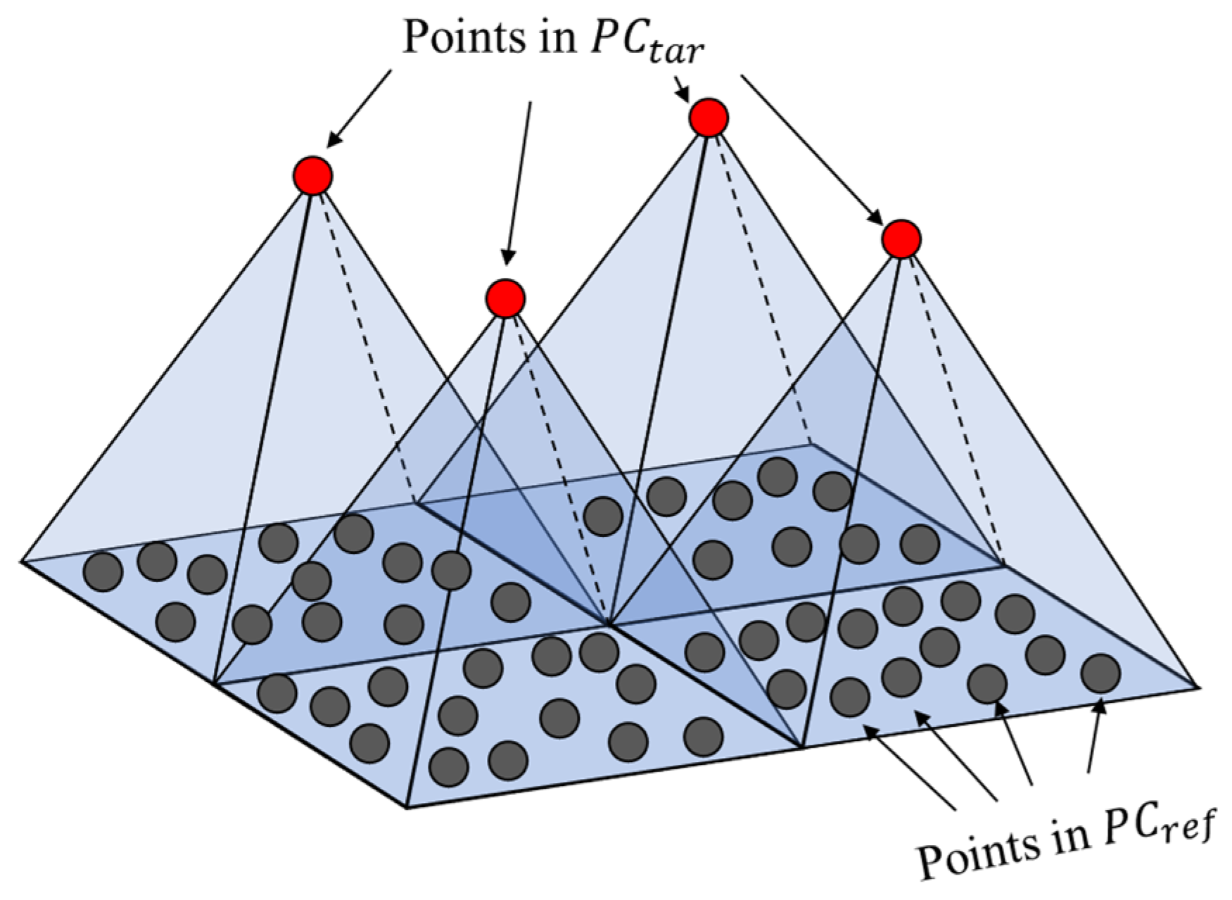
3.2. Step 2: Neighboring Points Search and Filtering

The error space generated from the previous step offers a promising lead for finding the “ground truth” of $P_i$ in the $P{C}_{ref}$; however, the space as the approximate output of the Boolean operation usually has a complex geometry and is difficult to be expressed in a concise mathematical expression. Therefore, directly searching out the points in the $P{C}_{ref}$ that are inside the error space can be expensive. As shown in Figure 5, to narrow down the searching range, a $k$-Nearest Neighbor (kNN) search is applied to find all candidates of $P_i$ in the $P{C}_{ref}$, shown as yellow dashed dots. Then, a filtering process is applied to filter those candidates $N_{r_{\sigma }}\left(P_i\right)$ within the boundary of the error space, shown as orange dots. Then, the filtered $N_{r_{\sigma }}\left(P_i\right)$ is represented as $N_{r_{\sigma }}^{*}\left(P_i\right)$.

Assuming the $P{C}_{ref}$ and $P{C}_{tar}$ are near uniformly distributed in a given area, the maximum number of neighbors that $k$ needs to consider depends on the ratio of density between the $P{C}_{ref}$ and $P{C}_{tar}$, as illustrated in Figure 6. The value of $k$ is recommended to be $\tau$ times the density ratio to provide enough buffer for those steep areas in the subsequent filtering processing ($\tau$ is suggested to be three or five according to our experiences). It is calculated according to Equation (6):

$$k=min\left\{n\in \mathbb{Z} | \left(\left|C_{ref}\right|/\left|C_{tar}\right|\right)\le n\right\}*\tau$$

(6)

where $\left|C_{ref}\right|$ and $\left|C_{tar}\right|$ are the number of points of the $P{C}_{ref}$ and $P{C}_{tar}$, respectively, and $\mathbb{Z}$ is the non-negative integer set. Note that the color information of the target point and the points in $N_{r_{\sigma }}\left(P_i\right)$ are not considered when implementing the kNN search since the color value of various photos taken by different sensors under different lighting conditions may be inconsistent.

3.3. Step 3: Measurement Error Evaluation

The kNN search and filtering in the previous step found all the potential corresponding “ground truths” for the $P_i$, which contributes to the error space. There are several methods to calculate the distance between these “ground truths” and $P_i$. For example, (1) following the C2M or C2C method introduced in the literature review section; (2) calculating the average distance from $P_i$ to all the points in $N_{r_{\sigma }}^{*}\left(P_i\right)$; (3) calculating the distance from $P_i$ to the average position of $N_{r_{\sigma }}^{*}\left(P_i\right)$ that was proposed by Lague et al. [28]. Since the point in both point clouds is not a dimensionless dot but a digital representation for a specific area with a particular physical size, all the points in $N_{r_{\sigma }}^{*}\left(P_i\right)$ should be taken into consideration. Additionally, since the error space is the output of the intersection of viewing rays, the weights of the distance ($d_{i,j}$) between $P_i$ and $N_{r_{\sigma }}^{*}\left(P_i\right)$ that contributed to the error space is assumed to follow the Gaussian function, which is calculated as Equation (7):

$$g_d\left(d_{i,j}\right)=\exp \left[-\frac{{\left(d_{i,j}-d_{min}\right)}^2}{2{\sigma }_d^2}\right]$$

(7)

where $d_{min}$ is the distance between $P_i$ and its nearest point in $N_{r_{\sigma }}^{*}\left(P_i\right)$. ${\sigma }_d$ has the same value with ${\sigma }_{GSD}$ according to the settings in Equation (5).

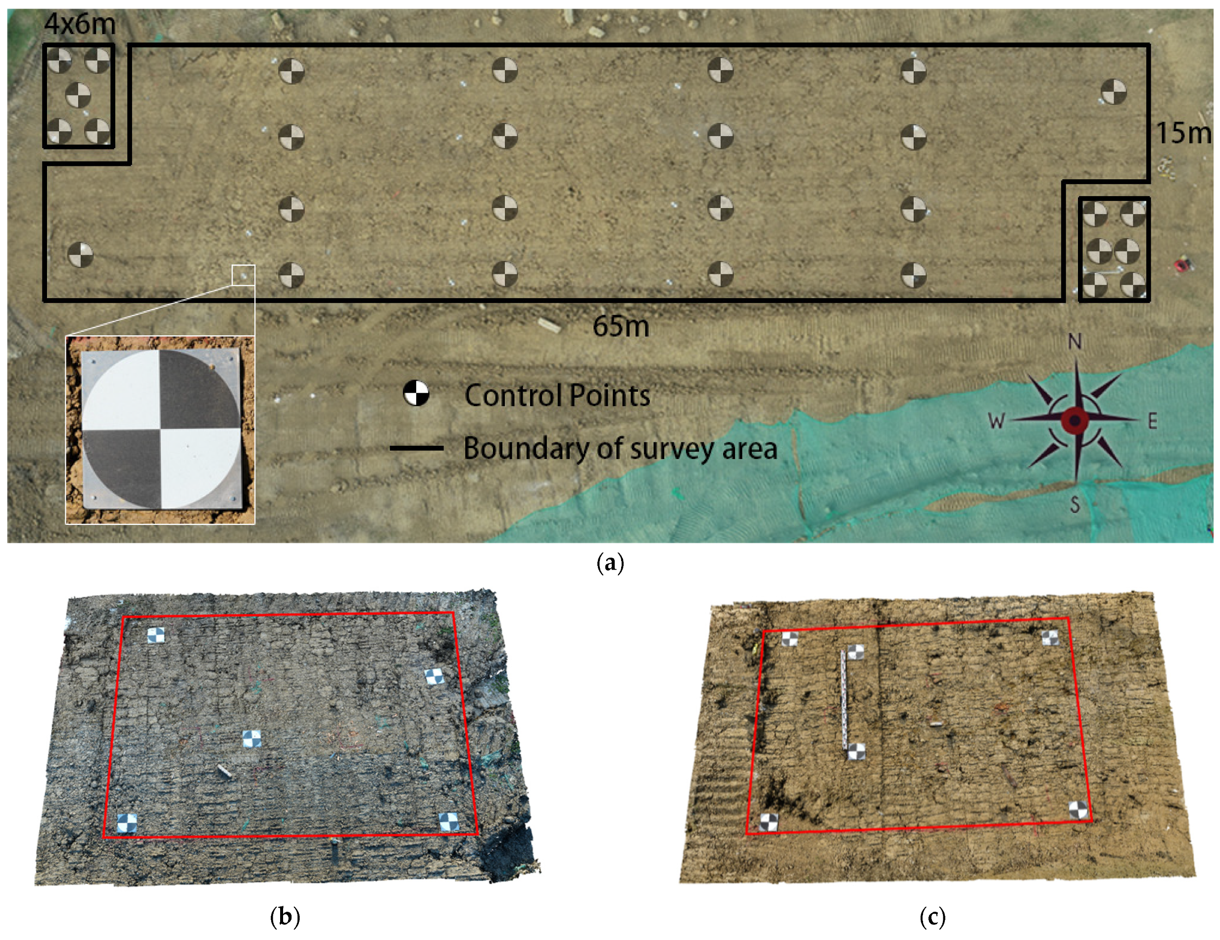
4. Data Collection and Setup

A field survey on bare soil was carried out to investigate the feasibility of the proposed methodology. Figure 7a shows that the experimental site was 15 m wide and 65 m long, with a height difference of 1.5 m. The topographic and geomorphic characteristics of the whole surveying and mapping area were relatively consistent, flat, and evenly covered by traces of excavator track. Two sub-areas (4 by 6 m) in each northwest corner (NWC) and southeast corner (SEC) were selected as the representative areas for an AC2C-based error estimation and placed with denser control points.

To provide a precise alignment between the $P{C}_{ref}$ and $P{C}_{tar}$, the targets that we used in this case study were specially designed, as shown in Figure 7a. Targets with a dimension of 30 × 30 × 0.3 cm were made using 6061 aluminum, a material with a relatively good stiffness and which is relatively lighter. An ultraviolet (UV) LED inkjet printer was used to print the black/white pattern on the surface of the targets. The printed surface has a high flatness, a sharp edge, and a distinct center point. Small holes were drilled at the four corners of the target with a diameter of 4.2 mm to fix on the bare soil with cement nails (a length of 64 mm and an outer diameter of 4 mm). When installing the targets, they were leveled by using a level bar. A total station (1 mm + 1 ppm, the standard deviation of the measurement was 1 mm, and the standard deviation increased 1 mm per kilometer away from the station) and a level (DS05, the standard deviation of the height difference of the per kilometer round trip was under 0.5 mm) were used to obtain the coordinates of the control points, and three local coordinate systems were established for UAV, NWC, and SEC surveying, respectively. The origin of the local coordinate system used for the UAV surveying was established on the south side of the study area, while the origins of the NWC and SEC were set on one of the scanning stations, respectively.

4.1. Data Collection for Reference Point Cloud

A commercial TLS, Leica ScanStation P40, with a ranging accuracy of 1.2 mm + 10 ppm and angular accuracy of ${\sigma }_{\tau }=8″$ was used in this case study. The scan rate (points/s) of the laser scanner was up to 1 million points per second, and the field of view was 360° in the horizontal and 270° in the vertical. More technical details are available in Walsh [46]. The laser scanner was mounted on a tripod about 1.6 m high. A total of four scans were used to fully cover each test field. The average registration error for the SEC and NWC was 1.52 mm and 1.21 mm. The average theoretical 3D coordinates measurement error in the surveying area was around 2.17 mm, according to the estimation method proposed by Huang et al. [47]. A more detailed description of the placement of the scan sites at the NWC and SEC and the density and accuracy of the laser point cloud within the test field can be found in the Supplementary Material.

4.2. Data Collection for Target Point Cloud

The aerial images were obtained using a DJI Phantom 4 RTK Unmanned Aerial Vehicle (UAV), specially designed for professional surveying and mapping. The resolution of the acquired images was 5472 × 3648 and the corresponding GSD at 25 m was 6.9 mm/px. Direct georeferencing was used. The on-board multi-frequency GNSS (Global Navigation Satellite System) receivers of the DJI Phantom 4 RTK are able to perform direct georeferencing in the workflow of SfM-MVS; however, in order to compare both point clouds in the following steps, they must be aligned to a common reference coordinate system. Therefore, control points (measured in the local coordinate system) were then applied for the point clouds registration between the ${\mathit{PC}}_{\mathit{tar}}$ and ${\mathit{PC}}_{\mathit{ref}}$. The built-in function of the UAV accomplished the flight path planning. The flight path adopted “five-way oblique photography” to achieve a high redundancy in the image collection. Each set of images would include one group of nadir photography and four groups of oblique photography from four different directions with the same oblique angle. The parameters for the flight path planning are shown in

Table 1. Parameters for flight path planning.

Fore-and-aft Overlap (%)	Side Overlap (%)	Height (m)	$\mathbf{Oblique} \mathbf{Angle} (°)$
90	90	25	10, 20, 30, 40, 45

. An amount of 300–500 photos were taken for each group, and the total number of photos taken by the UAV in the case study was about 1800.

As for the data collection, the images collected from the UAVs were calibrated with a calibration board. Then, the control points were installed, and their coordinates were measured using the total station. A commercial software, RealityCapture V1.2 was used to generate the $P{C}_{tar}$. The $P{C}_{tar}$ was computed in the high-quality mode to avoid the negative effect caused by the image resolution downscaling in the normal and preview modes. The maximal, median, and mean reprojection error (in pixel) of the bundle adjustment was 1.999, 0.5946, and 0.7052, respectively. Then, the alignment between the $P{C}_{tar}$ and $P{C}_{ref}$ was carried out via control points.

5. Results and Discussion

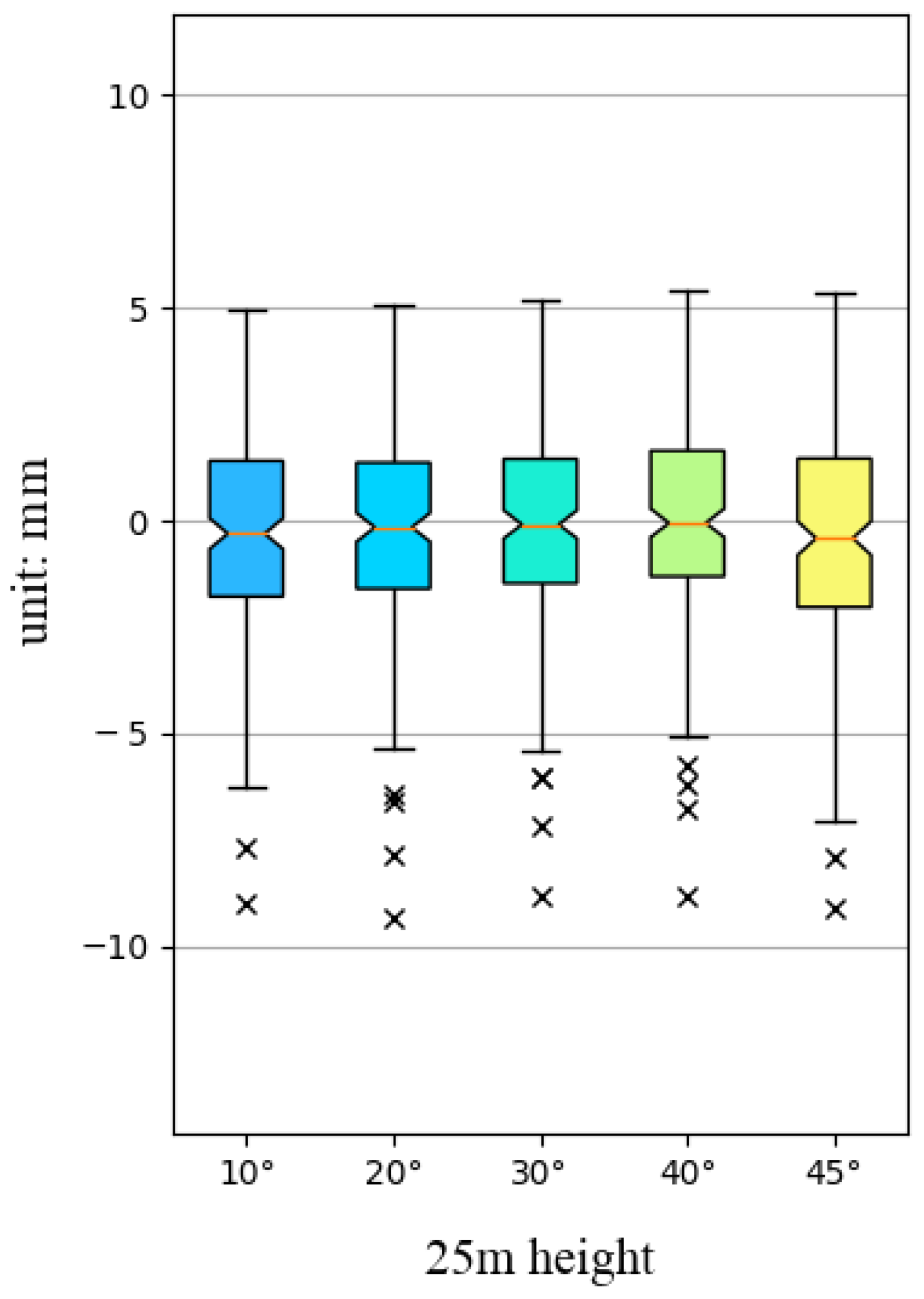
5.1. Measurement Error of Using Control Points

The coordinates of control points measured by the total station and level were taken as the reference values. The difference between the actual and calculated distances between any two control points was considered the measurement error. In total, 18 control points with 153 combinations were used to calculate the error, and the results are presented in Figure 8, where ‘x’ represents the outliers outside 1.5 times the interquartile range above the upper quartile and below the lower quartile. The mean values at different oblique angles were about 1.2 mm, which was smaller than the expected theoretical values (6.85 mm, 7.91 mm, and 3.95 mm) calculated by using Equation (1), Equation (2), and Equation (3), respectively; therefore, an “over-optimistic” evaluation of the accuracy of point clouds may occur in the case of using control points as a reference.

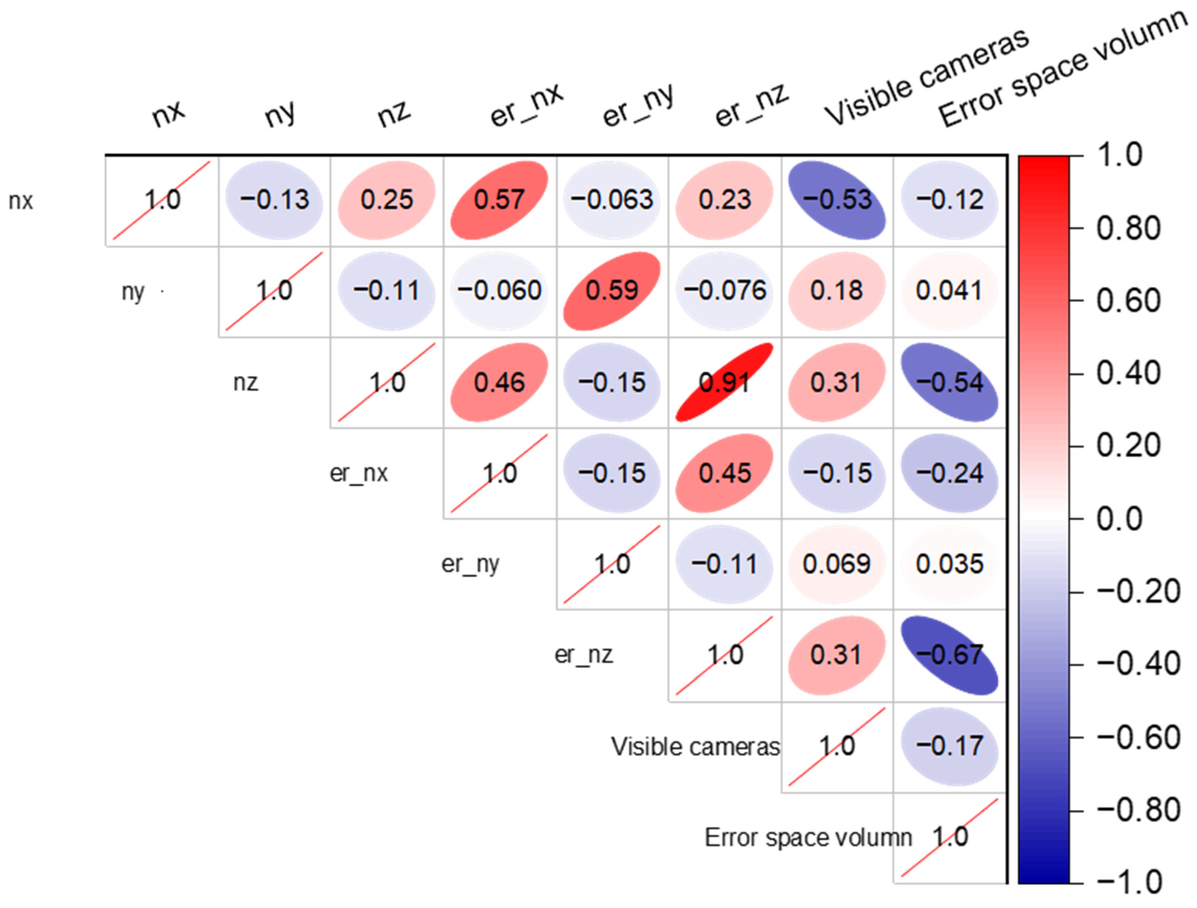
5.2. Visibility Check and Error Space Estimation

Figure 9 presents an example of the error space estimation and corresponding neighboring points searching and filtering in the SEC. Figure 9a shows the number of visible cameras at different locations in the SEC area. Normally, fewer cameras are visible in regions with a significant elevation variance since the viewing rays are likely to be occluded. Figure 9b shows the visible cameras in $V^{*}\left(P_i\right)$ for $P_i$, and the black sphere represents the camera optical center. The sensor planes are highlighted with the yellow rectangles, and the red lines represent the viewing ray leading from the camera center. In this case, $P_i$ was captured by 42 cameras. The angles between the local vector of $P_i$ and the viewing rays followed the requirement stated in the Methodology section; therefore, most of the image pairs in the $V^{*}\left(P_i\right)$ had an appropriate baseline to perform the triangulation. The Boolean intersection of the viewing rays is shown in grey in Figure 9d.

The $P{C}_{tar}$ contained about 182.2 thousand points and the $P{C}_{ref}$ contained about 26.3 million points. Consequently, the density ratio between the $P{C}_{ref}$ and $P{C}_{tar}$ was about 144:1; therefore, the k in the kNN search was set as 144 × 5 to provide enough candidate points before the filtering process. Figure 9c shows the result of the kNN search for $P_i$ in the $P{C}_{tar}$. The neighboring points are in blue, and $P_i$ is in red (for visualization purposes, the size of $P_i$ is enlarged).

Then, the approximate error space, the grey shape in Figure 9d, was used to identify the points inside the error space, resulting in the filtered points ($N_{r_{\sigma }}^{*}\left(P_i\right)$) in green, as shown in Figure 9e. The points in the set of $N_{r_{\sigma }}^{*}\left(P_i\right)$, as the intersection result of the error space and the $N_{r_{\sigma }}\left(P_i\right)$, preserve the characteristics of the error space, which has a particular direction; therefore, it provides a more reasonable “ground truth” as mentioned in the proposed methodology.

To further investigate the reliability of the estimated error spaces, a Pearson’s correlation coefficient matrix [48] was generated for the key parameters, as plotted in Figure 10. It was found that the orientation of the error space (er_nx, er_ny and er_nz) was strongly related to the local normal vector (nx, ny and nz), which indicates that the ray tracing for the visibility check was able to identify the corresponding cameras that can capture the $P_i$ correctly. Additionally, the volume of the error space negatively correlates to the total number of visible cameras. This means that the more visible cameras there are, the smaller the error space volume, which generally follows the basic principle of the theoretical error estimation of SfM-MVS stated in the methodology section. The results also verified the robustness of the error space estimation.

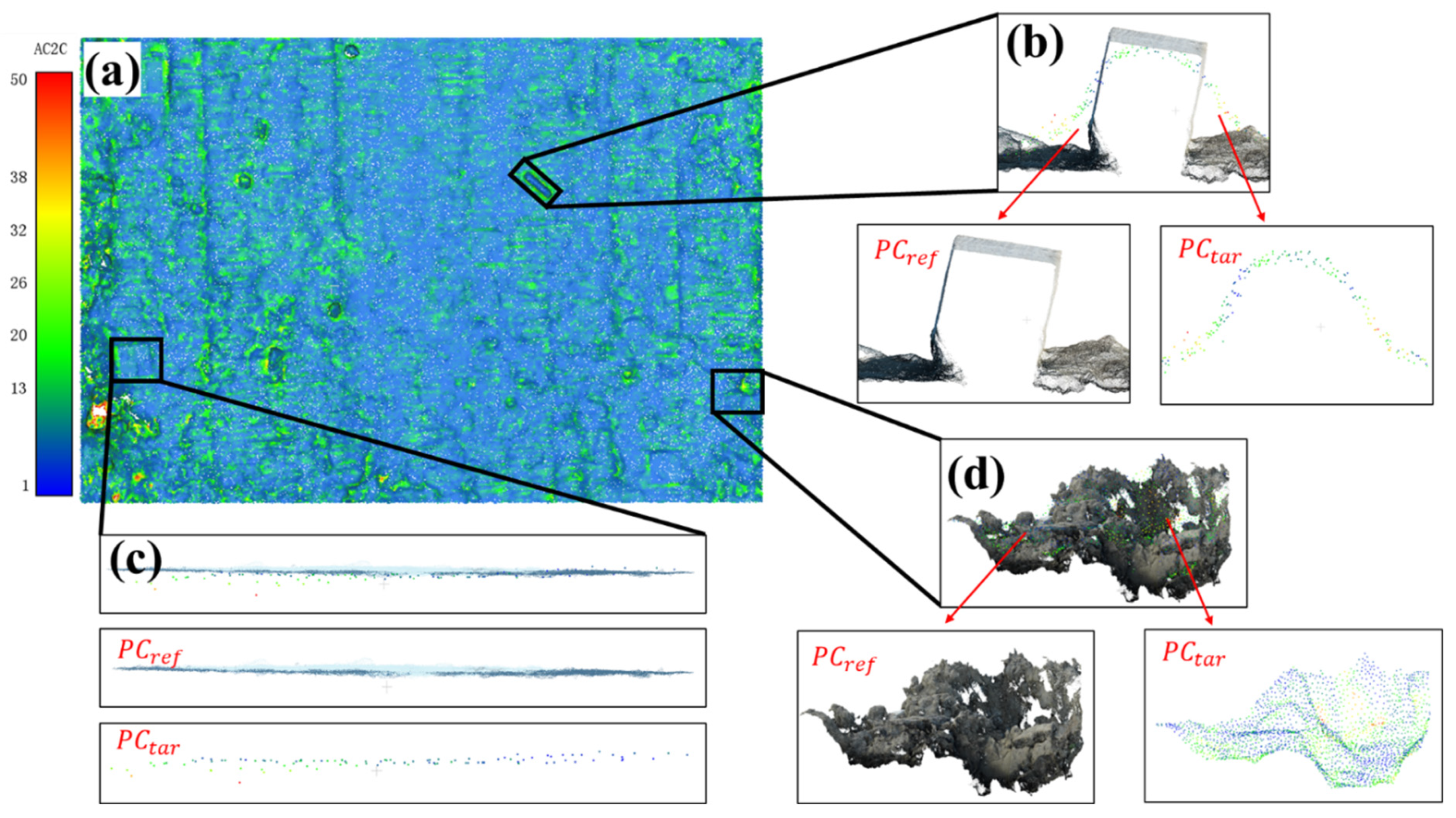
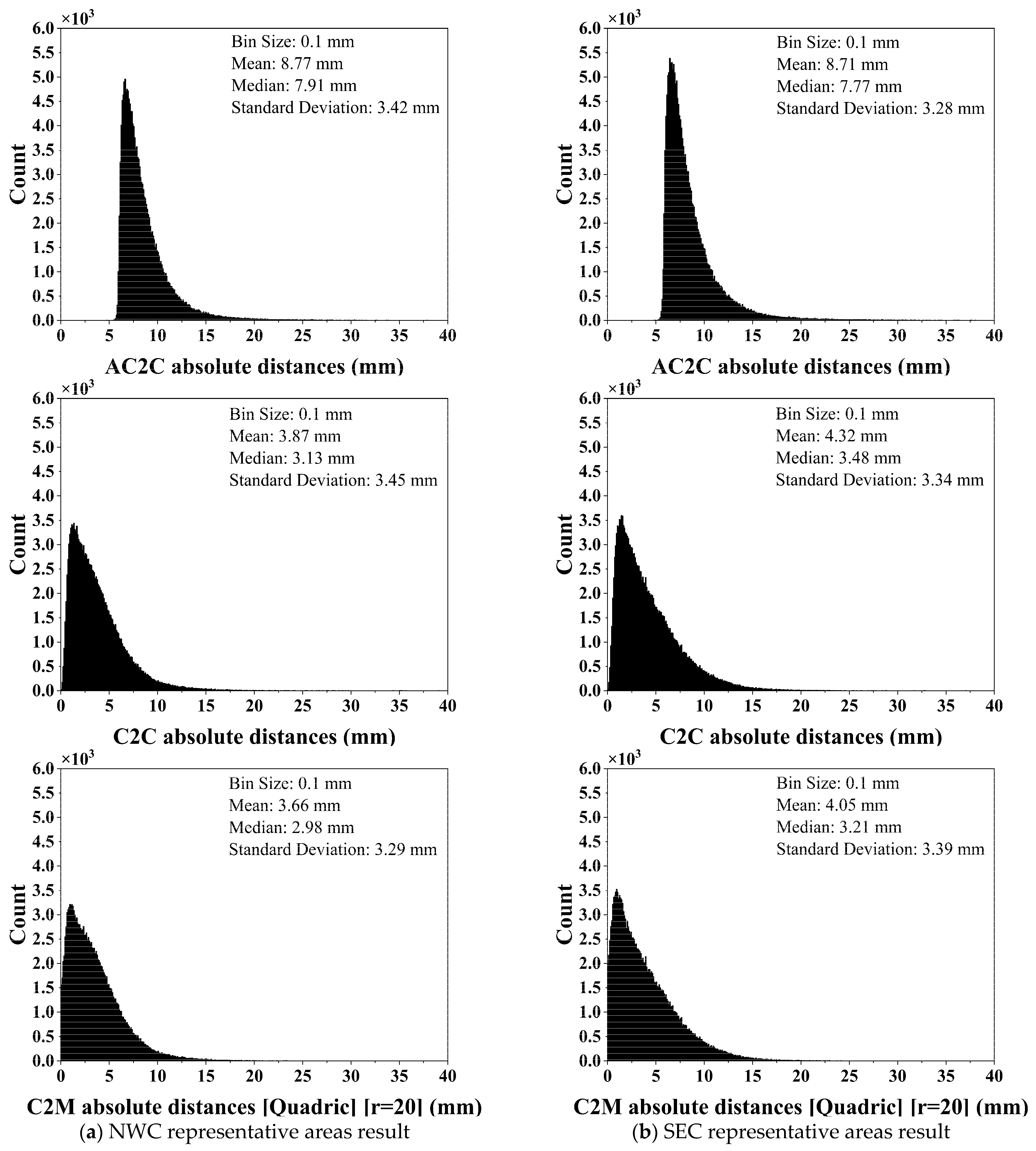
5.3. AC2C Distance Calculation Results

Based on the generated “ground truth”, the measurement error based on the AC2C method was calculated. For the aerial photography of the NWC, the flight height was set as 25 m, and the oblique angle was 30°. In Figure 11, the points in blue represent the minor errors, while the red ones represent the more significant ones. Figure 11a indicates that the overall error was low in the flat area, while significant errors frequently occurred on the surface with sharp changes in the normal vectors. For example, for a rectangle wood block placed on the surveying area, which is shown in Figure 11b, the points in the $P{C}_{ref}$ can basically represent its shape; however, the points in the $P{C}_{tar}$ failed to capture the sudden surface changes precisely since the edges of the reconstructed woodblock seemed to be smoothed off. For the aluminum target, which is shown in Figure 11c, the points from both the $P{C}_{tar}$ and $P{C}_{ref}$ were basically horizontally distributed and had small deviations in the vertical direction. The same situation occurred to those soil surfaces with acute changes. As shown in Figure 11d, for the potholes on the surface, the points in the $P{C}_{ref}$ were more accurate in presenting the depth and details of the potholes, but the points in the $P{C}_{tar}$ looked like a thin film covering the potholes, and all the shape and depth information was lost.

The largest differences often occur in the regions of steep faces (e.g., see lower right inset in Figure 12), due to the different acquisition and processing characteristics of the SfM-MVS and laser scanning. Missing data are found in the laser point cloud where a significant elevation variance occurs, since the TLS is susceptible to data gaps in locations not in the direct line-of-sight of the scanner, as shown in Figure 12. If the $P{C}_{ref}$ does not have sufficient distribution, the spatial variability of errors may remain unavailable.

Figure 13 presents the absolute distances calculation result of the AC2C and the two existing cloud comparison methods (C2C and C2M) for both the NWC area and SEC area. In the C2M method, the radius for the neighboring point search was set as 20 mm to provide enough neighboring points, and the local model was approximated with a quadric surface to fit the local change. In the figure, the bin size across all the histograms was set to a consistent width (0.1 mm) for visualization purposes.

As indicated in Figure 13, the absolute distances calculated from the three methods had basically the same range from 0 to 20 mm. The mean values (9.48 mm and 10.31 mm) of the AC2C were close to the GSD (6.9 mm), which was calculated in the section for the Data collection for target point cloud. The GSD is the index of the spatial resolution of the image, and it also reflects the approximate measurement error of the SfM-MVS; therefore, the result of the AC2C was reasonable, however, it can also be seen from the figure that the distribution of the AC2C results was more concentrated around 10 mm and rarely fell in the interval of 0–5 mm. This result matches the calculation mechanism introduced in Step 3 of the proposed methodology. Concretely, it first calculates all the distances from $P_i$ to the selected neighboring points $N_{r_{\sigma }}^{*}\left(P_i\right)$, and then takes the Gaussian weighted average distance as the measurement error, while the C2C and C2M usually return the closest distance to $N_{r_{\sigma }}^{*}\left(P_i\right)$; therefore, in most cases, the C2C and C2M result in a much smaller value than that of the AC2C that includes all the points within $N_{r_{\sigma }}^{*}\left(P_i\right)$.

6. Conclusions

The present paper proposes an AC2C comparison method for photogrammetry point cloud error estimation considering the theoretical error space. Compared to the existing techniques, the AC2C method introduces new elements (e.g., ray tracing, visibility check, and error space generation) according to the theoretical error of SfM-MVS to provide a more reliable “ground truth” in the $P{C}_{ref}$ for the $P{C}_{tar}$. Additionally, the calculation of the distance between $P_i$ and $N_{r_{\sigma }}^{*}\left(P_i\right)$ is improved by using the weighted average distance (according to the probability distribution inside the error space) rather than directly taking the distance to the average position of $N_{r_{\sigma }}^{*}\left(P_i\right)$ or the distance to the closest neighboring point.

A field survey was carried out to demonstrate the feasibility of the proposed method. The analysis result from the correlation coefficient matrix indicates that the property of the error space (e.g., major direction and volume) is consistent with the principle of triangulation in SfM-MVS; thus, the error space estimated according to the proposed method is reliable and useful in selecting the potential “ground truth” from the neighboring points in the $P{C}_{ref}$. Additionally, compared to the results calculated from the C2C and C2M methods, the results of the AC2C method have a larger mean value due to its unique definition in the distance calculation between these “ground truths”. This mean value is closer to the theoretical value and is more consistent with the actual situation; therefore, the proposed method is more objective and reliable in evaluating the measurement error of photogrammetry-based 3D reconstruction in practice. It improves the existing distance measurement solutions by introducing a link between the working principle of SfM-MVS and error evaluation methods.

However, accurately evaluating the error of SfM-MVS is still challenging due to the existence of the error in the GCP center localization and point clouds registration. The AC2C works fully in 3D, costing more calculation time than the C2C and C2M methods, especially in an error space estimation. Compared with AC2C, the C2C comparison method does not require gridding or meshing of the data, nor a calculation of the surface normal, which has a lower computational load; however, the cloud-to-cloud (C2C) and cloud-to-mesh (C2M) comparison methods usually consider either the closest point or the neighboring points within a fixed searching radius as the “ground truth”, which may not reflect the actual accuracy. The error space in the AC2C is estimated according to the position of the corresponding visible cameras and their distances to the target point, which can return a reliable potential “ground truth”.

In the future, the computing efficiency of AC2C should be improved, and its feasibility should be verified in a more demanding field test which should include objects with a significant elevation difference of about a few meters. Additionally, instead of using several local coordinate systems, a consistent coordinate system should be applied to provide a more comprehensive accuracy analysis.

References

1. Moon, D.; Chung, S.; Kwon, S.; Seo, J.; Shin, J. Comparison and utilization of point cloud generated from photogrammetry and laser scanning: 3D world model for smart heavy equipment planning. Autom. Constr. 2019, 98, 322–331. [Google Scholar] [CrossRef]
2. Saovana, N.; Yabuki, N.; Fukuda, T. Development of an unwanted-feature removal system for Structure from Motion of repetitive infrastructure piers using deep learning. Adv. Eng. Inform. 2020, 46, 101169. [Google Scholar] [CrossRef]
3. Balali, V.; Jahangiri, A.; Machiani, S.G. Multi-class US traffic signs 3D recognition and localization via image-based point cloud model using color candidate extraction and texture-based recognition. Adv. Eng. Inform. 2017, 32, 263–274. [Google Scholar] [CrossRef]
4. Lane, S.N.; James, T.D.; Crowell, M.D. Application of Digital Photogrammetry to Complex Topography for Geomorphological Research. Photogramm. Rec. 2000, 16, 793–821. [Google Scholar] [CrossRef]
5. Chio, S.-H.; Chiang, C.-C. Feasibility Study Using UAV Aerial Photogrammetry for a Boundary Verification Survey of a Digitalized Cadastral Area in an Urban City of Taiwan. Remote Sens. 2020, 12, 1682. [Google Scholar] [CrossRef]
6. Grenzdörffer, G.; Engel, A.; Teichert, B. The photogrammetric potential of low-cost UAVs in forestry and agriculture. Int. Arch. Photogramm. Remote Sens. Spat. Inf. Sci. 2008, 31, 1207–1214. [Google Scholar]
7. Lo, Y.; Zhang, C.; Ye, Z.; Cui, C. Monitoring road base course construction progress by photogrammetry-based 3D reconstruction. Int. J. Constr. Manag. 2022, 1–15. [Google Scholar] [CrossRef]
8. Shi, Z.; Lin, Y.; Li, H. Extraction of urban power lines and potential hazard analysis from mobile laser scanning point clouds. Int. J. Remote Sens. 2020, 41, 3411–3428. [Google Scholar] [CrossRef]
9. Gao, L.; Zhang, X. Above-Ground Biomass Estimation of Plantation with Complex Forest Stand Structure Using Multiple Features from Airborne Laser Scanning Point Cloud Data. Forests 2021, 12, 1713. [Google Scholar] [CrossRef]
10. Balsa-Barreiro, J.; Fritsch, D. Generation of visually aesthetic and detailed 3D models of historical cities by using laser scanning and digital photogrammetry. Digit. Appl. Archaeol. Cult. Herit. 2018, 8, 57–64. [Google Scholar] [CrossRef]
11. Wallace, L.; Lucieer, A.; Malenovský, Z.; Turner, D.; Vopěnka, P. Assessment of Forest Structure Using Two UAV Techniques: A Comparison of Airborne Laser Scanning and Structure from Motion (SfM) Point Clouds. Forests 2016, 7, 62. [Google Scholar] [CrossRef] [Green Version]
12. White, J.C.; Wulder, M.A.; Vastaranta, M.; Coops, N.C.; Pitt, D.; Woods, M. The Utility of Image-Based Point Clouds for Forest Inventory: A Comparison with Airborne Laser Scanning. Forests 2013, 4, 518–536. [Google Scholar] [CrossRef]
13. Green, S.; Bevan, A.; Shapland, M. A comparative assessment of structure from motion methods for archaeological research. J. Archaeol. Sci. 2014, 46, 173–181. [Google Scholar] [CrossRef]
14. James, M.R.; Robson, S. Straightforward reconstruction of 3D surfaces and topography with a camera: Accuracy and geoscience application. J. Geophys. Res.-Earth Surf. 2012, 117, 17. [Google Scholar] [CrossRef]
15. Barazzetti, L. Network design in close-range photogrammetry with short baseline images. In Proceedings of the 26th International CIPA Symposium on Digital Workflows for Heritage Conservation, Ottawa, ON, Canada, 28 August–1 September 2017; pp. 17–23. [Google Scholar]
16. Luhmann, T.; Fraser, C.; Maas, H.G. Sensor modelling and camera calibration for close-range photogrammetry. Isprs J. Photogramm. Remote Sens. 2016, 115, 37–46. [Google Scholar] [CrossRef]
17. Sapirstein, P. Accurate measurement with photogrammetry at large sites. J. Archaeol. Sci. 2016, 66, 137–145. [Google Scholar] [CrossRef]
18. Tavani, S.; Pignalosa, A.; Corradetti, A.; Mercuri, M.; Smeraglia, L.; Riccardi, U.; Seers, T.; Pavlis, T.; Billi, A. Photogrammetric 3D Model via Smartphone GNSS Sensor: Workflow, Error Estimate, and Best Practices. Remote Sens. 2020, 12, 3616. [Google Scholar] [CrossRef]
19. Eltner, A.; Kaiser, A.; Castillo, C.; Rock, G.; Neugirg, F.; Abellán, A. Image-based surface reconstruction in geomorphometry—Merits, limits and developments. Earth Surf. Dyn. 2016, 4, 359–389. [Google Scholar] [CrossRef]
20. James, M.R.; Robson, S.; Smith, M.W. 3-D uncertainty-based topographic change detection with structure-from-motion photogrammetry: Precision maps for ground control and directly georeferenced surveys. Earth Surf. Processes Landf. 2017, 42, 1769–1788. [Google Scholar] [CrossRef]
21. Harwin, S.; Lucieer, A. Assessing the Accuracy of Georeferenced Point Clouds Produced via Multi-View Stereopsis from Unmanned Aerial Vehicle (UAV) Imagery. Remote Sens. 2012, 4, 1573–1599. [Google Scholar] [CrossRef]
22. Martinez-Carricondo, P.; Aguera-Vega, F.; Carvajal-Ramirez, F.; Mesas-Carrascosa, F.J.; Garcia-Ferrer, A.; Perez-Porras, F.J. Assessment of UAV-photogrammetric mapping accuracy based on variation of ground control points. Int. J. Appl. Earth Obs. Geoinf. 2018, 72, 1–10. [Google Scholar] [CrossRef]
23. Tonkin, T.N.; Midgley, N.G. Ground-Control Networks for Image Based Surface Reconstruction: An Investigation of Optimum Survey Designs Using UAV Derived Imagery and Structure-from-Motion Photogrammetry. Remote Sens. 2016, 8, 786. [Google Scholar] [CrossRef]
24. Luhmann, T. 3D Imaging—How to Achieve Highest Accuracy. In Proceedings of the Conference on Videometrics, Range Imaging, and Applications XI, Munich, Germany, 25–26 May 2011. [Google Scholar]
25. Luhmann, T. Close range photogrammetry for industrial applications. Isprs J. Photogramm. Remote Sens. 2010, 65, 558–569. [Google Scholar] [CrossRef]
26. Huang, H.; Ye, Z.; Zhang, C. An Innovative Approach of Evaluating the Accuracy of Point Cloud Generated by Photogrammetry-Based 3D Reconstruction. In Computing in Civil Engineering, Proceedings of the ASCE International Conference on Computing in Civil Engineering, Orlando, FL, USA, 12–14 September 2021; ASCE: Reston, VA, USA, 2021; pp. 926–933. [Google Scholar]
27. Gómez-Gutiérrez, Á.; Sanjosé-Blasco, D.; Juan, J.; Lozano-Parra, J.; Berenguer-Sempere, F.; Matías-Bejarano, D. Does HDR pre-processing improve the accuracy of 3D models obtained by means of two conventional SfM-MVS software packages? The case of the Corral del Veleta rock glacier. Remote Sens. 2015, 7, 10269–10294. [Google Scholar] [CrossRef]
28. Lague, D.; Brodu, N.; Leroux, J. Accurate 3D comparison of complex topography with terrestrial laser scanner: Application to the Rangitikei canyon (N-Z). ISPRS J. Photogramm. Remote Sens. 2013, 82, 10–26. [Google Scholar] [CrossRef]
29. Triggs, B.; McLauchlan, P.F.; Hartley, R.I.; Fitzgibbon, A.W. Bundle adjustment—A modern synthesis. In Proceedings of the International Workshop on Vision Algorithms, Corfu, Greece, 21–22 September 1999; pp. 298–372. [Google Scholar]
30. Szeliski, R. Computer Vision: Algorithms and Applications; Springer Science & Business Media: Berlin/Heidelberg, Germany, 2010. [Google Scholar]
31. Smith, M.W.; Carrivick, J.L.; Quincey, D.J. Structure from motion photogrammetry in physical geography. Prog. Phys. Geogr. 2016, 40, 247–275. [Google Scholar] [CrossRef]
32. Ahmadabadian, A.H.; Robson, S.; Boehm, J.; Shortis, M.; Wenzel, K.; Fritsch, D. A comparison of dense matching algorithms for scaled surface reconstruction using stereo camera rigs. ISPRS J. Photogramm. Remote Sens. 2013, 78, 157–167. [Google Scholar] [CrossRef]
33. Furukawa, Y.; Ponce, J. Accurate, Dense, and Robust Multiview Stereopsis. IEEE Trans. Pattern Anal. Mach. Intell. 2010, 32, 1362–1376. [Google Scholar] [CrossRef]
34. Furukawa, Y.; Curless, B.; Seitz, S.M.; Szeliski, R. Towards Internet-scale multi-view stereo. In Proceedings of the 2010 IEEE Computer Society Conference on Computer Vision and Pattern Recognition, San Francisco, CA, USA, 13–18 June 2010; pp. 1434–1441. [Google Scholar]
35. Nesbit, P.R.; Hugenholtz, C.H. Enhancing UAV-SfM 3D Model Accuracy in High-Relief Landscapes by Incorporating Oblique Images. Remote Sens. 2019, 11, 239. [Google Scholar] [CrossRef]
36. James, M.R.; Antoniazza, G.; Robson, S.; Lane, S.N. Mitigating systematic error in topographic models for geomorphic change detection: Accuracy, precision and considerations beyond off-nadir imagery. Earth Surf. Processes Landf. 2020, 45, 2251–2271. [Google Scholar] [CrossRef]
37. Felipe-García, B.; Hernández-López, D.; Lerma, J.L. Analysis of the ground sample distance on large photogrammetric surveys. Appl. Geomat. 2012, 4, 231–244. [Google Scholar] [CrossRef]
38. Nagendran, S.K.; Tung, W.Y.; Ismail, M.A.M. Accuracy assessment on low altitude UAV-borne photogrammetry outputs influenced by ground control point at different altitude. In IOP Conference Series: Earth and Environmental Science, Proceedings of the 9th IGRSM International Conference and Exhibition on Geospatial & Remote Sensing (IGRSM 2018), Kuala Lumpur, Malaysia, 24–25 April 2018; IOP Publishing: Bristol, UK, 2018; p. 012031. [Google Scholar]
39. Girardeau-Montaut, D.; Roux, M.; Marc, R.; Thibault, G. Change detection on points cloud data acquired with a ground laser scanner. Int. Arch. Photogramm. Remote Sens. Spat. Inf. Sci. 2005, 36, W19. [Google Scholar]
40. Jafari, B.; Khaloo, A.; Lattanzi, D. Deformation Tracking in 3D Point Clouds Via Statistical Sampling of Direct Cloud-to-Cloud Distances. J. Nondestruct. Eval. 2017, 36, 10. [Google Scholar] [CrossRef]
41. Carrea, D.; Abellan, A.; Derron, M.H.; Jaboyedoff, M. Automatic Rockfalls Volume Estimation Based on Terrestrial Laser Scanning Data. In Proceedings of the 12th International IAEG Congress, Torino, Italy, 15–19 September 2014; pp. 425–428. [Google Scholar]
42. Cignoni, P.; Rocchini, C.; Scopigno, R. Metro: Measuring error on simplified surfaces. Comput. Graph. Forum 1998, 17, 167–174. [Google Scholar] [CrossRef]
43. Charbonnier, P.; Chavant, P.; Foucher, P.; Muzet, V.; Prybyla, D.; Perrin, T.; Grussenmeyer, P.; Guillemin, S. Accuracy assessment of a canal-tunnel 3d model by comparing photogrammetry and laserscanning recording techniques. ISPRS-Int. Arch. Photogramm. Remote Sens. Spat. Inf. Sci. 2013, XL-5/W2, 171–176. [Google Scholar] [CrossRef]
44. Favalli, M.; Fornaciai, A.; Isola, I.; Tarquini, S.; Nannipieri, L. Multiview 3D reconstruction in geosciences. Comput. Geosci. 2012, 44, 168–176. [Google Scholar] [CrossRef]
45. DiFrancesco, P.M.; Bonneau, D.; Hutchinson, D.J. The Implications of M3C2 Projection Diameter on 3D Semi-Automated Rockfall Extraction from Sequential Terrestrial Laser Scanning Point Clouds. Remote Sens. 2020, 12, 1885. [Google Scholar] [CrossRef]
46. Walsh, G. Leica scanstation P-series—Details that matter. In Leica ScanStation—White Paper; Leica Geosystems AG: St. Gallen, Switzerland, 2015. [Google Scholar]
47. Huang, H.; Zhang, C.; Hammad, A. Effective Scanning Range Estimation for Using TLS in Construction Projects. J. Constr. Eng. Manage. 2021, 147, 13. [Google Scholar] [CrossRef]
48. Pearson, K.; Galton, F., VII. Note on regression and inheritance in the case of two parents. Proc. R. Soc. Lond. 1895, 58, 240–242. [Google Scholar] [CrossRef]
Figure 1. Gaussian weight to the angle (adopted from Furukawa et al. [34]).
Remotesensing 14 04289 g001
Figure 2. Major steps of the AC2C comparison method.
Remotesensing 14 04289 g002
Figure 3. Error space generation. (a) Visibility check; (b) measurement uncertainty.
Remotesensing 14 04289 g003
Figure 4. Boolean operation and error space.
Remotesensing 14 04289 g004
Figure 5. Neighboring point search and filtering.
Remotesensing 14 04289 g005
Figure 6. Relationship between the density of P C r e f and P C t a r .
Remotesensing 14 04289 g006
Figure 7. Overview of the experimental site and two representative areas on the corners. (a) Overview of the whole experimental site; (b) northwest corner (NWC); (c) southeast corner (SEC).
Remotesensing 14 04289 g007
Figure 8. Distribution of measurement errors at different oblique angles.
Remotesensing 14 04289 g008
Figure 9. Error space estimation and neighboring points searching and filtering. (a) Distribution of number of visible cameras; (b) ray tracing for visibility check; (c) kNN search result; (d) intersection with error space; (e) filtered neighboring points.
Remotesensing 14 04289 g009
Figure 10. Pearson correlation coefficient matrix of key parameters.
Remotesensing 14 04289 g010
Figure 11. AC2C distance calculation results and details in NWC. (a) overview, (b) wood block, (c) control point, and (d) potholes on the surface.
Remotesensing 14 04289 g011
Figure 12. Missing data due to occlusion. (a) overview of laser point cloud and (b) area with significant missing data.
Remotesensing 14 04289 g012
Figure 13. Absolute distances calculation result for (a) NWC and (b) SEC.
Remotesensing 14 04289 g013