Abstract
Accurate and up-to-date land cover classification information is essential for many applications, such as land-use change detection, global environmental change, and forest management, among others. Unoccupied aerial systems (UASs) provide the advantage of flexible and rapid data acquisition at low cost compared to conventional platforms, such as satellite and airborne systems. UASs are often equipped with high spatial resolution cameras and/or light detection and ranging (LiDAR). However, the high spatial resolution imagery has a high information content, which makes land cover classification quite challenging. Recently, deep convolutional neural networks (DCNNs) have been effectively applied to remote sensing applications, which overcome the drawback of traditional techniques. In this research, a low-cost UAV-based multi-sensor data fusion model was developed for land cover classification based on a DCNN. For the purpose of this research, two datasets were collected at two different urban locations using two different UASs. A DCNN model, based on U-net with Resnet101 as a backbone, was used to train and test the fused image/LiDAR data. The maximum likelihood and support vector machine techniques were used as a reference for classifier comparison. It was shown that the proposed DCNN approach improved the overall accuracy of land cover classification for the first dataset by 15% compared to the reference classifiers. In addition, the overall accuracy of land cover classification improved by 7%, and the precision, recall, and F-measure improved by 18% when the fused image/LiDAR data were used compared to the images only. The trained DCNN model was also tested on the second dataset, and the obtained results were largely similar to those of the first dataset.
1. Introduction
Land cover classification is a critical task in many applications, such as land management and planning, disaster monitoring, and climate change [1,2]. Recently, the use of small unoccupied aerial systems (UASs) in remote sensing applications has been extensively investigated [3,4,5,6]. UASs can potentially provide high spatial and temporal resolution data at low cost compared to conventional airborne systems. In addition, recent development in sensor technology has increased the payload capabilities of UAVs to include multiple sensors, such as high spatial resolution cameras, multispectral cameras, and light detection and ranging (LiDAR). For example, Lv et al. [7] used UAV-based RGB images to classify seven land cover classes including buildings, grass, road, trees, water, soil, and shadows. Their proposed approach object filter based on topology and features (OFTF) achieved an overall accuracy of 94% and a kappa coefficient of 92%. Natesan et al. [8] equipped a rotary-wing UAV with RGB and NIR cameras to image riverine areas for classifying four classes, achieving a 78% accuracy. In [9], the authors utilized UAV-based multispectral images for land-cover classification in a mining area. The multispectral images were composed of four bands, namely, red, green, blue, and near-infrared. They were used for training and testing seven U-Net models to classify six land cover types, and they achieved an accuracy of 83.6%. In [10], a UAV equipped with a four-band multi-spectral camera was used to classify four land cover classes. Three classification techniques were compared, namely, pixel-based, boosting-based, and object-based random forest (RF-O). Their results showed that the RF-O approach achieved the highest classification accuracy of 92%, and the kappa coefficient was 89%. In [11], a fixed-wing aircraft equipped with various sensors including RGB, thermal infrared, and 5-band multi-spectral sensors was used to create land cover maps. A total of nine orthoimages were produced and classified using the random forest (RF) classifier. The kappa coefficient was 72% with an overall accuracy of 76%.
Very high-resolution images provide a high level of detail, which makes them a good source of high horizontal-accuracy data with rich spectral and textural information crucial for segmentation and classification [12,13]. However, one of the limitations of these passive sensors is neglecting the vertical dimension of the ground features due to their inability to collect three-dimensional (3D) data [14]. Consequently, the accuracy of land cover classification is reduced because images are not suitable for differentiating classes that have similar spectral characteristics, such as building rooftops and roads. On the other hand, LiDAR can acquire 3D point clouds, providing accurate vertical information. However, low-cost LiDAR systems have limited spectral information. Previous studies have shown that the fusion of LiDAR data and images can provide complementary information, which improves the accuracy of land cover classification [15,16,17,18]. For example, Reese et al. [15] fused airborne LiDAR and satellite image data to classify alpine vegetation, which resulted in higher classification accuracy. In [19], a new approach was developed to fuse LiDAR data and a QuickBird image, which improved the overall accuracy by approximately 14% compared to the image data only. Bork and Su [20] showed that integrating LiDAR data and multispectral imagery increased the vegetation classification accuracy by 16 to 20%. In [21], LiDAR intensity was integrated with airborne multispectral camera images to classify eight agricultural land uses. Their results showed that the overall classification accuracy was improved by up to 40% compared with that obtained using the multispectral images only.
Many methods of land cover classification using high spatial resolution data have been proposed. Generally, the classification methods can be divided into pixel-based and object-based approaches [22]. The former approach identifies classes for individual pixels based on their spectral characteristics. In very high-resolution imagery, the spatial context from surrounding pixels is not considered in the classification process of pixel-based methods, which may cause a salt and pepper effect [23]. Therefore, object-based approaches were introduced to solve this problem, where neighboring pixels are merged into objects using segmentation techniques [24]. However, the classification accuracy is significantly affected by the segmentation quality [25,26]. In addition, a specific set of object features and parameters needs to be selected arbitrarily at the beginning, which affects the effectiveness and the accuracy of the classification process [27]. Furthermore, in complex urban areas, the selected features may not be representative of all land cover classes [24]. Therefore, an automatic feature learning approach from remote sensing data is needed.
Recently, deep convolutional neural networks (DCNNs) have achieved remarkable results in image classification and segmentation for remote sensing applications. For example, DCNN semantic segmentation methods have shown great potential in land cover classification [28,29,30,31]. In [28], a DCNN approach was proposed for land use classification in two areas using multispectral images. Their proposed approach obtained an overall accuracy of 91% and a kappa coefficient of 90% for the first area and an overall accuracy of 80% and a kappa coefficient of 78% for the second area. In [30], two DCNNs were compared, namely, the Sharpmask model [32] and the RefineNet model [33]. Both networks were trained and tested on a dataset created by the authors called RIT-18. The RIT-18 dataset was collected using a UAV equipped with multiple sensors. The dataset consisted of six spectral bands and eighteen labelled object classes. The Sharpmask model obtained a mean-class accuracy of approximately 57%, while the RefineNet model obtained a mean-class accuracy of approximately 59%. The U-net model proposed by Ronneberger et al. [34] is an updated fully convolutional network (FCN) model with a symmetrical U-shape divided into two main components, namely, an encoder and a decoder. The encoder part is used for extracting features, while the decoder is used for upsampling operations. It integrates low-level features with detailed spatial information to boost segmentation accuracy [35]. The U-net models can effectively learn the spatial relations between land-cover classes, which improves object classification in the whole image [36]. In [37], a modified U-net architecture was proposed and tested on satellite images, achieving an overall accuracy of 70% and a kappa coefficient of 55%. In [24], modified versions of the U-net model were trained and tested based on WorldView-2 (WV2) and WorldView-3 (WV3) satellite imageries. The highest classification accuracy achieved was 87.1% for WV2 imagery and 84.0% for WV3 imagery.
Previous studies have shown that the fusion of LiDAR data and images has the potential to improve the overall accuracy of the land cover classification. They have also highlighted the great potential of DCNNs in land cover classification. However, research is still lacking in the development of an optimal full pipeline to fuse and process multi-sensor data. For example, the processing of ultra-high-resolution images for land cover classification still needs more investigation. Additionally, none of the aforementioned studies investigated the use of low-cost mechanical LiDAR and its integration with cameras for land cover classification. In this paper, a low-cost UAV-based Image/LiDAR data fusion model is developed for land cover classification based on DCNN. The RGB and multispectral images were first processed to create georeferenced orthomosaic images of the area. The LiDAR data were then processed using the optimized LOAM SLAM technique, and the generated point cloud was used to create a digital surface model (DSM) and intensity rasters. Subsequently, six different imaging/LiDAR fusing combination datasets were created. The combination datasets were created by fusing the RGB and multispectral orthomosaic images with the rasters generated from the LiDAR point cloud. All different combinations were first classified using the maximum likelihood (ML) and the support vector machine (SVM) techniques. Then, RGB combinations were used to train and test the DCNN. This paper is organized as follows: Section 2 introduces the proposed methodology. The system used and data acquisition and processing are explained in Section 3. Section 4 discusses the experimental results, and Section 5 concludes this work.
2. Proposed Classification Approach
The overall methodology workflow is shown in Figure 1, which summarizes the steps of the proposed approach. Five main steps were performed, i.e., orthomosaic image generation, pre-processing of the LiDAR data, a fusion of LiDAR and image data, classification of the fused data using ML, SVM, and DCNN, and finally analysis of the classification results and accuracy assessment. To train the DCNN model, the orthomosaic images of each of the four RGB combinations were split into 25 images. The choice of 25 subsets was to ensure the availability of sufficient data for training and testing the network and to ensure that each image had a good representation of the targeted classes.
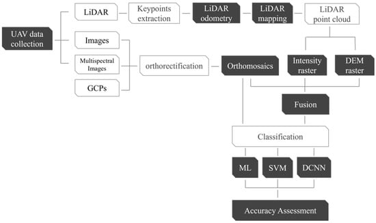
Figure 1.
Workflow of the proposed methodology.
2.1. Orthomosaic Image Generation
An orthomosaic image is an undistorted 2D map composed of multiple overlapped images and corrected for perspective and scale [38]. Pix4D mapper software was used to process the images and create an orthomosaic image. Pix4D uses the principles of photogrammetry to produce an orthomosaic image from input images [39]. The software starts by extracting and matching key points in a series of overlapping images using the SIFT algorithm [40]. Ideally, the overlap between images should be sufficient to specify a single key point in multiple images. To generate a high-quality and accurate orthomosaic through Pix4D software, it is recommended to acquire a series of nadir images with a minimum overlap of 75% [38]. Based on the matched key points and the ground control points (GCPs), the software estimates the interior and exterior orientation parameters of the camera using the triangulation technique followed by bundle adjustment [41]. In order to obtain a DSM, the key points are triangulated to their 3D coordinates. Then, the DSM is used to project every image pixel and create the georeferenced orthomosaic.
2.2. Optimized LOAM SLAM
LiDAR data were processed using an optimized simultaneous localization and mapping (SLAM) technique based on the LiDAR odometry and mapping (LOAM) developed by Kitware [42,43]. Two python nodes (pc saver and traj saver) were developed to subscribe to the trajectory and the point cloud topics and save their outputs. The optimized LOAM SLAM is composed of three main sequential steps, namely, key point extraction, LiDAR odometry, and LiDAR mapping.
In the first step, the key points are classified as edges and planar points based on curvature. Edge points correspond to points with maximum curvature, while planar points correspond to points with minimum curvature. Figure 2 shows an example of the extracted key points of one LiDAR frame. In the LiDAR odometry step, the iterative closest point matching technique [44] is used between two successive frames to recover the LiDAR motion. Depending on the feature type, the point to line distance or point to plane distance can be computed. Finally, the recovered motion is refined by projecting and matching the current frame with the existing map.

Figure 2.
An example of extracted key points: (a) A single LiDAR frame; and (b) Extracted edges (red) and planes (blue).
2.3. Conventional Maximum Likelihood Classifier
Maximum likelihood is one of the most widely used methods in the application of remote sensing as a parametric statistical method [45,46]. ML assumes that data in each class are normally distributed and follow a second-order Gaussian probability density function model [47]. The discriminant function for each class according to the maximum likelihood classifier is given by the following formula [47]:
where is the probability of class ; is the number of bands; is the data vector; is the mean vector of class ; is the covariance matrix. The mean vector and the covariance matrix are estimated from the training data. ML calculates the discriminant function for each class and subsequently assigns the pixel to the class with the highest probability.
2.4. Support Vector Machine Classifier
The support vector machine (SVM) model is a high-performing supervised non-parametric classifier based on statistical machine learning theory and optimal separating hyperplane [48]. This classifier aims to distinguish between classes using training samples by finding the optimal classification hyperplane for a maximum of the classification margin in a feature space. The optimal classification hyperplane is used as a decision boundary, which minimizes misclassifications obtained in the training step. Finding a classifier with an optimal decision boundary is done through a learning iterative process to separate the training patterns [49].
During the process of the SVM, the classification hyperplane is the probable plane for separating the classes . A classification hyperplane can be created using the following equation [48]:
where is a coefficient vector, is the classes vector, and is a scalar. The two parameters of the classification hyperplane decision function, and , can be obtained by solving the following optimization problem:
where and signify the positive slack variable and the penalty parameters of the errors, respectively.
2.5. DCNN Architecture
The DCNN used in this work is the improved version of the U-net model [34], where the Resnet101 [50] network was used as a backbone to extract features. The encoder starts with a 2D convolutional layer with a kernel size of 7 × 7 and stride of 2, followed by a batch normalization (BN) layer, a rectified linear unit (ReLU) layer, and a 2D convolutional layer. The 2D convolutional layer is connected to repeated residual blocks, which consist of BN, ReLU, and convolutional layers. The decoder consists of repeating upsampling layers connected to a concatenate layer and residual blocks, which double the spatial resolutions of the output activations while reducing the number of feature channels by half. The network was built using segmentation models [51], i.e., a python library for image segmentation based on the Keras framework. The total parameters of the network are approximately 52 million. The dice coefficient loss function was used to overcome the imbalance between classes [52]. The following formula determines the dice coefficient loss:
where is the dice coefficient loss, represents the ground truth, and P represents the prediction result of the network. The AMSgrad optimizer was used to minimize the loss function [53]. This optimization algorithm is a modified version of the Adam optimizer [54], which uses the maximum of exponential moving averages of past squared gradients. The AMSGrad update estimates can be estimated as follows:
where and are the first- and second-moment, respectively; is the gradient, which represents the vector of partial derivative with respect to ; is the parameter update; is the learning rate. The hyperparameters and were set to 0.9 and 0.999, respectively, while the epsilon number () was set to 10−7, as typically recommended in practice [53]. The learning rate schedular was used instead of a constant learning rate, which gradually updates the learning rate if the loss plateaued or after a fixed number of epochs to attain the optimum convergence by the end of the training data. Random image augmentations were applied to increase the size of the training data. Tensorflow and Keras were used to implement the network [55,56].
2.6. Accuracy Assessment
Four evaluation metrics were used in the evaluation of the maximum likelihood classification results, i.e., class producer’s accuracy (PA), class user’s accuracy (UA), overall accuracy (OA), and the kappa coefficient. The PA shows what percentage of a particular ground reference class was correctly classified. The UA provides the user of the map with the percentage of a class that corresponds to the ground-truth class. Finally, OA is the percentage of pixels that were classified correctly, while the kappa measures the agreement or accuracy between the derived classification map and the reference data. These values can be calculated based on the following formulas:
where is the total number of ground truth samples; is the number of classes; is the number of correctly classified samples in the land-cover class ; is the total number of ground truth samples in the land-cover class ; is the total number of samples classified as land-cover class .
OA, precision (Pr), recall (R), and the F-measure were used to assess the performance of the DCNN segmentation technique. The precision represents the ratio of the pixels correctly predicted to all pixels predicted. The recall indicates the ratio of the pixels correctly predicted to the total ground truth pixels. The F-measure is the weighted average of precision and recall, which is used when there is a severe class imbalance. The calculation formulas for the performance metrics are as follows:
where TP is the true positive; FP is the false positive; FN is the false negative.
3. Data Acquisition and Preprocessing
In this study, a UAV was used as the platform for imagery and LiDAR data acquisition. Two datasets were collected at two different times and locations in the Toronto, Ontario, which is the most populated city in Canada. The first dataset was used to train the model, while the second dataset was used to validate it. The first dataset was collected in February 2020 using the DJI Matrice 600 Pro UAV, with a payload consisting of a Sony α7R II RGB camera, MicaSense RedEdge-M multispectral camera, and a Velodyne VLP-16 LiDAR sensor. The Sony α7R II camera has a 42 MP spatial resolution with a 7952 × 5304 image size [57]. The MicaSense RedEdge-M camera has five bands, namely, blue, green, red, near-infrared (around 840 nm), and red edge (around 717 nm). The RedEdge-M camera has a 1.2 MP spatial resolution with a 1280 × 960 image size [58]. The Velodyne VLP-16 consists of 16 laser beams with a 360° horizontal field of view (FOV) and a 30° vertical field of view. The maximum range measurement for the VLP-16 is 100 m with a ±3 cm range accuracy [59]. In order to cover the area of interest, the flight was performed in about 9 min with approximately 25 m flight height, acquiring the data in 5 parallel flight lines. The average surface area surveyed was approximately 9000 m2. Figure 3 shows a top view of the flight trajectory over the area of interest. The LiDAR data were acquired at a 10 Hz frame rate with only the maximum return recorded, and the total number of acquired points was approximately 14 million. The number of captured images was 243 images for the RGB camera and 282 images per band for the RedEdge-M camera.
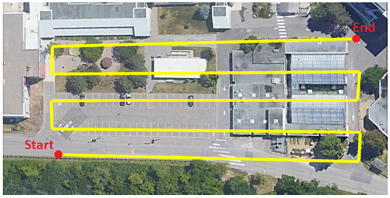
Figure 3.
UAS flight lines above the first test site.
As shown in Figure 4, eight checkerboard targets were deployed at the study site (solid red boxes). The precise (centimeter-level) coordinates of the targets were determined using a dual-frequency SOKKIA GCX2 GPS receiver in the real-time kinematic (RTK) mode. These targets were used as ground control points (GCPs) to georeference the collected images, as there was an issue with the onboard GPS receiver. Later, four GCPs were collected with a Trimble R9s GNSS receiver to improve the geometric distribution of the GCPs (solid yellow boxes). The four new points were processed using Trimble business center (TBC) software in the differential mode with a virtual reference station (VRS) to determine their precise coordinates.
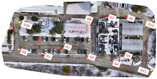
Figure 4.
First study area with red and yellow squares highlighting the GCP positions. G1 through G12 represent the ground control points (GCPs) and check points.
The second dataset was collected in June 2022 using the DJI Zenmuse L1 system carried by a DJI Matrice 300 UAV, which integrates a Livox solid-state Lidar module, GNSS receiver, an IMU, and an RGB camera [60]. The camera has a 20 MP spatial resolution with a 5472 × 3078 image size. The solid-state LiDAR has a 70.4° horizontal field of view (FOV) and a 77.2° vertical field of view. The maximum range measurement is 450 m with a ±3 cm @ 100 m range accuracy. In order to cover the area of interest, the flight was performed in about 5 min with approximately 60 m flight height, acquiring the data in 7 parallel flight lines. The average surface area surveyed was approximately 76,000 m2. Figure 5 shows a top view of the flight trajectory over the second area of interest. The total number of acquired points using the solid-state LiDAR was approximately 42 million. The number of captured images was 208 for the RGB camera. Fifteen checkerboard targets were deployed at the study site. The precise (centimeter-level) coordinates of the targets were determined using a Trimble R8s GNSS receiver in the RTK mode. These targets were used as GCPs to georeference the collected images. In addition, during the data acquisition, a D-RTK 2 GNSS mobile station was fixed on a known GCP to provide real-time differential corrections to the onboard GNSS RTK receiver to georeference the acquired data.
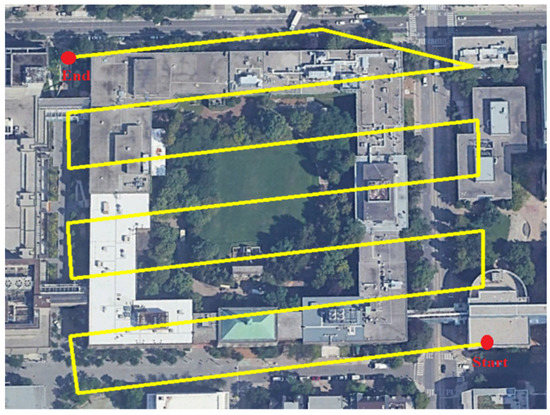
Figure 5.
UAS flight lines above the second test site.
3.1. Data Processing of the First Dataset
The RGB images were processed with the 12 GCPs using Pix4D mapper software to create a georeferenced orthomosaic image, as shown in Figure 6. The same procedures were followed to create georeferenced orthomosaic images of the five multispectral camera bands, as shown in Figure 7. Then, those orthomosaic images were stacked together using ERDAS IMAGINE software to create a single multispectral image (Figure 8) in the false color combination. The band combination adopted for the false color combination was near-infrared (red), green (blue), and red (green). The LiDAR data were processed using optimized LOAM SLAM software, which was executed on a robot operating system (ROS) in a Linux system. Figure 9 and Figure 10 show the LiDAR SLAM trajectory and the generated point cloud, respectively. The LiDAR point cloud was then processed using ArcGIS software without preprocessing (i.e., denoising) to create a DSM and intensity rasters, as shown in Figure 11 and Figure 12, respectively.
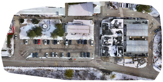
Figure 6.
RGB orthomosaic image for the first test site.

Figure 7.
Five bands orthomosaic images of the multispectral camera for the first test site.
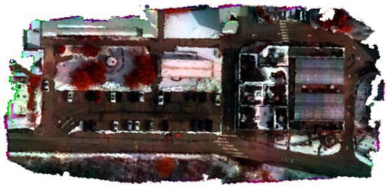
Figure 8.
False-color combination of the multispectral orthomosaic for the first test site.
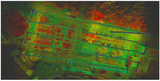
Figure 9.
LiDAR SLAM trajectory for the first test site.
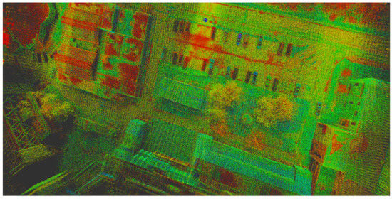
Figure 10.
LiDAR point cloud generated using SLAM for the first test site.
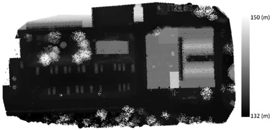
Figure 11.
DSM raster generated using the LiDAR data point cloud for the first test site.
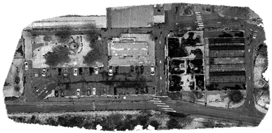
Figure 12.
Intensity raster generated using the LiDAR data point cloud for the first test site.
Six different imaging/LiDAR combinations were created, namely, RGB, RGB + intensity, RGB + elevation, RGB + LiDAR, Multispectral, and Multispectral + elevation. RGB refers to the colored orthomosaic image created using the RGB images, while Multispectral refers to the orthomosaic image created using the multispectral images. The intensity and elevation refer to the intensity and DSM rasters created using the LiDAR data. In the second combination, the intensity was added to RGB as a fourth channel using the layer stacking technique in ERDAS IMAGINE software. Similarly, in the third and the sixth combinations, the elevation was added to RGB as a fourth channel and to the Multispectral as a sixth channel, respectively. Finally, in the fourth combination, the intensity and elevation were added to RGB as fourth and fifth channels, respectively. The fused image of the fourth case is shown in a false color combination in Figure 13. In order to create the ground truth for the DCNN training and validation, 25 subset images were labeled using open-source software called “Labelme” [61]. An example of an image and its ground truth is shown in Figure 14.
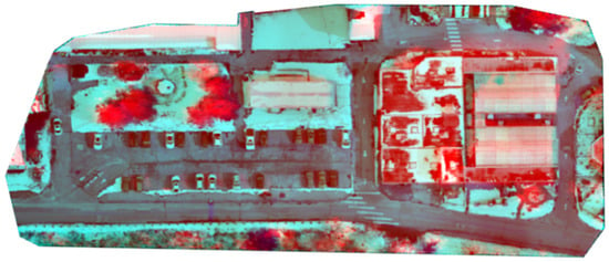
Figure 13.
False-color combination of the RGB + LiDAR case for the first test site.

Figure 14.
Labeled sample using Labelme software.
3.2. Data Processing of the Second Dataset
Similar to the first dataset, the RGB images were processed with the 15 GCPs using Drone2Map software to create a georeferenced orthomosaic image, as shown in Figure 15. The solid-state LiDAR data were processed using DJI Terra software to create a full georeferenced point cloud of the area of interest. The LiDAR point cloud was then processed using ArcGIS software to create a DSM and intensity rasters, as shown in Figure 16 and Figure 17, respectively. Finally, the intensity and DSM rasters were added to RGB orthomosaic as fourth and fifth channels, respectively. The fused image is shown in a false color combination in Figure 18. In order to validate the DCNN model, four different imaging/LiDAR combinations were created, namely, RGB, RGB + intensity, RGB + elevation, and RGB + LiDAR. Subsequently, eight subset images were created and labeled using Labelme.
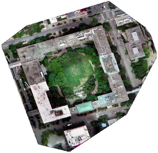
Figure 15.
The RGB orthomosaic image for the second test site.
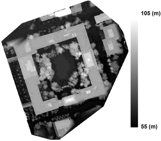
Figure 16.
DSM raster generated using the solid-state LiDAR data point cloud for the second test site.
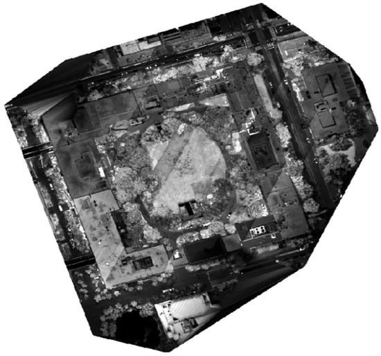
Figure 17.
Intensity raster generated using the solid-state LiDAR data point cloud for the second test site.
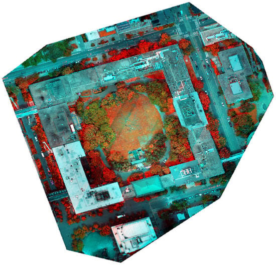
Figure 18.
False-color combination of the fused image for the second test site.
4. Results and Discussion
All six combinations of the first dataset were classified using the maximum likelihood and SVM techniques using the ERDAS IMAGIN and ArcGIS software packages, respectively. Six land cover classes, i.e., “building”, “road”, “vegetation”, “snow”, “cars”, and “unclassified”, were identified. The classification results of both techniques for all combinations are shown in Figure 19 and Figure 20. In order to assess the classification results, 500 random reference points were identified, and error matrices were generated. Then, the evaluation metrics were calculated including PA, UA, OA, and the kappa coefficient. Table 1 and Table 2 show the comparison results of the six combinations for the ML and SVM techniques, respectively.
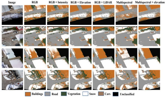
Figure 19.
Classification results using the maximum likelihood technique.
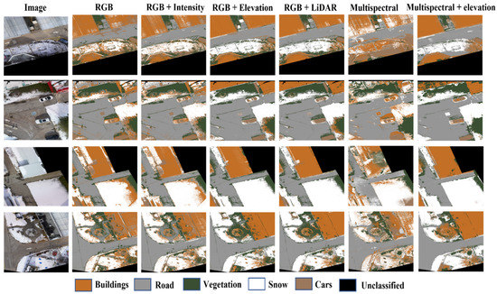
Figure 20.
Classification results using the SVM technique.

Table 1.
Classification results of the six combinations using the maximum likelihood technique.

Table 2.
Classification results of the six combinations using the SVM technique.
As can be seen in Figure 19, in the RGB case, many buildings’ pixels were misclassified as snow and vegetation. For example, the building in the fourth image was misclassified as vegetation. The pixels misclassified as vegetation were decreased by the fusion of the intensity image with the RGB image because of the sensitivity of vegetation to the near-infrared band, as shown in the same example. The UA of vegetation increased by 8% and the OA increased by 7% compared to the RGB case. The addition of the elevation layer improved the building classification accuracy significantly, where the UA was increased by 40% compared to the RGB case. This is mainly because the elevation information differentiates between the snow on the ground and the snow on the building’s rooftop. The LiDAR/image data fusion obtained the best classification result using the ML classifier, with the OA (82%) and kappa coefficient (75%). The Multispectral case produced the worst classification result, where the OA and kappa coefficient were 58% and 40%, respectively. This poor classification accuracy could be explained by the low spatial resolution of the RedEdge-M camera. However, when the LiDAR elevation data were added to the multispectral image, the OA was improved by 20% and the kappa coefficient increased by 30%, which emphasizes the importance of the LiDAR/image data fusion.
The ML and SVM results were very similar; nevertheless, the SVM was superior in all scenarios with about a 2% increase in the OA and kappa coefficient except for one case. It achieved a 69.40% OA versus 70.40% for the ML in the RGB + intensity scenario. These results are consistent with those in previous studies [62,63]. In [62], ML and SVM were compared for land cover classification using satellite images. The OA mean of SVM was 90.40 (±0.91)%, and ML was 87.54 (±1.39)%, with 2.9% difference. As concluded in [63], ML performs better when classifying images in special spectrums such as urban areas, even though more advanced machine learning methods such as SVM offer more accurate image classification in the presence of different classes.
The DCNN was trained and tested on the 25-image subsets of the first dataset for the four RGB different combinations. The 25-image samples were divided into 15 training, 6 validation, and 4 testing images. Figure 21 and Figure 22 illustrate the training and validation accuracy and loss curves of the RGB and RGB + LiDAR cases, respectively. The RGB + LiDAR validation curves were more stable than the RGB case and reached higher accuracy, which means that the addition of LiDAR data improved the generalization of the DCNN model. Figure 23 shows the prediction results of the testing dataset for the four different combinations. Table 3 shows the comparison results of the four combinations in the testing dataset. For the RGB case, the obtained OA was 90%, and the precision, recall, and F-measure were about 72%. Further, due to the similarities in the spectral characteristics of the buildings’ rooftops and the roads, some buildings were misclassified as roads in the RGB case, as shown in Figure 23. Similarly, some ground snow cover was misclassified as buildings as some buildings’ rooftops were covered with snow. The OA of the RGB + LiDAR case was 7% higher than the RGB case, while the precision, recall, and F-measure were 18% higher.
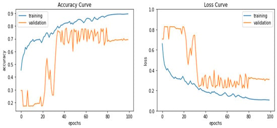
Figure 21.
Training and validation curves of accuracy and loss for the RGB case.
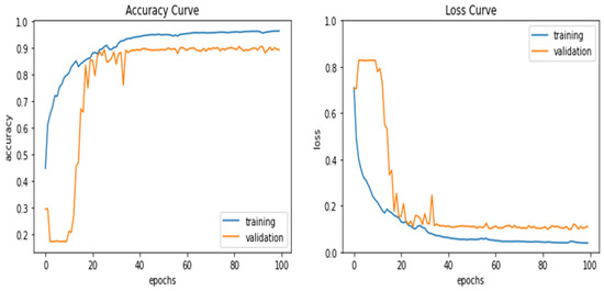
Figure 22.
Training and validation curves of accuracy and loss for the RGB + LiDAR case.
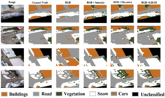
Figure 23.
Comparison of the DCNN prediction results of the first dataset.

Table 3.
Comparison of indicator parameters for the four combinations using DCNN.
To validate and assess the performance of the trained model, the DCNN was tested on the eight image subsets of the second dataset for the four different combinations. Figure 24 shows the prediction results of the validation dataset for the four different combinations. Table 4 shows the comparison results of the four combinations in the validation dataset.
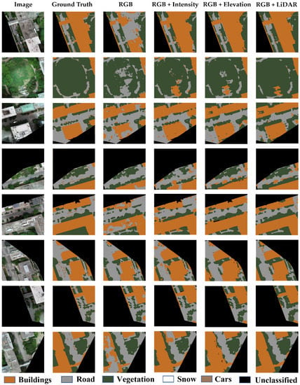
Figure 24.
Comparison of the DCNN prediction results of the second dataset.

Table 4.
Comparison of indicator parameters for the four combinations using DCNN.
Overall, the results obtained from the validation dataset were largely similar to the results of the first dataset. However, the accuracy of the RGB case was increased by 3%, while the precision, recall, and F-measure were increased by 8% compared to the first dataset. This increase is likely due to the seasonal variations, where the first dataset was collected in the winter with the ground partially covered by the snow, while the second dataset was collected in the spring. For example, the snow covering the rooftop of the building affected the classification accuracy of the first dataset. As can be noticed in the third image of the RGB case in Figure 23, the ground snow was misclassified as buildings. The integration of image/LiDAR data overcame these seasonal variations, as can be seen in the three other cases of the same image. Therefore, the results of the fused data cases in the validation dataset were slightly better compared to the first dataset.
Figure 25 compares the overall classification accuracy of the ML and SVM with the DCNN approach for the four investigated combinations of both datasets. The use of DCNN improved the OA by about 30% in the RGB case and by 15% in the RGB + LiDAR case compared to the ML and SVM techniques.
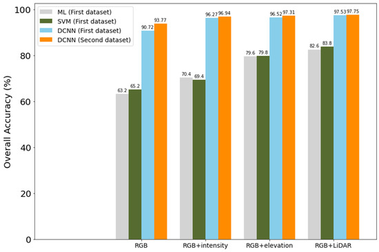
Figure 25.
Overall accuracy comparison between the ML and the DCNN.
5. Conclusions
In this research, a low-cost UAS-based multi-sensor data fusion model was developed for land cover classification based on DCNN. Two datasets were collected to train and validate the developed model. The first dataset was collected using a DJI Matrice-600 UAV with a payload that included the Velodyne VLP-16 mechanical LiDAR sensor, the Sony a7Rii camera, and RedEdge-M multispectral camera. The second dataset was collected using the DJI Zenmuse L1, which combines a solid-state LiDAR sensor, an RGB camera, an IMU, and a GNSS receiver. The DCNN approach was based on U-net with Resnet101 as a backbone, which has about 52 million parameters. The first dataset was used to train the DCNN, while the second dataset was used to validate the model. The model was trained on six land cover classes, namely, “building”, “road”, “vegetation”, “snow”, “cars”, and “unclassified”. The results obtained from the DCNN approach were compared to those obtained from the ML and SVM techniques.
The ML and SVM techniques obtained very similar classification results. The image/LiDAR data fusion improved the classification accuracy by about 20% and the kappa coeffcieint by about 25% in comparison with the image-only data. The proposed DCNN approach improved the overall accuracy of land cover classification by 30% in the RGB case and by 15% in the RGB + LiDAR case in comparison with the ML and SVM classification techniques. The overall accuracy of land cover classification using DCNN improved by 7%, and the precision, recall, and F-measure improved by 18% when the fused image/LiDAR data were used compared to image-only data. In addition, the image/LiDAR data fusion overcame the effect of seasonal variations on the land cover classification accuracy. The results of the validation dataset supported the outcomes of the trained DCNN model. The obtained results confirm that the proposed approach is capable of providing accurate land cover classification at low cost.
Author Contributions
Conceptualization: A.E.-R. and A.E.; methodology: A.E.; software: A.E.; validation: A.E.; formal analysis: A.E.; writing—original draft preparation, A.E.; writing—review and editing: A.E.-R.; supervision, A.E.-R. All authors have read and agreed to the published version of the manuscript.
Funding
This research is supported by Toronto Metropolitan University and Natural Sciences and Engineering Research Council of Canada (NSERC) RGPIN-2022-03822.
Data Availability Statement
The data presented in this study are not publicly available.
Acknowledgments
The authors would like to thank Akram Afifi, a professor in the Faculty of Applied Sciences and Technology, Humber College, for providing the first dataset used in this research. Jimmy Tran and Dan Jakubek of TMU Library are thanked for collecting the dataset and making it available for this study. The authors would also like to thank Kitware for making its SLAM package available.
Conflicts of Interest
The authors declare no conflict of interest.
References
- Yifang, B.; Gong, P.; Gini, C. Global land cover mapping using Earth observation satellite data: Recent progresses and challenges. ISPRS J. Photogramm. Remote Sens. 2015, 103, 1–6. [Google Scholar]
- Feddema, J.J.; Oleson, K.W.; Bonan, G.B.; Mearns, L.O.; Buja, L.E.; Meehl, G.A.; Washington, W.M. The Importance of Land-Cover Change in Simulating Future Climates. Science 2005, 310, 1674–1678. [Google Scholar] [CrossRef] [PubMed]
- Raid Al-Tahir, M.A. Unmanned Aerial Mapping Solution for Small Island Developing States. In Proceedings of the global geospatial conference, Quebec City, QC, Canada, 17 May 2012. [Google Scholar]
- Kalantar, B.; Halin, A.A.; Al-Najjar HA, H.; Mansor, S.; van Genderen, J.L.; Shafri HZ, M.; Zand, M. A Framework for Multiple Moving Objects Detection in Aerial Videos, in Spatial Modeling in GIS and R for Earth and Environmental Sciences; Elsevier: Amsterdam, The Netherlands, 2019; pp. 573–588. [Google Scholar]
- Yao, H.; Qin, R.; Chen, X.J.R.S. Unmanned aerial vehicle for remote sensing applications—A review. Remote Sens. 2019, 11, 1443. [Google Scholar] [CrossRef]
- Torresan, C.; Berton, A.; Carotenuto, F.; Di Gennaro, S.F.; Gioli, B.; Matese, A.; Miglietta, F.; Vagnoli, C.; Zaldei, A.; Wallace, L. Forestry applications of UAVs in Europe: A review. Int. J. Remote Sens. 2017, 38, 2427–2447. [Google Scholar] [CrossRef]
- Lv, Z.; Shi, W.; Benediktsson, J.A.; Ning, X. Novel object-based filter for improving land-cover classification of aerial imagery with very high spatial resolution. Remote Sens. 2016, 8, 1023. [Google Scholar] [CrossRef]
- Natesan, S.; Armenakis, C.; Benari, G.; Lee, R. Use of UAV-Borne Spectrometer for Land Cover Classification. Drones 2018, 2, 16. [Google Scholar] [CrossRef]
- Giang, T.L.; Dang, K.B.; Le, Q.T.; Nguyen, V.G.; Tong, S.S.; Pham, V.M. U-Net convolutional networks for mining land cover classification based on high-resolution UAV imagery. IEEE Access 2020, 8, 186257–186273. [Google Scholar] [CrossRef]
- Pan, L.; Gu, L.; Ren, R.; Yang, S. Land cover classification based on machine learning using UAV multi-spectral images. SPIE 2020, 11501, 115011F. [Google Scholar]
- Park, G.; Park, K.; Song, B.; Lee, H. Analyzing Impact of Types of UAV-Derived Images on the Object-Based Classification of Land Cover in an Urban Area. Drones 2022, 6, 71. [Google Scholar] [CrossRef]
- Long, T.; Jiao, W.; He, G.; Zhang, Z.; Cheng, B.; Wang, W. A generic framework for image rectification using multiple types of feature. ISPRS J. Photogramm. Remote Sens. 2015, 102, 161–171. [Google Scholar] [CrossRef]
- Megahed, Y.; Shaker, A.; Sensing, W.Y.-R. Fusion of Airborne LiDAR Point Clouds and Aerial Images for Heterogeneous Land-Use Urban Mapping. Remote Sens. 2021, 13, 814. [Google Scholar] [CrossRef]
- Fieber, K.D.; Davenport, I.J.; Ferryman, J.M.; Gurney, R.J.; Walker, J.P.; Hacker, J.M. Analysis of full-waveform LiDAR data for classification of an orange orchard scene. ISPRS J. Photogramm. Remote Sens. 2013, 82, 63–82. [Google Scholar] [CrossRef] [Green Version]
- Reese, H.; Nyström, M.; Nordkvist, K.; Olsson, H. Combining airborne laser scanning data and optical satellite data for classification of alpine vegetation. Int. J. Appl. Earth Obs. Geoinfor. ITC J. 2013, 27, 81–90. [Google Scholar] [CrossRef]
- Tonolli, S.; Dalponte, M.; Neteler, M.; Rodeghiero, M.; Vescovo, L.; Gianelle, D. Fusion of airborne LiDAR and satellite multispectral data for the estimation of timber volume in the Southern Alps. Remote Sens. Environ. 2011, 115, 2486–2498. [Google Scholar] [CrossRef]
- Dalponte, M.; Bruzzone, L.; Gianelle, D. Tree species classification in the Southern Alps based on the fusion of very high geometrical resolution multispectral/hyperspectral images and LiDAR data. Remote Sens. Environ. 2012, 123, 258–270. [Google Scholar] [CrossRef]
- Buddenbaum, H.; Seeling, S.; Hill, J. Fusion of full-waveform lidar and imaging spectroscopy remote sensing data for the characterization of forest stands. Int. J. Remote Sens. 2013, 34, 4511–4524. [Google Scholar] [CrossRef]
- Mutlu, M.; Popescu, S.C.; Stripling, C.; Spencer, T. Mapping surface fuel models using lidar and multispectral data fusion for fire behavior. Remote Sens. Environ. 2008, 112, 274–285. [Google Scholar] [CrossRef]
- Bork, E.W.; Su, J.G. Integrating LIDAR data and multispectral imagery for enhanced classification of rangeland vegetation: A meta analysis. Remote Sens. Environ. 2007, 111, 11–24. [Google Scholar] [CrossRef]
- Mesas-Carrascosa, F.J.; Castillejo-González, I.L.; de la Orden, M.S.; Porras, A.G.-F. Combining LiDAR intensity with aerial camera data to discriminate agricultural land uses. Comput. Electron. Agric. 2012, 84, 36–46. [Google Scholar] [CrossRef]
- Myint, S.W.; Gober, P.; Brazel, A.; Grossman-Clarke, S.; Weng, Q. Per-pixel vs. object-based classification of urban land cover extraction using high spatial resolution imagery. Remote Sens. Environ. 2011, 115, 1145–1161. [Google Scholar] [CrossRef]
- Blaschke, T.; Lang, S.; Lorup, E.; Strobl, J.; Zeil, P. Object-oriented image processing in an integrated GIS/remote sensing environment and perspectives for environmental applications. Environ. Inf. Plan. Politics Public 2000, 2, 555–570. [Google Scholar]
- Zhang, P.; Ke, Y.; Zhang, Z.; Wang, M.; Li, P.; Zhang, S. Urban land use and land cover classification using novel deep learning models based on high spatial resolution satellite imagery. Sensors 2018, 18, 3717. [Google Scholar] [CrossRef]
- Ke, Y.; Quackenbush, L.J.; Im, J. Synergistic use of QuickBird multispectral imagery and LIDAR data for object-based forest species classification. Remote Sens. Environ. 2010, 114, 1141–1154. [Google Scholar] [CrossRef]
- Li, D.; Ke, Y.; Gong, H.; Li, X. Object-Based Urban Tree Species Classification Using Bi-Temporal WorldView-2 and WorldView-3 Images. Remote Sens. 2015, 7, 16917–16937. [Google Scholar] [CrossRef]
- Duro, D.C.; Franklin, S.E.; Dubé, M.G. A comparison of pixel-based and object-based image analysis with selected machine learning algorithms for the classification of agricultural landscapes using SPOT-5 HRG imagery. Remote Sens. Environ. 2012, 118, 259–272. [Google Scholar] [CrossRef]
- Huang, B.; Zhao, B.; Song, Y. Urban land-use mapping using a deep convolutional neural network with high spatial resolution multispectral remote sensing imagery. Remote Sens. Environ. 2018, 214, 73–86. [Google Scholar] [CrossRef]
- Audebert, N.; Le Saux, B.; Lefèvre, S. Semantic segmentation of earth observation data using multimodal and multi-scale deep networks. In Proceedings of the Asian Conference on Computer Vision, Taipei, Taiwan, 20–24 November 2016. [Google Scholar]
- Kemker, R.; Salvaggio, C.; Kanan, C. Algorithms for semantic segmentation of multispectral remote sensing imagery using deep learning. ISPRS J. Photogramm. Remote Sens. 2018, 145, 60–77. [Google Scholar] [CrossRef]
- Zheng, C.; Wang, L. Semantic segmentation of remote sensing imagery using object-based Markov random field model with regional penalties. IEEE J. Sel. Top. Appl. Earth Obs. Remote Sens. 2014, 8, 1924–1935. [Google Scholar] [CrossRef]
- Pinheiro, P.O.; Lin, T.Y.; Collobert, R.; Dollár, P. Learning to refine object segments. In European Conference on Computer Vision; Springer: Berlin/Heidelberg, Germany, 2016. [Google Scholar]
- Lin, G.; Milan, A.; Shen, C.; Reid, I. Refinenet: Multi-path refinement networks for high-resolution semantic segmentation. In Proceedings of the IEEE Conference on Computer Vision and Pattern Recognition, Honolulu, HI, USA, 21–26 July 2017. [Google Scholar]
- Ronneberger, O.; Fischer, P.; Brox, T. U-net: Convolutional networks for biomedical image segmentation. In International Conference on Medical Image Computing and Computer-Assisted Intervention; Springer: Berlin/Heidelberg, Germany, 2015. [Google Scholar]
- Jakovljevic, G.; Govedarica, M.; Alvarez-Taboada, F. A Deep Learning Model for Automatic Plastic Mapping Using Unmanned Aerial Vehicle (UAV) Data. Remote Sens. 2020, 12, 1515. [Google Scholar] [CrossRef]
- Diakogiannis, F.I.; Waldner, F.; Caccetta, P.; Wu, C. ResUNet-a: A deep learning framework for semantic segmentation of remotely sensed data. ISPRS J. Photogramm. Remote Sens. 2020, 162, 94–114. [Google Scholar] [CrossRef]
- Garg, L.; Shukla, P.; Singh, S.; Bajpai, V.; Yadav, U. Land Use Land Cover Classification from Satellite Imagery using mUnet: A Modified Unet Architecture. VISIGRAPP 2019, 4, 359–365. [Google Scholar]
- Hawkins, S. Using a drone and photogrammetry software to create orthomosaic images and 3D models of aircraft accident sites. In Proceedings of the ISASI 2016 Seminar, Reykjavik, Iceland, 17–21 October 2016. [Google Scholar]
- Mapper, P.D. 2020. Available online: https://cloud.pix4d.com/ (accessed on 7 October 2020).
- Lowe, D.G. Distinctive Image Features from Scale-Invariant Keypoints. Int. J. Comput. Vis. 2004, 60, 91–110. [Google Scholar] [CrossRef]
- Küng, O.; Strecha, C.; Beyeler, A.; Zufferey, J.-C.; Floreano, D.; Fua, P.; Gervaix, F. The Accuracy of Automatic Photogrammetric Techniques on Ultra-Light UAV Imagery. In Proceedings of the IAPRS, International Conference on Unmanned Aerial Vehicle in Geomatics (UAV-g), Zurich, Switzerland, 14–16 September 2011. [Google Scholar]
- Kitware. Optimized LOAM SLAM. Available online: https://gitlab.kitware.com/keu-computervision/slam (accessed on 1 March 2020).
- Zhang, J.; Singh, S. LOAM: Lidar Odometry and Mapping in Real-time. In Robotics: Science and Systems; MIT Press: Cambridge, MA, USA, 2014. [Google Scholar]
- Rusinkiewicz, S.; Levoy, M. Efficient variants of the ICP algorithm. In Proceedings of the Third International Conference on 3-D Digital Imaging and Modeling, Quebec City, QC, Canada, 28 May–1 June 2001. IEEE. [Google Scholar]
- Randazzo, G.; Cascio, M.; Fontana, M.; Gregorio, F.; Lanza, S.; Muzirafuti, A. Mapping of Sicilian pocket beaches land use/land cover with sentinel-2 imagery: A case study of messina Province. Land 2021, 10, 678. [Google Scholar] [CrossRef]
- Li, Y.; Bai, J.; Zhang, L.; Yang, Z. Mapping and Spatial Variation of Seagrasses in Xincun, Hainan Province, China, Based on Satellite Images. Remote Sens. 2022, 14, 2373. [Google Scholar] [CrossRef]
- Paola, J.; Schowengerdt, R. A detailed comparison of backpropagation neural network and maximum-likelihood classifiers for urban land use classification. IEEE Trans. Geosci. Remote Sens. 1995, 33, 981–996. [Google Scholar] [CrossRef]
- Vapnik, V. The support vector method of function estimation. In Nonlinear Modeling; Springer: Berlin/Heidelberg, Germany, 1998; pp. 55–85. [Google Scholar]
- Mountrakis, G.; Im, J.; Ogole, C. Support vector machines in remote sensing: A review. ISPRS J. Photogramm. Remote Sens. 2011, 66, 247–259. [Google Scholar] [CrossRef]
- He, K.; Zhang, X.; Ren, S.; Sun, J. Deep residual learning for image recognition. In Proceedings of the IEEE conference on computer vision and pattern recognition, Las Vegas, NV, USA, 27–30 June 2016. [Google Scholar]
- Yakubovskiy, P. Segmentation Models. 2019. Available online: https://github.com/qubvel/segmentation_models (accessed on 17 January 2022).
- Milletari, F.; Navab, N.; Ahmadi, S.-A. V-net: Fully convolutional neural networks for volumetric medical image segmentation. In Proceedings of the 2016 Fourth International Conference on 3D Vision (3DV), Stanford, CA, USA, 25–28 October 2016. [Google Scholar]
- Reddi, S.J.; Kale, S.; Kumar, S. On the convergence of adam and beyond. arXiv 2019, arXiv:1904.09237. [Google Scholar]
- Kingma, D.P.; Ba, J. Adam: A method for stochastic optimization. arXiv 2014, arXiv:1412.6980. [Google Scholar]
- TensorFlow. TensorFlow. 2021. Available online: https://www.tensorflow.org/ (accessed on 17 January 2021).
- Chollet, F.K. Keras: Deep Learning for Humans; GitHub: San Francisco, CA, USA, 2015; Available online: https://github.com/keras-team/keras (accessed on 17 January 2021).
- Sony. Sony ILCE-7RM2. 2021. Available online: https://electronics.sony.com/imaging/interchangeable-lens-cameras/full-frame/p/ilce7rm2-b (accessed on 19 September 2021).
- RedEdge-M. MicaSense. 2022. Available online: https://support.micasense.com/hc/en-us/articles/360001485134-Getting-Started-With-RedEdge-M-Legacy- (accessed on 20 January 2022).
- Velodyne. VLP-16 User Manual. 2021. Available online: https://velodynelidar.com/wp-content/uploads/2019/12/63-9243-Rev-E-VLP-16-User-Manual.pdf (accessed on 19 September 2021).
- DJI Zenmuse L1. 2022. Available online: www.dji.com/cz/zenmuse-l1/specs (accessed on 20 June 2021).
- Labelme. Available online: https://github.com/wkentaro/labelme (accessed on 1 February 2022).
- Rimal, B.; Rijal, S.; Kunwar, R. Comparing support vector machines and maximum likelihood classifiers for mapping of urbanization. J. Indian Soc. Remote Sens. 2020, 48, 71–79. [Google Scholar] [CrossRef]
- Ghayour, L.; Neshat, A.; Paryani, S.; Shahabi, H.; Shirzadi, A.; Chen, W.; Al-Ansari, N.; Geertsema, M.; Amiri, M.P.; Gholamnia, M.; et al. Performance evaluation of sentinel-2 and landsat 8 OLI data for land cover/use classification using a comparison between machine learning algorithms. Remote Sens. 2021, 13, 1349. [Google Scholar] [CrossRef]
Publisher’s Note: MDPI stays neutral with regard to jurisdictional claims in published maps and institutional affiliations. |
© 2022 by the authors. Licensee MDPI, Basel, Switzerland. This article is an open access article distributed under the terms and conditions of the Creative Commons Attribution (CC BY) license (https://creativecommons.org/licenses/by/4.0/).