Deep Learning on Synthetic Data Enables the Automatic Identification of Deficient Forested Windbreaks in the Paraguayan Chaco

Abstract

The Paraguayan Chaco is one of the most rapidly deforested areas in Latin America, mainly due to cattle ranching. Continuously forested windbreaks between agricultural areas and forest patches within these areas are mandatory to minimise the impact that the legally permitted logging has on the ecosystem. Due to the large area of the Paraguayan Chaco, comprehensive in situ monitoring of the integrity of these landscape elements is almost impossible. Satellite-based remote sensing offers excellent prerequisites for large-scale land cover analyses. However, traditional methods mostly focus on spectral and texture information while dismissing the geometric context of landscape features. Since the contextual information is very important for the identification of windbreak gaps and central forests, a deep learning-based detection of relevant landscape features in satellite imagery could solve the problem. However, deep learning methods require a large amount of labelled training data, which cannot be collected in sufficient quantity in the investigated area. This study presents a methodology to automatically classify gaps in windbreaks and central forest patches using a convolutional neural network (CNN) entirely trained on synthetic imagery. In a two-step approach, we first used a random forest (RF) classifier to derive a binary forest mask from Sentinel-1 and -2 images for the Paraguayan Chaco in 2020 with a spatial resolution of 10 m. We then trained a CNN on a synthetic data set consisting of purely artificial binary images to classify central forest patches and gaps in windbreaks in the forest mask. For both classes, the CNN achieved an F1 value of over 70%. The presented method is among the first to use synthetically generated training images and class labels to classify natural landscape elements in remote sensing imagery and therewith particularly contributes to the research on the detection of natural objects such as windbreaks.

1. Introduction

The Paraguayan Chaco is a complex ecosystem rich in rare species, and its dry forest is part of the largest dry forest in the world [1]. At the same time, Paraguay is one of the fastest deforested countries in Latin America, and more than 40% of the Paraguayan Chaco’s forest cover has been lost since 1987 [2]. This is a major threat to the conservation of existing flora, fauna and soil conditions. Paraguay’s forestry and environmental authorities try to ensure the protection of the environment through the implementation of environmental laws and resolutions, the basis of which was created in 1986 with Decree 18831/86 [3]. Among other aspects, it prohibits the deforestation of contiguous areas larger than 100 ha and requires that the logged areas be separated by forested stripes at least 100 m wide. These forested stripes primarily serve to preserve forest and protect the soil from wind erosion, which is why they are also referred to as windbreaks in the following. Further regulations concerning a redefinition of the width of windbreaks [4,5] and the protection of the endangered tree species palo santo (Balnessia sarmientoi) [6], were defined in the following years. This resulted in the formation of central forest patches in agricultural fields—a second important landscape feature in the Paraguayan Chaco that shall protect the rare palo santo tree.

Similar regulations also exist in Argentina and define the realization of windbreaks in the Argentinian Chaco [7]. The established rules are important to limit the negative consequences that deforestation has on nature. Windbreaks connect micro-ecosystems by allowing flora and fauna to migrate, and they have a positive influence on the microclimate. They alter the magnitude and direction of wind, which regulates the temperature and moisture of the soils and reduces soil erosion [8,9]. In the lee of windbreaks, the evaporation of surface humidity is reduced, and the surface heats up more than in exposed areas [10]. The warmer and more humid soils, in turn, facilitate chemical and biological mechanisms promoting an increased biological diversity [10]. Moreover, windbreaks can protect soil ecosystems from permanent deterioration as a consequence of droughts and floods [10]. All of the mentioned points reveal the importance of intact forested stripes.

Ginzburg et al. [7] found that less than 40% of the mandatory windbreaks were present in their study area in the Argentinian Chaco in 2012. In Paraguay, too, the environmental regulations are often disregarded, and many of the windbreaks are narrower than they should be, or the farmers cut wide aisles to connect neighbouring fields. Comprehensive monitoring of the windbreaks is necessary. However, there are hardly any paved roads in the Paraguayan Chaco, making it difficult to reach remote areas. In situ monitoring of the environmental resolutions requires days of travel and is only possible selectively, whereas satellite remote sensing can provide exhaustive, repeated, and detailed imagery of remote areas.

Even though the importance of windbreaks is well known, only few publications address the monitoring of windbreaks through remote sensing imagery. Liknes et al. [11] presented a semi-automated, morphology-based approach using binary forest maps to differentiate between different types of windbreaks (i.e., north-south or east-west oriented, or L-shaped). Although their method distinguishes between windbreaks and riparian corridors, it is not applicable if the windbreaks are connected to other forest patches. Different from Liknes et al. [11], most other studies on windbreaks do not classify the windbreaks in an automated manner. To map windbreaks, Burke et al. [12] and Ghimire et al. [13] used the commercial software “eCognition” and the “ENVI Zoom 4.5 Feature Extractor”, respectively, to generate object polygons which they manually optimized in a second step. Piwowar et al. [14] even waived commercial software, concluding that manual labelling is faster than correcting all errors from the software results. Furthermore, Deng et al. work on manual annotations for their analysis on the width [15] and continuity [16] of windbreaks. For the detection of discontinuities, their approach requires vector lines of windbreaks that are continuous over gaps in order to identify the gaps along the line [16]. A more recent publication by Ahlswede et al. [17] reviews the potential of deep learning models to recognize linear woody features such as hedges, which have a similar structure as windbreaks, in satellite imagery and shows promising results reaching an F1 score of 75%. To train the convolutional neural networks (CNNs), they had manually annotated polygons for the individual hedges at their disposal. What all these approaches have in common and what differentiates them from the situation in the Paraguayan Chaco is the fact that they all address isolated windbreaks, well-separated from each other, while grids of connected windbreaks are characteristic for the Paraguayan Chaco. Moreover, most of these publications address much smaller study areas of less than 4000 km${}^2$ (study area Paraguayan Chaco: 240,000 km${}^2$).

In contrast with [7,14,15,16], who manually digitised windbreaks based on forest masks, we aim at an automatic recognition of gaps in windbreaks and of central forest patches in agricultural fields. In the last decade, deep learning has become an important tool in Earth observation [18,19,20,21]. This sub-field of machine learning uses neural networks to analyse large amounts of data by learning suitable feature extractors. The basic structure of neural networks consists of successive layers of adjustable parameters. Here, the increasing depth of the models reflects the possibility of being able to map increasingly complex feature representations. Due to this model layout, with a sufficient amount and variability of training data, deep learning models have the potential to learn complex feature representations from the training data [22]. In particular, CNNs from the computer vision domain for the analysis of image data [22,23] and their further development have led to the consideration of multiscale spatial features [20,24,25,26], which make them the most widely used deep learning model in Earth observation [19,20,21]. As stated above, large and variable training data sets, e.g., sets of images with their corresponding pixel-wise class label, are necessary to optimise a deep learning model sufficiently. Particularly in Earth observation, the acquisition of training data is very time intensive and often requires experts who are skilled in interpreting remote sensing imagery [27,28]. Furthermore, the Paraguayan Chaco is a rather small application area in the deep learning domain. To train a neural network on annotated images from the Paraguayan Chaco, probably the entire region would be needed for training. Additionally, in case of mapping gaps in windbreaks, such labelling is an extremely time-intensive task because each gap needs to be annotated as an individual polygon.

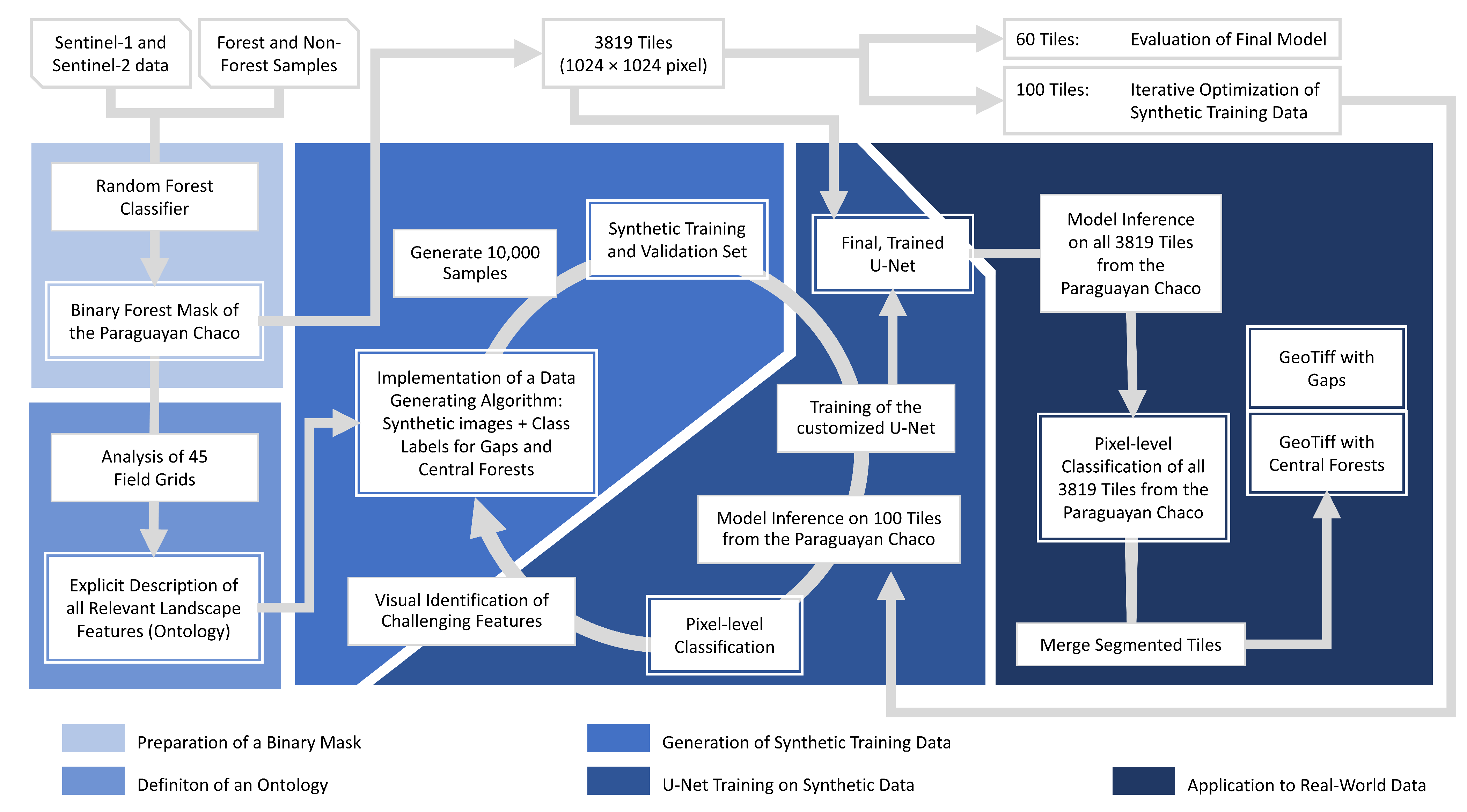
To overcome these limitations, this study uses a deep learning approach and synthetic training data to detect windbreak gaps and central forest patches. Similar to Liknes et al. [11], we conduct the windbreak mapping based on binary forest maps. The forest maps were derived from Sentinel-1 and -2 imagery using an random forest (RF) classification to distinguish between forest and non-forest areas. Consequently, this simplifies the following training of the CNN because it only learns from binary images. Thus, it is widely independent of a specific sensor radiometry, acquisition geometry, and light conditions, and only needs to focus on the spatial features. Additionally, instead of manually labelling heaps of image tiles, we train our CNN on completely synthetically generated training data. This is a novel approach for landscape feature recognition and has, to our knowledge, yet only been applied in one study on natural landscape elements, i.e., [29], and in a few other studies on human-made objects, e.g., [28,30,31]. By using synthetic data, we can not only avoid resource-intensive manual work, but we can also make sure that sufficiently variable and numerous training data are available. For a deep learning model to solve the given task by learning a highly generalised but still accurate representation of the underlying features, we need thousands of different examples. Furthermore, the synthetically generated training data are adjustable, and therewith, it provides the opportunity to control the deep learning model behaviour. In order to systematically embed expert knowledge about the agro-environmental system, spatial features, and the Earth observation sensor, the recently proposed SyntEO framework for synthetic data generation in Earth observation by Hoeser and Kuenzer [28] was used as a strategic guide.

Based on the binary forest map and the synthetic training data set, we aim at mapping deficiencies in windbreaks and central forest patches in an efficient and automated manner in the entire Paraguayan Chaco for the year 2020. At the same time, we would like to demonstrate in this study how the concept of a synthetic training data set can be implemented in the remote sensing domain and reveal this method’s opportunities and limitations.

2. Study Area

The study region of this work is the Paraguayan Chaco, which is located in the western part of Paraguay. It constitutes 25% of the Great American Chaco—a forest region with a subtropical climate spreading over several South American countries [1]. The landscape of the Paraguayan Chaco is dominated by regularly flooded savannahs in the East and the South. In contrast, the central and north-western parts are characterized by dry forests which are, especially in the centre, permeated by agricultural fields. Even though the region comprises more than 60% of the country, having an area of approximately 240,000 km${}^2$, only 3% of the population lives there [1]. At the same time, the Paraguayan Chaco has been identified as one of the regions with the highest rates of deforestation in South America [2,32,33]. Numbers for 2008–2020 show that every year, 3200 km ${}^2$ of the forest is logged [2], whereby the land is subsequently used as pasture in most cases [32,33]. 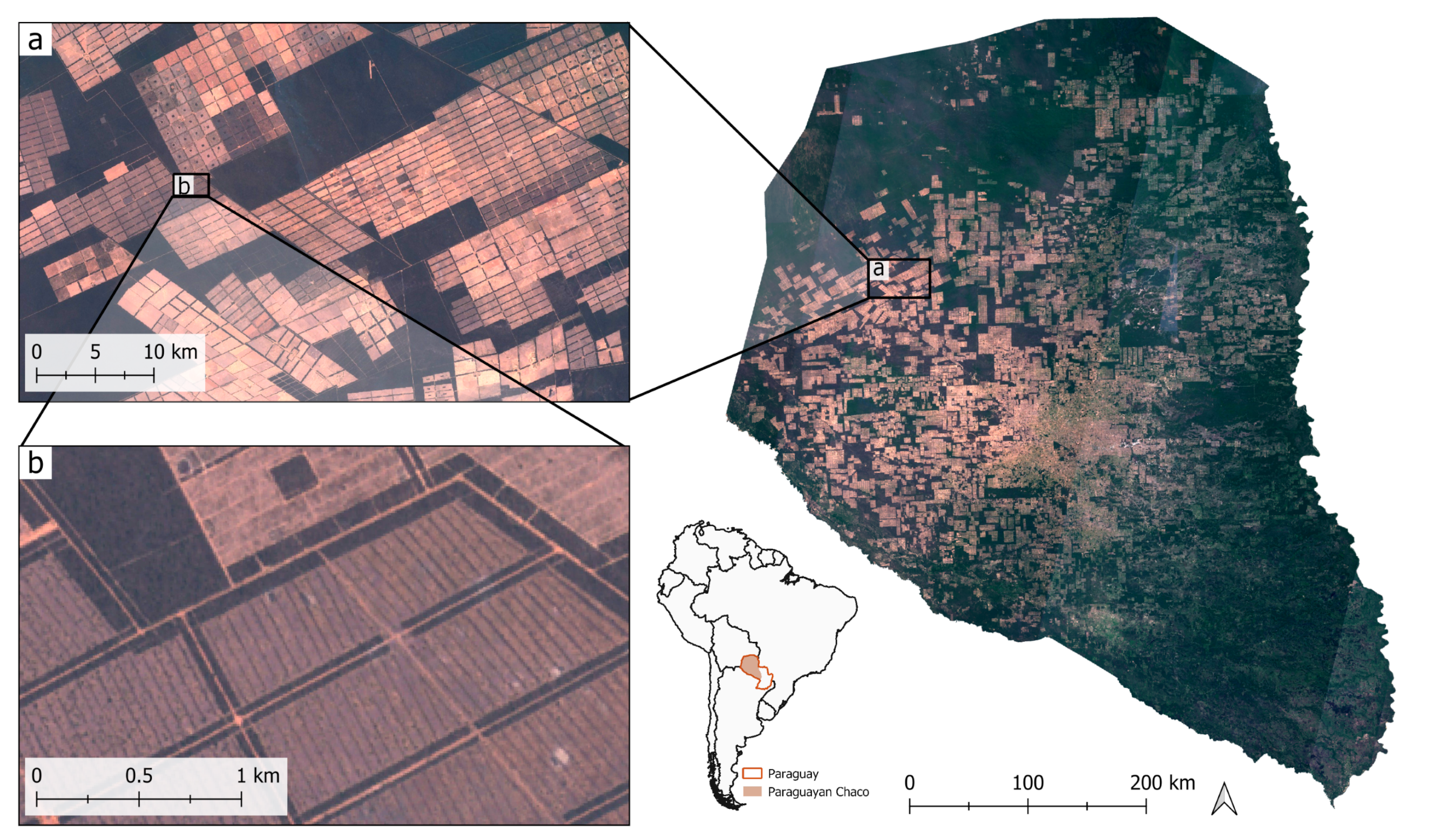Figure 1 shows an overview map of the Paraguayan Chaco with two magnifications of different scales which reveal the typical shape and arrangement of the agricultural areas: rectangular and grid-like. This structure is the result of a decree passed by the Paraguayan government in 1986. It specifies that continuously logged areas must not be larger than 100 ha and that they must be separated from each other by forested stripes with a minimum width of 100 m [3]. Intact forested stripes, also called windbreaks, are essential landscape elements that protect the soil from wind erosion, which is important, since the Paraguayan Chaco is a flat plane with average wind velocities of 16.2 to 24.5 km/h [1]. However, many of these windbreaks are eroded or interrupted, which is depicted in Figure 1b.

3. Materials and Method

This work aims to identify two types of landscape features which are hereafter also addressed as classes: It involves both the detection of forest patches that are centrally located in some of the fields and the detection of gaps in forest stripes that serve as windbreaks. The proposed method for detecting these features comprises five main steps (see Figure 2) which are individually addressed in the following sections: The preparation of a binary forest mask, the transfer of real-world observations of a domain expert to an ontology that is machine-readable, the generation of synthetic training data, the training of the adapted U-Net model on the synthetic data, and the application of the model to remote sensing imagery. We also assessed the model accuracy based on manually labelled imagery from the study area. Figure 2 provides an overview of the entire process. The corresponding detailed description of all steps is shown in Figure 3.

3.1. Generation of the Forest Mask

The classification of forest and non-forest areas is based on a RF model with various spectral features derived from the preprocessed Sentinel-1 and -2 scenes from the year 2020. The data, with a spatial resolution of 10 to 20 m, was obtained and processed in Google Earth Engine [34]. For Sentinel-1, which provides imagery of a C-Band Synthetic-Aperture-Radar (SAR) instrument, we used only descending orbit scenes of the Level-1 Ground-Range-Detected (GRD) product. After filtering the data to VV (vertical sent–vertical received) and VH (vertical sent–horizontal received) polarization, the resulting analysis-ready collection comprised 426 scenes. To reduce the amount of data but still capture the phenological variation, we calculated percentiles (10th, 25th, 50th, 75th, and 90th) of the annual stack of VV and VH polarized images.

From the Multi-Spectral Instrument (MSI) onboard Sentinel-2, we used the Level-1C product with Top-of-Atmosphere (ToA) reflectance and less than 30% cloud coverage. In the resulting 3098 scenes, all remaining clouds were masked through the provided cloud mask of the Level-1C product [35]. The following spectral bands were used for analysis: blue (B2), green (B3), red (B4), near-infrared (B8), short-wave-infrared-1 (B11), and short-wave-infrared-2 (B12) [36]. From this collection, we calculated spectral indices (NDVI, EVI, NDWI [37], and Tasseled Cap Greenness [38]) as additional features, and added them to the selected spectral bands. Similar to the processing of the Sentinel-1 data, we aggregated the annual Sentinel-2 stacks to percentiles of each spectral band or index. In addition, we obtained the differences in percentiles (75th–25th and 90th–10th) from all Sentinel-1 backscatter and Sentinel-2 spectral features, resulting in 74 features in total.

The classification workflow is similar to the study of [2], who aggregated annual Landsat data for long multitemporal forest cover change analysis in Paraguay. Modelling has been conducted in two steps: Following a feature importance analysis of all 74 Sentinel-1 and -2 features, we used the 20 most important features to train the RF classifier because the reduced number of features increased the model performance. A list of the selected features can be found in Appendix A 

Table A1. Variable importances of the RF classification to derive the forest mask.

Sensor	Feature Name	Variable Importance	Sensor	Feature Name	Variable Importance
S2	SWIR1 90th	184.3	S2	Green 50th	144.5
S1	VV 50th	179.5	S2	NDVI 90th	143.4
S2	SWIR1 75th	173.2	S2	Diff SWIR1 75th–25th	143.3
S2	Diff SWIR1 90th–10th	169.4	S2	NDVI 50th	142.8
S2	NDVI 25th	166.4	S2	Green 10th	141.8
S2	Diff Red 75th–25th	165.9	S2	SWIR1 25th	141.3
S1	Diff VV 90th–10th	159.1	S2	Blue 10th	140.8
S2	SWIR2 75th	157.8	S2	SWIR2 10th	135.0
S1	VV 75th	153.3	S2	NDVI 90th	134.1
S2	Red 25th	151.5	S2	NIR 10th	131.7

. The random forest model was set up in Google Earth Engine [34] with 500 trees. We used 1300 samples for model training and testing, and thereof, 60% for training (780) and 40% for testing (520). These samples were derived through visual interpretation of high-resolution images, accessed through the historic archive of Google Earth from 2020. The forest mask (Figure 4) serves as data base for the generation of synthetic training for the classification of gaps and central forests.

3.2. Synthetic Training Data

Following the SyntEO framework [28], the first step of generating a synthetic training data set to train a deep learning model for an Earth observation task, is the formulation of an ontology, which is based on observations in real-world data. Spatial characteristics and arrangement of different landscape features were derived from the binary forest mask of the Paraguayan Chaco (Figure 4). Based on these observations, we defined an ontology of all relevant features, containing numeric information on, e.g., size, distance, and shape of both the objects we intend to classify, as well as other landscape features. The ontology builds the foundation for the synthetic image generator that imitates the remote sensing-based binary forest mask.

3.2.1. Landscape Features in the Paraguayan Chaco

The subset of the Chaco forest mask depicted in Figure 5 shows all types of landscape features that we considered. The grid-like structure of white lines (forest) is most striking on a large scale. These white lines are windbreaks that separate the agricultural fields (black) from one another. There are always several fields of the same shape and size, which together form a field grid. We can also observe that windbreaks frequently show interruptions: Some were probably generated for purposes, such as the central gates that appear in a bunch of neighbouring fields or the central roads that can be recognized in the top left corner. Other interruptions occur irregularly and show a more organic structure, for instance, the gaps in the windbreaks on the lower left, most likely showing eroded areas.

We analysed 45 randomly chosen field grids to initialise the ontology with reasonable attribute values. This analysis showed that the fields have a length and width of approximately 350–2000 m and 350–1200 m, respectively. The width of the windbreaks depends on the size of the adjacent field and varies between 20 and 120 m. In the centre of some fields, there are small, mostly rectangularly shaped forest patches (central forests), some with interruptions and others very compact. Most of the landscape features described so far are geometric, but there are other organic structures that need to be considered in addition to the natural gaps in the windbreaks. In the lower-left corner, small forest patches can be seen within fields. These are presumably individual clusters of trees or shrubs. On the right side, three fields show salt and pepper effects, which are possibly heterogeneous vegetation-rich pastures for cattle. Even though these features are not classification targets, they need to be specifically included in the training data as landscape features in order to provide non-target training examples. Non-target information was found to be highly beneficial during the generation of synthetic training data sets [28]. Otherwise, the U-Net model might later not be able to cope with features in the remote sensing derived forest mask that were not included in the training data. Thus, noise and small forest patches are particularly important to model, as they could be mistaken for parts of a windbreak.

3.2.2. Synthetic Training Data Set Generation

To generate a synthetic image data set, we first specified the image size, as suggested by [28]. Considering the hardware limitations of 11 GB of the employed Nvidia RTX 2080Ti GPU, we defined the size of the artificial images to $1024\times 1024$ pixels. This way, it was possible to represent the 10 m resolution of the forest mask and cover large-scale features and spatial contexts. For a detailed description of balancing hardware limitations, spatial sensor resolution, and feature sizes, we refer to [28].

Once the framework’s technical configurations are defined, all collected information can be transferred into machine-readable code. We based the implementation of the automatized process, that is simultaneously generating synthetic images with pixel-level class annotations, on the Python packages NumPy [39], scikit-image [40], OpenSimplex [41], and OpenCV [42]. Figure 6 shows three examples of synthetically generated scenes with the corresponding annotations, which are the result of the generation process described below. Starting with two arrays filled with zeros, we gradually changed the array values to draw field grids into the empty array. These arrays build the basic framework for each image tile and are also referred to below as image base maps or simply base maps. One of the base maps will contain the synthetic scene with complete windbreaks, and the other will show windbreaks with gaps. According to the visual impression of the relation between fields and forest that should resemble the Chaco forest mask, every base map contains ten field grids, each with individual attribute values. Attributes are, for instance, the grid location, the number and size of fields in the grid, the width of windbreaks in between, or the existence of gates and central forests. Some attributes, such as the width of a windbreak or the size of central forest patches, directly depend on the field size. The gap size in the windbreaks is in turn derived from the windbreak’s width. For each image, we first defined the first field grid with all attributes, then drew this field grid field by field on the base maps, and then continued in the same way with the next field grid. To draw the field grids, we defined one template array valid for all identical fields of one field grid. This array has about the size of one field and shows the field as a non-forest area, the surrounding forested windbreak and central forests. By adding this template to the image base maps, we generated two images in parallel: The one with the undisturbed and the other with interrupted windbreaks. Before drawing the latter, roads, central gates, and gaps were included, as they were previously defined.

The gaps were generated by convolving random locations in the windbreaks with quadratic erosion masks, which have the size of a typical gap and are filled with random noise. Hence, there are three adjustment options to obtain realistic interruptions: The number of locations, the size of the masks, and the density of the eroding pixels within the mask. The sizes of the filter masks were derived from the analysis of the 45 real-world field grids, while the number of masks and the noise density were determined by visual impression. We added strips of non-forest pixels either along or across a windbreak to incorporate roads and central gates. When all fields of one grid were drawn onto the base map, the next field grid was defined and added.

The second image row in Figure 6 gives an impression of how such a synthetic scene can look. After all field grids were added to the base maps, they were randomly rotated and sheared, which has the effect that the U-Net will be able to handle differently oriented, as well as trapezoidal fields after training. Due to the rotation and shearing, the corners of the base maps did not contain any information. To overcome this issue, the base maps had previously been designed as $2048\times 2048$ arrays, such that an area of $1024\times 1024$ pixels could be cropped from the centre. In the last step, small forest patches were added to 25% of the samples in order to simulate small clusters of trees that occur also within agricultural fields. The organic structures were generated by overlaying three two-dimensional gradient noise functions with different frequencies and amplitudes, using the OpenSimplex package [41]. To finally retrieve the pixel-level annotation of the gaps, we subtracted the image with the interrupted windbreaks from the image with the undisturbed windbreaks. The class labels of the central forests could directly be retrieved from either of the two images. In a final step, we set all forest pixels to 1 and all non-forest pixels to 0. Figure 6 shows three examples of synthetically generated images, with the first row showing the underlying building blocks of the artificial scene: continuous forest, fields, windbreaks, gaps in the windbreaks, and central forests. The second row shows the resulting artificial image where fields and gaps are grouped to a non-forest class (black), and forest, central forest, and windbreaks are grouped to a forest class (white). The aim was to classify windbreak gaps and central forest, which is why only these two classes were extracted from the scene composition and are contained in the pixel-level class labels in the bottom row. In this way, we generated a data set comprising 10,000 samples. Each sample consisted of a $1024\times 1024$ pixel image, the corresponding pixel-level class label, and a statistical description of all features within the image. The statistics of the features which are embedded in the final synthetic data set are displayed in Figure 7.

To use exclusively synthetically generated training data, the synthetic images must be modelled as close as possible to the real-world situation because the trained CNN directly maps the synthetic onto the real-world data domain. Since we observed only samples of the real-world situation, we do not know the true statistical distribution of all the features. Hence, the observations of real-world features can only serve as initial parameters for the synthetic data generator. Accordingly, there is the true distribution, the distribution that we observed, and the distribution of the synthetic data set. In addition, is nearly impossible to cover all existing details of the real world, which is why we approached the generation of a synthetic data set as an iterative process. We started with a data description which was as simple as possible: a few features represented through equally distributed values. By inferring the trained CNN on a set of 100 image tiles from the Paraguayan Chaco, we identified deficits and adapted the distributions of the respective attribute values or added new objects to the ontology. In this way, we improved the synthetic data set step-wise.

3.3. CNN Architecture and Training

The general CNN model architecture follows the U-Net layout proposed by Ronneberger et al. [24]. The skip connections between each convolutional and deconvolutional stage in the encoder and decoder are important to restore small-scale details in the segmentation masks, which was found to be an advantage for applications in the Earth observation domain [21]. For a detailed illustration of the modified U-Net used in this study, see Figure 8. The encoder consists of four residual blocks, each containing two consecutive convolutional layers ($3\times 3$), one residual connection as proposed by [43] and a max pooling layer with a stride of two. The four blocks subsequently reduce the input size of $1024\times 1024$ pixels to $64\times 64$ pixels. Within each block, we use LeakyReLU activation functions with a negative slope of 0.3 after the first $3\times 3$ convolution and before the max pooling. Furthermore, to increase the sensitivity of the model for multiscale features, the atrous spatial pyramid pooling (ASPP) module from the DeepLab architectures [25,26,44] has been plugged in between the encoder and the decoder of the U-Net layout. The ASPP module allows using different dilation rates in parallel to learn spatial features on multiple scales. The module in the proposed model layout has five parallel convolutional layers: one $1\times 1$ convolution and four $3\times 3$ convolutions with dilation rates of 2, 4, 8, and 12. All convolutions in encoder, decoder, and ASPP module were conducted with a zero-padding. Additionally, we included a dropout layer which is, for the sake of clarity, not included in Figure 8. In the encoder, 30% of the input units are discarded after every max pooling and in the decoder after the concatenation of the copied block from the encoder with the result of the up-convolution. The final layer of the decoder has a depth of three and is derived through a $1\times 1$ convolution followed by a softmax activation function. The three segmentation masks provide the probability for the pixels to belong to the classes central forest, windbreak gap, and background. In total, the final CNN comprises 10,601,155 trainable parameters.

The model was built and trained by using the TensorFlow 2.4 deep learning library [45] with the Keras 2.4 API [46]. The loss is provided by the sparse categorical cross-entropy cost function, which is reduced by using the Adam optimiser [47] with a learning rate decrease from 0.0001 to 0.00001 when a plateau of the loss value is reached. For the model training, we used 8000 training and 2000 validation samples which were parsed in batches of two. If there was no improvement in reducing the validation loss for three epochs, the training was automatically terminated. The optimised model was then exported and ready for predicting on the remote sensing derived forest mask. Figure A1, in the Appendix A, documents the development of the training and validation loss during training.

3.4. Image Segmentation on Real-World Data

To use the customized U-Net model for classifying windbreak gaps and central forests in real-world data, we brought the forest mask of the Paraguayan Chaco into a form which the model can process. We trained our CNN on synthetic training data with a spatial extend of $1024\times 1024$ pixels and a depth of one channel. Since the real-world binary forest mask also had a single channel, we only had to divide the entire mask of the Paraguayan Chaco into tiles of $1024\times 1024$ pixels, which resulted in 3819 tiles for prediction. As model output for the real-world tiles, we received 3819 tiles showing the predictions for the windbreak gaps and 3819 tiles showing the central forest predictions. Even though the CNN was not trained to classify agricultural fields as a separate class, we derived this class from the classification results by defining all remaining non-forest areas between 10 and 20,000 ha as such. These include all non-forest areas from the forest mask less than the detected gaps. This step is legitimate to apply in the Paraguayan Chaco, where there are hardly any other non-forest areas apart from farms that are usually smaller than 10 ha, and the more densely populated area around the Filadelfia urban area, which exceeds 20,000 ha. We merged the tiles back together for subsequent analysis, resulting in continuous classification results for the entire Paraguayan Chaco.

3.5. Evaluation

To evaluate the results, we used the intersection over union (IoU), the $\mathrm{F}1$ score, and the Kappa coefficient [48]. The latter quantifies the degree to which a classification differs from a random classification with the same statistical class distribution. Possible values are between −1 and 1, whereby a value of 0 means that the probability for a correct classification is the same as if the decision was made randomly. Positive Kappa values indicate a better classification than by chance, while negative Kappa values indicate a contrary class assignment. The second metric that we considered is the $\mathrm{F}1$ score:

$$\mathrm{P}=\frac{\mathrm{TP}}{\mathrm{TP}+\mathrm{FP}}$$

(1)

$$\mathrm{R}=\frac{\mathrm{TP}}{\mathrm{TP}+\mathrm{FN}}$$

(2)

$$\mathrm{F}1=\frac{2\times \mathrm{P}\times \mathrm{R}}{\mathrm{P}+\mathrm{R}}$$

(3)

Precision $\mathrm{P}$ measures the fraction of predictions that are correct, whereas recall $\mathrm{R}$ provides the share of made predictions over all relevant elements. The abbreviations $\mathrm{TP}$, $\mathrm{FP}$, and $\mathrm{FN}$ denote true positive, false positive, and false negative, respectively. The $\mathrm{F}1$ score is the harmonic mean over precision and recall, and ranges between 0 and 1. The IoU, also ranging between 0 and 1, is a metric used in the computer vision domain and describes the fraction of the correctly classified area (TP) over the union of all TP, FP, and FN areas. For more detailed information, we refer to [49].

The model performance was evaluated based on a test set of 60 manually annotated image tiles from the Paraguayan Chaco, each $1024\times 1024$ pixels in size. Since the annotation of gaps which are often only single pixels is a complicated task, we digitalized individual fields as a class. In a subsequent step, we considered all non-forest pixels that are within a distance of 150 m to a field, but not part of any field, as gaps. The labelling of the forest areas that are to be classified as centre forest was performed by a straightforward manual annotation. The resulting real-world test set shows 1599 fields, 165 centre forests, and 132,303 gaps in an area of 6291 km ${}^2$.

4. Results

Our application aimed to identify gaps in windbreaks and central forest patches in agricultural fields of the Paraguayan Chaco in a two-step approach. First, an RF classifier was used to create a binary forest map of the study area. The resulting map has an overall accuracy of 92.9% and a Kappa coefficient of 0.82. As this forest cover map was the data basis for the design of the synthetic data set and also input for the CNN inference, it was already presented in Section 3.1 in Figure 4. In the second step, a CNN was trained to classify central forests and gaps in windbreaks. Figure 9 shows the classification results of two tiles along with two magnifications that reveal more details. The top row of the illustration displays for two tiles both the Sentinel-2 RGB composite and the binary RF classification of the forest areas with the gaps and the central forests that were identified by the trained CNN. In the corresponding magnifications below, the non-forest areas are not displayed and for a ground-truth reference, the results are placed upon a Sentinel-2 RGB image, in which the windbreaks are clearly visible. In both magnifications, paths separate the windbreaks into two parallel forest strips, and there are passages between the fields, either in the field corner magnification (a) or centrally positioned magnification (b). Even though the windbreaks in magnification (a) look very consistent in the satellite image, we can see that the derived forest mask does not cover them completely. From a visual analysis of the Sentinel-2 image, it is very likely that some windbreak pixels were falsely classified as non-forest areas, which might be the result of mixed pixels in the satellite image, which has a 10 m resolution. The windbreaks in magnification (b) are wider than in magnification (a) and were detected completely by the RF classifier. Unlike in the first example, most of the paths within the windbreaks were not classified as non-forest areas. Only one road in the upper part of the magnification seems to be wide enough to provide the required spectral information. The right column in Figure 9 shows the areas which the U-Net has classified as gaps. For magnification (a), the classified gaps include all pixels that belong to the windbreak but were previously classified as non-forest by the RF model, as well as the interruptions and passages that we could already identify in the satellite image. Hence, the identified gaps comprise both actual windbreak gaps and parts of the windbreaks that were missing in the forest mask. In magnification (b), the existing windbreaks were captured completely by the forest mask. Therefore, all pixels that were subsequently classified as gaps are actual gaps. The CNN correctly identified both the paths along as well as the interruptions across the windbreaks as gaps.

Figure 10 shows again the classification results for tiles A and B as well as five other tiles of the study area (C–G) to better visualise the variety of landscape patterns in the Paraguayan Chaco. For each tile, the Sentinel-2 RGB image is shown to the left, and the binary forest maps with the U-Net classification are shown to the right. In most cases, all central forests in one field grid were localized correctly (e.g., tiles C, D). Thereby, the model did not only recognize that there is a central forest, but also all pixels of a central forest were classified correctly. However, in some cases where the shape of the central forest patches differed strongly from what is proposed in the synthetic data set, this landscape class was not recognized correctly (e.g., tile A). During the real-world observation of the 45 field grids, none of the central forests exceeded 400 m, so longer central forests were not included in the synthetic training data. Accordingly, the model had difficulties identifying the exceptionally long central forests in tile A (approximately 100 m × 480 m). A second reason why central forests might not be detected are “salt and pepper”-like areas (e.g., tile D) which simultaneously trigger an over-classification of gaps. Apart from regions near rivers, which were not included in the training data, there are hardly any areas in which central forests are classified as false positives. In tile G, we can also see that rivers provoke an increased false positive rate for gaps as well. The inclusion of more natural structures such as rivers could reduce the overestimation of central forests and gaps in these regions. One might also expect that smaller groves of trees or shrubs (e.g., tiles E, F) might also be misinterpreted as part of a windbreak or as a central forest. However, this is not the case. The trained CNN is able to disregard such forest patches for classification purposes.

Overall, the classification of windbreak gaps shows robust results for both small central gates (e.g., tile B), as well as for very eroded forest stripes (e.g., tiles D, E), and forested stripes which contain a road (e.g., tiles A, E). Moreover, in very narrow (e.g., tile D) and very wide (e.g., tile F) windbreaks, the model is able to recognize gaps. Tile F additionally poses the challenge that the fields are not structured in regular grids as they usually are in the Paraguayan Chaco, but rather in four blocks of horizontal stripes of forest and non-forest. The segmentation of gaps that need to be filled to separate the individual fields from each other is reasonable.

For a quantitative evaluation of the CNN performance (

Table 1. Evaluation results for the classification of fields, central forests and gaps, evaluated on the manually annotated test data set of the Paraguayan Chaco.

	Precision	Recall	F1	Kappa	IoU
Fields	95.5%	95.9%	95.7%	0.94	91.7%
Central Forests	77.3%	70.2%	73.6%	0.74	58.2%
Gaps	66.0%	75.8%	70.6%	0.70	54.5%

), we considered the model performance on the test set from the Paraguayan Chaco. The model reached an F1 score of 73.6% classifying the central forests and a score of 70.4% for the windbreak gaps. Additionally, the agricultural fields, which were derived by considering all non-forest areas excluding the classified gaps, sufficiently match the manually annotated fields, even reaching an F1 score of 95.7% and an IoU of 91.7%. Considering the IoU of all three classes, the model reached a mean IoU (mIoU) of 68.1%. During the model training, we did not distinguish between gaps in windbreaks and other gaps in the forest cover, which is why we also did not consider any other gaps except for windbreak gaps in the evaluation. The test data set included gaps in the direct neighbourhood of agricultural fields or field grids, and all other detected gaps which were further away than 150 m from a field were masked. For the central forests, the precision value (77.3%) is higher than the recall (70.2%), which entails that central forests are rather missed out than there being areas falsely classified as central forests. In the case of the gaps, the recall (75.7%) is higher than the precision (65.9%). For this class, the trained CNN showed a tendency to classify more pixels as a gap than missing gap pixels.

5. Discussion

With their high spatial and temporal resolution, the Sentinel-1 and Sentinel-2 satellites meet the requirements to map land use and land cover of large areas. However, a good map of forest and non-forest areas alone is not sufficient for monitoring the various functions that the forests provide in the Paraguayan Chaco: Large and continuous forest stands are required to provide shelter for numerous species, forested stripes between pastures are needed to protect the soil from wind erosion, and through central forest patches in agricultural areas, the rare tree species palo santo must be protected [3,6,10]. In combination with synthetic data generation to train deep learning models, satellite remote sensing offers the possibility of large-scale monitoring of environmentally valuable landscape elements in the Paraguayan Chaco. So far, this potential has not been exploited. With an RF classifier, we have derived a forest cover map of the entire Paraguayan Chaco from Sentinel-1 and Sentinel-2 data. On this basis, we have developed a synthetic data set which can be generated automatically, depicting structures of the derived forest mask. Our results have shown that the customized U-Net, which we trained on the synthetic data set, is capable of identifying gaps in windbreaks and central forests with F1-scores of 70% and 73%, respectively, in the entire Paraguayan Chaco without need for additional input data or information.

For a holistic discussion of the results, we first discuss the binary forest map of the Paraguayan Chaco because the entire classification of forest landscape elements is based on this map. In the visual analysis, we have seen that the forest mask mainly shows problems in the windbreaks, even though the RF classifier reached an overall accuracy of more than 92%. In particular, the thin windbreaks of 20 to 40 m pose a problem for the classifier, most likely due to the only slightly higher spatial resolution of the satellite input data (10 m). Therefore, major parts of the thin windbreaks are represented by mixed pixels, containing both forest and non-forest spectral information. A second possible reason for the incomplete detection of existing windbreak pixels is that the windbreak is degraded and does not consist of an intact forest, but only of shrubbery. In this case, the classification as non-forest would be correct. We see that based on a Sentinel derived forest mask with a 10 m resolution, it is not possible to differentiate between obviously existing gaps in the form of passages, gaps due to degradation (e.g., shrubbery), and gaps due to misclassified pixels (e.g., mixed pixels). Particularly, the misclassified pixels in the forest mask affect the subsequent classification of gaps. Figure 9 shows that the occurrence of many gaps in the forest mask does not pose a problem to the U-Net when detecting the gaps in the windbreaks.

Nevertheless, there are some limitations in detecting windbreak gaps because the synthetic training data do not include all details that appear in the forest mask. The trained U-Net employs the features it learns from the synthetic data to classify all features it sees in the real data. For instance, we did not include roads through the compact forest in the synthetic data. Thus, the model classified these as gaps. To the trained CNN, the roads are small non-forest zones between coherent woodlands, which is indeed very similar to the appearance of the gaps on which the model was trained. We saw that the elongated central forests could not be detected in tile A in Figure 10. These central forests had a length of approximately 480 m, which exceeds the maximum length of central forests of 400 m in the artificial data, as we can also observe in the statistical distributions of landscape features (Figure 7). We see in this example that it might happen that the synthetically generated data do not cover the entire range of attribute values as they occur in real-world data. However, for manually labelled data, too, it is probable that the training data do not contain the exact same features and distributions over attribute values as there are in the area of application. 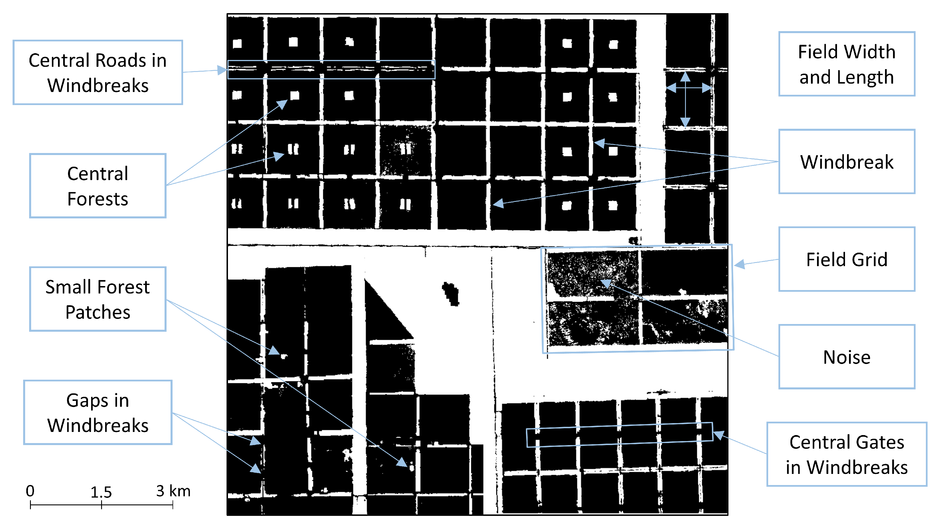Having the possibility to immediately compare the statistical distributions (Figure 7) of the artificial training set to the problematic features in the real-world data is one big advantage of using synthetically generated training data. Using manually labelled training data would require an additional step to derive statistics. A second benefit is that one can directly modify the features in the training data and, for instance, increase the maximum length of central forests. This would be almost impossible to realize with manually labelled data. Figure 6 shows the scene composition on which the synthetic images were based. Hence, the information where there are windbreaks, agricultural areas, and compact forests already exist, the extension of the prediction by these classes can easily be implemented by adding them to the class labels. Manual labelling of one additional class, e.g., to additionally classify pixels that belong to agricultural areas, would probably take weeks compared to the generation of a new synthetic data set which is easily feasible.

The visual analysis of the classification results also revealed that natural structures, for instance, water bodies, provoked falsely classified central forests and gaps. To prevent such misclassifications, we would have had to include more natural structures in the synthetic training data. Although we have shown through the integration of the small forest patches that it is possible to model naturally structured features, the synthetic design of such structures is more complex and time-intensive than the synthetic design of geometric features. In addition, this involves increased use of random variables and noise functions, which makes it difficult to numerically control the size or shape of the resulting landscape elements. Hence, there is always a trade-off between modelling the images as realistically as necessary while keeping the data generation process as simple and traceable as possible to make sure that the synthetic data design does not become more time-intensive than manual labelling. Additionally, we have also noticed that simply adding new features might harm the classification performance of existing features because statistical distributions that were suitable before may need to be adjusted as well.

In summary, the areas within the windbreak fractions were well identified as gaps such that the union of forest mask and detected gaps give a good approximation of where there should be forest to protect the fields from wind erosion. However, it must be considered that the detected gaps are spaces in the derived forest mask and not necessarily spaces in the actual windbreaks. Although the windbreak gaps are partly overestimated, the result can present a good overview of where there are hot spots of defective windbreaks and where the windbreaks are in good condition. Such maps can be particularly beneficial to Paraguayan forestry and environmental authorities such as the Instituto Forestal Nacional (INFONA), which is concerned with monitoring regulations such as the presence of windbreaks and central forests. It would, therefore, be interesting to investigate how the presented approach performs on higher resolved imagery from satellites, such as Planet (0.5–3 m) or WorldView (0.3–3.7 m) satellites. However, it is unclear whether these purely optical data can produce forest maps of comparable quality as the combination of the multispectral optical Sentinel-2 images with the radar images from Sentinel-1. In addition, Planet and WorldView data are less easily accessible. Another strength of synthetically generating data is that once a framework is set up, it can easily be adapted to related tasks or new application regions with a similar landscape. For instance, if the fields in a new application area have different shapes, are smaller, larger, or even round, the concerned features can be adapted in the data set generator, which is much faster than a setup from scratch. Additionally, the adaptation to new spatial image resolutions is possible, provided that the landscape features can still be adequately displayed on the specified image size (here, $1024\times 1024$ pixels). The Argentinian Chaco, extending across the country’s North, strongly resembles the Paraguayan Chaco and would therefore be another possible area where the presented method can be applied. Presumably, only small modifications of field sizes or barrier widths would be required. Bolivia, bordering Paraguay’s Northwest, also has large, agriculturally dominated regions. However, the fields there have thinner, but more frequent, windbreaks arranged in a striped rather than a grid pattern. Thus, more extensive adjustments to the data generator would probably be necessary. Another region where windbreaks between logged areas were left in a grid-like structure, almost identical to the structures in the Paraguayan Chaco, is the island Hokkaido in Japan [50]. Here, the forest strips are about 180 m wide and occur every 3 km, approximately.

It can be concluded that the presented approach works well for classifying features in binary images, which in return makes the gap and forest patch detection dependent on the quality of the binary mask. Therefore, it would be interesting to apply this method directly to RGB or even multispectral images in future research. However, the generation of artificial scenes with realistic surface textures can become a complex task. The fact that more complex tasks require a much larger number of training samples is not a problem since, theoretically, an infinite number of artificial training images can be generated, which is probably the greatest advantage compared with manual data generation. Most other studies using synthetic training data for remote sensing tasks address the detection of human-made objects such as aircraft [51,52,53], vehicles [54,55], or wind farms [28] and wind turbines [56]. Berkson et al., Liu et al., Weber et al., and Han et al. [51,53,54,55] use real satellite images and images generated with existing software and position the object of interest onto the satellite image background. Such an approach would not have been feasible for detecting central forests and windbreaks because these are not explicit objects such as aircraft. Similar to this study, Hoeser and Kuenzer [28], Hoeser et al. [56] and Isikdogan et al. [29] break away from the division into foreground and background and model the landscape scenes as a whole. Hoeser and Kuenzer [28] and Hoeser et al. [56] aim at a global detection of wind turbines in offshore wind farms and generate detailed and complex synthetic SAR-scenes of coastal areas to use these for training. Since complete landscape modelling is resource-expensive, we chose to pursue a more straightforward approach by focussing on a binary representation of the landscape. This proceeding is similar to that of Isikdogan et al. [29] who generated a synthetic data set to extract the centre lines of river networks in MNDWI images. Although river networks often have natural twists and turns, the authors successfully used straight geometries to model the river landscape. Thereby, they proved that it is not always necessary to generate synthetic images that perfectly imitate the real world, but that it might be sufficient to represent basic spatial contexts and features.

With our approach, we show that it is possible to model more complex landscapes, allowing analysis beyond a land cover classification. It is the first approach to synthetically model the spatial arrangement of different land use classes and subdivide the classes into further subclasses based on their geometry and arrangement. The methodology can be applied and adapted to new tasks and is straightforward to implement. Additionally, once a synthetic data set is created, and a model is set up and trained according to our approach, it is suitable to monitor the future developments of the considered landscape features on a regular basis. In Paraguay, there are no signs of the intensive use of land for cattle ranching and the accompanying deforestation diminishing in the coming years. Therefore, it is all the more important to ensure that at least the regulations implemented for the protection of soil, flora, and fauna are adhered to. Such supervision can be enabled through the presented method. The next step towards an operational system is to find the most suitable architecture for this task. A comprehensive comparison with different state-of-the-art architectures such as DeepLabV3+ will be an important challenge in subsequent research in order to obtain the best possible classification results.

6. Conclusions

This study presents a method to automatically detect natural landscape features relevant for environmental monitoring and conservation measures in Sentinel-1 and -2 images. In particular, we derived a forest mask and generated a synthetic training data set to classify gaps in windbreaks and small forest patches that are centrally located in agricultural areas in the Paraguayan Chaco. The customized U-Net, which was exclusively trained on synthetic data, reached F1 scores of 70.4% and 73.6% for the classification of windbreak gaps and central forests, respectively. The method we propose has the potential to be a great asset to the preservation of intact ecosystems because it enables the automated and exhaustive analysis of the current state of important landscape features.

References

1. Gill, E.; Da Ponte, E.; Insfrán, K.; González, L. Atlas of the Paraguayan Chaco; WWF (World Wildlife Fund); DLR (German Aerospace Center): Asunción, Paraguay, 2020; p. 98. [Google Scholar]
2. Da Ponte, E.; García-Calabrese, M.; Kriese, J.; Cabral, N.; Perez de Molas, L.; Alvarenga, M.; Caceres, A.; Gali, A.; García, V.; Morinigo, L.; et al. Understanding 34 Years of Forest Cover Dynamics across the Paraguayan Chaco: Characterizing Annual Changes and Forest Fragmentation Levels between 1987 and 2020. Forests 2022, 13, 25. [Google Scholar] [CrossRef]
3. La Republica del Paraguay. Decreto Nº 18831/86—Normas de Protección del Medio Ambiente. 1986. Available online: https://leap.unep.org/countries/py/national-legislation/decreto-no-1883186-normas-de-proteccion-del-medio-ambiente (accessed on 23 August 2022).
4. Institución Forestal Nacional. Resolución INFONA Nº 1242/2012. 2012. Available online: http://www.infona.gov.py/application/files/3614/2920/9237/2012_RESOLUCION_N_1242.pdf (accessed on 23 August 2022).
5. Institución Forestal Nacional. Resolución INFONA Nº 1001/2019. 2019. Available online: http://www.infona.gov.py/application/files/3015/7373/2886/RESOLUCION_INFONA_N_1001_2019.pdf (accessed on 23 August 2022).
6. Ministerio de Agricultura y Ganadería de la República del Paraguay. Resolución S.F.N. Nº 1105/2007. 2007. Available online: https://www.fepama.org/v1/RESOL%20SFN%20N%201105-07.pdf (accessed on 23 August 2022).
7. Ginzburg, R.; Torrella, S.; Adamoli, J. Las cortinas forestales de boque nativo, son eficaces para mitigar los efectos de la expansion agricola? Revista de la Asociacion Argentina de Ecologia de Paisajes 2012, 3, 34–42. [Google Scholar]
8. Borrelli, J.; Gregory, J.M.; Abtew, W. Wind Barriers: A Reevaluation of Height, Spacing, and Porosity. Trans. ASAE 1989, 32, 2023. [Google Scholar] [CrossRef]
9. Emrich, A.; Pokorny, B.; Sepp, C. The Significance of Secondary Forest Management for Development Policy; Deutsche Gesellschaft für Technische Zusammenarbeit (GTZ) GmbH: Eschborn, Germany, 2000. [Google Scholar]
10. Takle, E.S. Windbreaks and Shelterbelts. In Encyclopedia of Soils in the Environment; Hillel, D., Ed.; Elsevier: Oxford, UK, 2005; pp. 340–345. [Google Scholar] [CrossRef]
11. Liknes, G.C.; Meneguzzo, D.M.; Kellerman, T.A. Shape indexes for semi-automated detection of windbreaks in thematic tree cover maps from the central United States. Int. J. Appl. Earth Obs. Geoinf. 2017, 59, 167–174. [Google Scholar] [CrossRef]
12. Burke, M.W.; Rundquist, B.C.; Zheng, H. Detection of Shelterbelt Density Change Using Historic APFO and NAIP Aerial Imagery. Remote Sens. 2019, 11, 218. [Google Scholar] [CrossRef]
13. Ghimire, K.; Dulin, M.W.; Atchison, R.L.; Goodin, D.G.; Hutchinson, J.M.S. Identification of windbreaks in Kansas using object-based image analysis, GIS techniques and field survey. Agrofor. Syst. 2014, 88, 865–875. [Google Scholar] [CrossRef]
14. Piwowar, J.M.; Amichev, B.Y.; van Rees, K. The Saskatchewan Shelterbelt Inventory. Can. J. Soil Sci. 2016. [Google Scholar] [CrossRef]
15. Deng, R.X.; Li, Y.; Xu, X.L.; Wang, W.J.; Wei, Y.C. Remote estimation of shelterbelt width from SPOT5 imagery. Agrofor. Syst. 2016, 91, 161–172. [Google Scholar] [CrossRef]
16. Deng, R.X.; Li, Y.; Wang, W.J.; Zhang, S.W. Recognition of shelterbelt continuity using remote sensing and waveform recognition. Agrofor. Syst. 2013, 87, 827–834. [Google Scholar] [CrossRef]
17. Ahlswede, S.; Asam, S.; Röder, A. Hedgerow object detection in very high-resolution satellite images using convolutional neural networks. J. Appl. Remote Sens. 2021, 15, 018501. [Google Scholar] [CrossRef]
18. Zhu, X.X.; Tuia, D.; Mou, L.; Xia, G.; Zhang, L.; Xu, F.; Fraundorfer, F. Deep Learning in Remote Sensing: A Comprehensive Review and List of Resources. IEEE Geosci. Remote Sens. Mag. 2017, 5, 8–36. [Google Scholar] [CrossRef]
19. Ma, L.; Liu, Y.; Zhang, X.; Ye, Y.; Yin, G.; Johnson, B.A. Deep learning in remote sensing applications: A meta-analysis and review. ISPRS J. Photogramm. Remote Sens. 2019, 152, 166–177. [Google Scholar] [CrossRef]
20. Hoeser, T.; Kuenzer, C. Object Detection and Image Segmentation with Deep Learning on Earth Observation Data: A Review-Part I: Evolution and Recent Trends. Remote Sens. 2020, 12, 1667. [Google Scholar] [CrossRef]
21. Hoeser, T.; Bachofer, F.; Kuenzer, C. Object Detection and Image Segmentation with Deep Learning on Earth Observation Data: A Review—Part II: Applications. Remote Sens. 2020, 12, 3053. [Google Scholar] [CrossRef]
22. LeCun, Y.; Bengio, Y.; Hinton, G. Deep Learning. Nature 2015, 521, 436–444. [Google Scholar] [CrossRef] [PubMed]
23. Krizhevsky, A.; Sutskever, I.; Hinton, G.E. ImageNet Classification with Deep Convolutional Neural Networks. Commun. ACM 2017, 60, 84–90. [Google Scholar] [CrossRef]
24. Ronneberger, O.; Fischer, P.; Brox, T. U-Net: Convolutional Networks for Biomedical Image Segmentation. In Proceedings of the Medical Image Computing and Computer-Assisted Intervention—MICCAI 2015, Munich, Germany, 5–9 October 2015; Navab, N., Hornegger, J., Wells, W.M., Frangi, A.F., Eds.; Springer International Publishing: Cham, Switzerland, 2015; pp. 234–241. [Google Scholar]
25. Chen, L.C.; Papandreou, G.; Schroff, F.; Adam, H. Rethinking Atrous Convolution for Semantic Image Segmentation. arXiv 2017, arXiv:1706.05587. [Google Scholar]
26. Chen, L.C.; Zhu, Y.; Papandreou, G.; Schroff, F.; Adam, H. Encoder-Decoder with Atrous Separable Convolution for Semantic Image Segmentation. In Proceedings of the Computer Vision—ECCV 2018, Munich, Germany, 8–14 September 2018; Ferrari, V., Hebert, M., Sminchisescu, C., Weiss, Y., Eds.; Springer International Publishing: Cham, Switzerland, 2018; pp. 833–851. [Google Scholar]
27. Long, Y.; Xia, G.S.; Li, S.; Yang, W.; Yang, M.Y.; Zhu, X.X.; Zhang, L.; Li, D. On Creating Benchmark Dataset for Aerial Image Interpretation: Reviews, Guidances, and Million-AID. IEEE J. Sel. Top. Appl. Earth Obs. Remote Sens. 2021, 14, 4205–4230. [Google Scholar] [CrossRef]
28. Hoeser, T.; Kuenzer, C. SyntEO: Synthetic dataset generation for earth observation and deep learning—Demonstrated for offshore wind farm detection. ISPRS J. Photogramm. Remote Sens. 2022, 189, 163–184. [Google Scholar] [CrossRef]
29. Isikdogan, F.; Bovik, A.; Passalacqua, P. Learning a River Network Extractor Using an Adaptive Loss Function. IEEE Geosci. Remote Sens. Lett. 2018, 15, 813–817. [Google Scholar] [CrossRef]
30. Kong, F.; Huang, B.; Bradbury, K.; Malof, J. The Synthinel-1 dataset: A collection of high resolution synthetic overhead imagery for building segmentation. In Proceedings of the IEEE/CVF Winter Conference on Applications of Computer Vision, Snowmass Village, CO, USA, 1–5 March 2020; pp. 1814–1823. [Google Scholar]
31. He, B.; Li, X.; Huang, B.; Gu, E.; Guo, W.; Wu, L. UnityShip: A Large-Scale Synthetic Dataset for Ship Recognition in Aerial Images. Remote Sens. 2021, 13, 4999. [Google Scholar] [CrossRef]
32. Mereles, M.F.; Rodas, O. Assessment of rates of deforestation classes in the Paraguayan Chaco (Great South American Chaco) with comments on the vulnerability of forests fragments to climate change. Clim. Chang. 2014, 127, 55–71. [Google Scholar] [CrossRef]
33. Baumann, M.; Israel, C.; Piquer-Rodríguez, M.; Gavier-Pizarro, G.; Volante, J.N.; Kuemmerle, T. Deforestation and cattle expansion in the Paraguayan Chaco 1987–2012. Reg. Environ. Chang. 2017, 17, 1179–1191. [Google Scholar] [CrossRef]
34. Gorelick, N.; Hancher, M.; Dixon, M.; Ilyushchenko, S.; Thau, D.; Moore, R. Google Earth Engine: Planetary-scale geospatial analysis for everyone. Remote Sens. Environ. 2017, 202, 18–27. [Google Scholar] [CrossRef]
35. The European Space Agency. Sentinel-1 MSI/Cloud Masks. Available online: https://sentinel.esa.int/web/sentinel/technical-guides/sentinel-2-msi/level-1c/cloud-masks (accessed on 20 May 2022).
36. Google Developers. Eath Engine Data Catalog—Sentinel-2 MSI: MultiSpectral Instrument, Level-1C. Available online: https://developers.google.com/earth-engine/datasets/catalog/COPERNICUS_S2#bands (accessed on 4 July 2022).
37. Montero Loaiza, D. Awesome Spectral Indices. Available online: https://awesome-ee-spectral-indices.readthedocs.io/en/latest/index.html (accessed on 4 July 2022).
38. Kauth, R.; Thomas, G. The Tasselled-Cap—A Graphic Description of the Spectral-Temporal Development of Agricultural Crops as Seen by Landsat. In Proceedings of the Symposium on Machine Processing of Remotely Sensed Data, West Lafayette, IN, USA, 29 June–1 July 1976; pp. 41–51. [Google Scholar]
39. Harris, C.R.; Millman, K.J.; van der Walt, S.J.; Gommers, R.; Virtanen, P.; Cournapeau, D.; Wieser, E.; Taylor, J.; Berg, S.; Smith, N.J.; et al. Array programming with NumPy. Nature 2020, 585, 357–362. [Google Scholar] [CrossRef]
40. van der Walt, S.; Schönberger, J.L.; Nunez-Iglesias, J.; Boulogne, F.; Warner, J.D.; Yager, N.; Gouillart, E.; Yu, T. Scikit-image: Image processing in Python. PeerJ 2014, 2, e453. [Google Scholar] [CrossRef]
41. Spencer, K.; Imas, A. OpenSimplex Noise. Available online: https://github.com/lmas/opensimplex (accessed on 3 November 2021).
42. Bradski, G. The OpenCV Library. Dr. Dobb’s J. Softw. Tools Prof. Program. 2000, 25, 120–123. [Google Scholar]
43. He, K.; Zhang, X.; Ren, S.; Sun, J. Deep Residual Learning for Image Recognition. In Proceedings of the 2016 IEEE Conference on Computer Vision and Pattern Recognition (CVPR), Las Vegas, NV, USA, 27–30 June 2016; pp. 770–778. [Google Scholar] [CrossRef]
44. Chen, L.C.; Papandreou, G.; Kokkinos, I.; Murphy, K.; Yuille, A.L. DeepLab: Semantic Image Segmentation with Deep Convolutional Nets, Atrous Convolution, and Fully Connected CRFs. IEEE Trans. Pattern Anal. Mach. Intell. 2016, 40, 834–848. [Google Scholar] [CrossRef]
45. Abadi, M.; Agarwal, A.; Barham, P.; Brevdo, E.; Chen, Z.; Citro, C.; Corrado, G.S.; Davis, A.; Dean, J.; Devin, M.; et al. TensorFlow: Large-Scale Machine Learning on Heterogeneous Systems. Available online: https://www.tensorflow.org/ (accessed on 7 January 2022).
46. Chollet, F.E.A. Keras. Available online: https://keras.io (accessed on 7 January 2022).
47. Kingma, D.P.; Ba, J. Adam: A Method for Stochastic Optimization. arXiv 2014, arXiv:1412.6980. [Google Scholar] [CrossRef]
48. Cohen, J. A Coefficient of Agreement for Nominal Scales. Educ. Psychol. Meas. 1960, 20, 37–46. [Google Scholar] [CrossRef]
49. Padilla, R.; Passos, W.L.; Dias, T.L.B.; Netto, S.L.; da Silva, E.A.B. A Comparative Analysis of Object Detection Metrics with a Companion Open-Source Toolkit. Electronics 2021, 10, 279. [Google Scholar] [CrossRef]
50. Voiland, A. A Windbreak Grid in Hokkaido. Available online: https://earthobservatory.nasa.gov/images/146664/a-windbreak-grid-in-hokkaido (accessed on 1 April 2022).
51. Berkson, E.E.; VanCor, J.D.; Esposito, S.; Chern, G.; Pritt, M. Synthetic Data Generation to Mitigate the Low/No-Shot Problem in Machine Learning. In Proceedings of the 2019 IEEE Applied Imagery Pattern Recognition Workshop (AIPR), Washington, DC, USA, 15–17 October 2019; pp. 1–7. [Google Scholar] [CrossRef]
52. Shermeyer, J.; Hossler, T.; Van Etten, A.; Hogan, D.; Lewis, R.; Kim, D. RarePlanes: Synthetic Data Takes Flight. In Proceedings of the IEEE/CVF Winter Conference on Applications of Computer Vision (WACV), Waikoloa, HI, USA, 3–8 January 2021; pp. 207–217. [Google Scholar]
53. Liu, W.; Luo, B.; Liu, J. Synthetic Data Augmentation Using Multiscale Attention CycleGAN for Aircraft Detection in Remote Sensing Images. IEEE Geosci. Remote Sens. Lett. 2022, 19, 1–5. [Google Scholar] [CrossRef]
54. Weber, I.; Bongartz, J.; Roscher, R. Artificial and beneficial—Exploiting artificial images for aerial vehicle detection. ISPRS J. Photogramm. Remote Sens. 2021, 175, 158–170. [Google Scholar] [CrossRef]
55. Han, S.; Fafard, A.; Kerekes, J.; Gartley, M.; Ientilucci, E.; Savakis, A.; Law, C.; Parhan, J.; Turek, M.; Fieldhouse, K.; et al. Efficient generation of image chips for training deep learning algorithms. In Proceedings of the SPIE, Automatic Target Recognition XXVII, Anaheim, CA, USA, 10–11 April 2017; Sadjadi, F.A., Mahalanobis, A., Eds.; SPIE: Bellingham, WA, USA, 2017. [Google Scholar] [CrossRef]
56. Hoeser, T.; Feuerstein, S.; Kuenzer, C. DeepOWT: A global offshore wind turbine data set derived with deep learning from Sentinel-1 data. Earth Syst. Sci. Data Discuss. 2022, 2022, 1–26. [Google Scholar] [CrossRef]
Figure 1. Overview of the Paraguayan Chaco (right map) showing regular grids of cropland and cattle areas, which are separated by windbreaks and partly contain central forest patches (magnifications (a and b)). Background: Sentinel-2 RGB-image—median of 10/2020–12/2020.
Remotesensing 14 04327 g001
Figure 2. Overview of major building blocks of the data processing workflow.
Remotesensing 14 04327 g002
Figure 3. Workflow for the classification of central forest patches and gaps in windbreaks in the Paraguayan Chaco based on synthetic training data. The boxes with a double rim denote data products or intermediate results and the boxes with normal rim are actions.
Remotesensing 14 04327 g003
Figure 4. Binary forest—non-forest mask of the Paraguayan Chaco as derived from Sentinel-1 and Sentinel-2 time series for the year 2020. The magnifications a and b show the spatial structure of the forest landscape in detail.
Remotesensing 14 04327 g004
Figure 5. Example tile from the binary forest mask of the Paraguayan Chaco that shows all features which were considered during the generation of the synthetic data set. White areas represent forest and black areas represent non-forest areas.
Remotesensing 14 04327 g005
Figure 6. Examples of synthetically generated scenes with their corresponding class labels and a scene composition revealing the landscape features of which the scenes are composed. Areas that appear grey in the second row are actually noisy areas with forest and non-forest pixels.
Remotesensing 14 04327 g006
Figure 7. Histograms of the synthetically generated training set (8000 samples). Every image contains ten field grids with different features. Note that the validation set (2000 samples) histograms look almost identical, and are therefore not displayed. Since all samples were generated on a random basis, the split of the data into training and validation set corresponds to a random sampling.
Remotesensing 14 04327 g007
Figure 8. Structure of the used U-Net with ASPP module.
Remotesensing 14 04327 g008
Figure 9. Classification results for the forest mask (RF classifier) and the classified windbreak gaps and central forests (CNN). Two tiles (A and B) with magnifications (a and b) of the agricultural areas.
Remotesensing 14 04327 g009
Figure 10. Classification results for the forest mask (RF classifier) and the classified windbreak gaps and central forests (CNN). Tiles (A–G).
Remotesensing 14 04327 g010