Water Level Change Monitoring Based on a New Denoising Algorithm Using Data from Landsat and ICESat-2: A Case Study of Miyun Reservoir in Beijing

Abstract

Inland lakes or reservoirs are the main surface water resources, related to people’s survival and social development. On-site water level data are critical for water resource management, while satellite laser and remote sensing data are a significant tool for long-term change monitoring. In this study, we took the Miyun Reservoir, the most important source of drinking water in Beijing, as the research area. We used Landsat images and the Ice, Cloud, and Land Elevation Satellite (ICESat-2) for small-scale water level change monitoring and inversion across unrecorded periods. First, we proposed a new two-step denoising method based on local statistics to denoise the ATL03 single photon data from 2018 to 2020, and extracted the effective elevation information of Miyun Reservoir. Second, based on Landsat images from 1984 to 2020, the MNDWI index was used to extract the water area and generated a percentage map of water occurrence. Finally, the water and land boundary elevation were selected from the effective photon elevation information according to the boundary position under each percentage of the water generation percentage graph, the area, and the water level elevation model (A–E model) was established, and the water level values of unrecorded periods were inverted. The denoising results showed that the denoising accuracy of all data is higher than 95%. The area of Miyun Reservoir has changed greatly in the past 37 years, especially in the northeast corner and northern region. The inverted water level elevation had a strong correlation with the measured value, the correlation coefficient reached 0.97, the root mean square error (RMSE) was 0.553 m, and the estimated water level value was highly consistent with the recorded value and fluctuated dramatically from 1984 to 2020. This method complements the traditional water level mapping method, provides a new idea for the monitoring of water level changes in lakes or reservoirs without field records, and also contributes to the timely and effective monitoring and management of global lake and reservoir water level and time changes.

1. Introduction

Only roughly 2.5% of the globe is covered by fresh water, and less than 1% of fresh water resources occurs on the surface, with only 0.007% of that available for human use [1,2]. The average per capita water availability in China is less than one-fourth of the global average, and China is one of the 13 countries with the fewest water resources in the world, and the available water distribution is unequal, with a major concentration of freshwater resources in the south [3,4]. Reservoirs are an important surface water source, which is an artificial lake formed by building a dam along a flowing river. Unlike lakes formed by natural processes, reservoirs are created by humans to provide water and hydroelectricity for our own requirements, and they are highly related to human activities [5]. Therefore, it is critical to monitor the changes in the water level and area of lake and reservoirs. However, it is difficult to measure the area and depth of lakes and reservoirs directly.

Traditional water level monitoring of lake or reservoirs mostly relies on hydrological stations, shipborne sonar instruments, single- or multi-beam echo sounders, or airborne sounders to obtain water depth maps. These types of methods often consume considerable manpower and material resources, and the cost is very high [6,7]. With the rapid development of deep space exploration and remote sensing technology, real-time, macroscopic, multi-temporal, multi-spectral, dynamic, and repeated surface information can be generated [8]. An increasing number of scholars have applied satellite remote sensing technology in continuous change monitoring of lake reservoirs.

At present, many countries and international organizations have deployed short-revisit period altimetry satellites to carry out dynamic monitoring of important global water bodies, such as the Global Reservoirs/Lakes platform established by the United States Department of Agriculture [9,10], Hydroweb established by the Laboratory of Space Geophysical and Oceanographic Studies in France in 2011 [11], the River and Lake project of the European Space Agency (ESA) [12], and the Database for Hydrological Time Series of Inland Waters (DAHITI) constructed by the German Institute of Geology in 2013 [13]. In addition, many scholars have combined remote sensing images and altimetry data to realize dynamic monitoring of the water level and area of lake reservoirs. For example, Geoscience Laser Altimeter System (GLAS) and Landsat images were adopted to build an area-water level model, monitor lake changes, reconstruct time series of lake water level data, and estimate fluctuations in lake and reservoir water volume [6]. Ma et al. [14] employed Multiple Altimeter Beam Experimental Lidar (MABEL) and Landsat TM data to estimate the water level and storage capacity of Lake Mead in the United States during the period from 1987 to 2007. Li et al. [15] considered the water occurrence percentage instead of specific isolines to obtain lake elevation information by correlating altimetry data retrieved from airborne lidar instruments. Numerous research results have been obtained on dynamic change monitoring of the water level based on the combination of satellite altimetry data and remote sensing images. However, most current studies are based on large lake reservoirs. In terms of lake reservoirs with small areas, due to the large diameter of radar altimetry satellite footprints, the echo signal easily experiences interference from the surrounding terrain. Although existing laser height measurement data exhibit a sufficiently small footprint, the distance between satellite orbits is relatively large, which is likely to result in missing data with regard to smaller lake reservoirs.

Based on the above problems, due to the multi-beam laser and single-photon laser detection capabilities, the Ice, Cloud and land Elevation Satellite (ICESat-2) can cover a large number of photon echo signals, and its laser achieves a strong penetrability of water bodies. It offers dense and accurate measurements, and has been widely used in the study of water level changes in inland lakes [15,16,17,18,19]. ICESat-2 photon data partially overlap the water surface, which can be considered to measure the lake water level and extract surface waves in oceans, while the remainder of ICESat-2 photons penetrates the water surface and reaches the bottom water layer [20]. Zhang et al. [21] constructed a surface area regression model for lakes to establish the water level sequence of lakes based on water level elevation data obtained by the ICESat and area data obtained by the Moderate Resolution Imaging Spectroradiometer (MODIS) on the same date. To accomplish water depth inversion, Armon et al. [19] obtained high-resolution water occurrence data and utilized the effective ICESat-2 elevation data to perform linear fitting with varying water occurrence percentages.

However, because the ICESat-2 system transmits and receives weak signal photons, background disturbances such as solar background noise, system dark noise, and atmospheric scattering noise have a significant impact [22]. The most controversial and challenging aspect of ICESat-2’s data processing is how to successfully eliminate noisy photons. Numerous specialists and academics have suggested a number of processing algorithms [23] based on the characteristics that the orbits of ICESat-2 are spread in a narrow band. Algorithms based on image processing [24,25], algorithms based on local statistics [26,27], and algorithms based on density clustering [28,29,30] are three groups into which denoising algorithms now in use may be categorized. In some areas, these algorithms have shown positive outcomes. Although the image processing-based denoising method may eliminate noise to a certain extent, some information will be lost during the conversion of data into images, making it challenging to identify targets; the decision of the threshold, which is challenging to adjust to photon point clouds in various contexts, determines the denoising impact of algorithms based on local statistical factors. The denoising method based on density clustering depends on the density difference between the signal and noise point clouds; however, under a strong background and complicated terrain circumstances, it is challenging to obtain high accuracy.

In order to give better play to the practical application of push scan lidar and make up for the problems of the above algorithms, this study proposes a new two-step local statistical denoising method. The adaptive threshold is obtained by calculating the mean value of the square of the K-neighborhood distance of each photon, and finally the denoising processing of the complete detection data is realized.

The main purpose of the study was to dynamically detect the water level of Miyun Reservoir and invert the water level information of unrecorded years. To begin, we proposed a new two-step denoising method based on statistical histograms, in view of the problem of a large amount of background noise in ATLAS laser data. Then, an area and water level elevation model (A–E model) was developed using denoised single-photon data and water extraction results from Landsat images, and the known reservoir area was utilized to invert the water level elevation under different time periods. Finally, by analyzing the related causes of water level changes from the natural and human perspectives, it provides a scientific basis for water resources and ecological protection in the basin. This study has references for water level estimation and inversion of small lakes and reservoirs such as Miyun Reservoir. On the other hand, it has analytical significance for future global climate change and ecological assessment.

2. Materials and Methods

2.1. Study Area

Miyun Reservoir is located in the northeast of Beijing, China, in the center of Miyun District. It is the largest reservoir in North China and the major water source in the capital, and its main functions include flood control and water supply. The average annual temperature of the basin is 10.9 °C, the main rainfall is concentrated from June to September, and the annual average rainfall is 480 mm [31]. The reservoir has a large surface area of 188 km² and a total storage capacity of 437.5 GL, as well as a complicated bathymetry characterized as a mountain valley reservoir type [32]. Due to the dual influences of environmental factors including the climate environment, precipitation, water evaporation, and human intervention, such as the South-to-North Water Diversion Project, the Miyun Reservoir experiences changes in the degree of incomplete regularity.

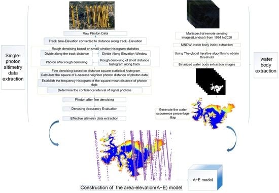
Figure 1 illustrates the workflow of this study. Based on the new denoising algorithm, we denoises the ICESat-2 single-photon data to extract effective photons and obtain elevation information (Section 2.3). Then, we used the effective elevation data combined with the water area extracted from the time-series Landsat images to establish a water occurrence percentage map (Section 2.4). The area-elevation model of Miyun Reservoir is established by producing different contours of water occurrence percentage, and the water level information of the reservoir in other periods was obtained by inversion (Section 2.5). Furthermore, the inversion accuracy is evaluated by the measured water level information (Section 3.3). Finally, the driving factors of the interannual variation of Miyun Reservoir are analyzed (Section 4).

2.2. Datasets

2.2.1. Photon Data

ICESat-2 is the earth’s first laser altimetry satellite using single-photon technology from NASA, which is equipped with the Advanced Topographic Laser Altimeter System (ATLAS) [33]. ATLAS has 6 laser beams with a footprint spacing of only 0.7 m, which can achieve continuous detection of 6 bands (https://nsidc.org/data/icesat-2/ (accessed on 5 April 2019)). The ATL03 (Global Geolocation Data) product (https://search.earthdata.nasa.gov/search (accessed on 5 April 2019)) is one of the main second-level products and constitutes important basic data for the generation of advanced products. The experiments in this study used ICESat2/ATLAS data from 2018 to 2020, and the vertical lake information was extracted using ATL03 data that were taken from the secondary product, and 32 beams and 9 tracks worth of data were collected. Using the vector map of the administrative boundaries, a cropped image of the Miyun area was generated, and the subsatellite data were shown in Figure 2.

2.2.2. Landsat Imagery

In this study, we collected Landsat 5 TM, Landsat 7 ETM+, and Landsat 8 OLI surface reflectance imagery datasets covering the Miyun Reservoir study area from August 1984 to December 2020 from the USGS website (https://earthexplorer.usgs.gov (accessed on 24 October 2020)) and geospatial Data Cloud (http://www.gscloud.cn/search (accessed on 24 October 2020)). Through the combination of visual interpretation and cloud content filtering, we selected a total of 320 L1TP level valid data above the study area where the visual effect does not contain ice and snow, and the image cloud content is less than 10%. Figure 3 shows a histogram of available Landsat imagery screened during 1984–2020. A total of 320 Landsat images were used to extract the water boundaries and calculate the area of Miyun Reservoir from 1984–2020, and were used for inversion of water level elevations.

2.2.3. Measured Water Level Data

The field observations used in this study were acquired from daily data pertaining to the Beijing Water Regime of Large- and Medium-Sized Reservoirs (http://nsbd.swj.beijing.gov.cn/dzxsksq.html (accessed on 24 October 2020)) released by the Beijing Municipal Water Affairs Bureau. We have collected daily monitoring data on reservoir water levels from 30 October 2009 to 10 January 2021, compared the measured water level data with the prediction data of A–E model, and conducted correlation analysis to verify the water level inversion results (see Section 3.3.1 and Section 3.3.2). We sorted the data according to the time series, as shown in Figure 4. From 2009 to 2013, the water level of Miyun Reservoir was relatively stable, at about 136 m; from 2014 to 2015, it fell sharply to 133 m, from October 2015 to October 2019, and the water level has been rising to 150 m, a change of about 17 m, and fluctuating around 149 m from 2019 to 2020.

2.3. Single-Photon Altimetry Data Denoising Algorithm

We proposed a new two-step (rough step and fine step) denoising algorithm. Firstly, spaceborne single-photon data contain three-dimensional geographic information, and single-beam photon data are distributed as strips of point clouds along the flight direction. Therefore, in actual photon denoising, three-dimensional geographic coordinate-based photon data were converted into two-dimensional distance-elevation along-orbit data via dimension reduction. Then, the rough denoising step based on a small-window statistical histogram and fine denoising step based on a distance square statistical histogram were conducted. The process of denoising method is shown in Figure 5.

2.3.1. Rough Denoising Based on a Small-Window Statistical Histogram along the Track

The effective signal and noise photon densities returned from the ground surface are highly different between the horizontal and vertical directions. In this paper, considering terrain fluctuations and other factors, a rough denoising method based on a local small-window histogram is proposed, which divides the target data into several small windows according to the distance and elevation along the orbit and counts photon data in each small window to achieve rough denoising. First, the target data are divided into N along-orbit distance windows according to a fixed window D_{along_track}, and the single along-orbit distance window is then divided into M elevation sub-windows according to the elevation window D_{elevation_dir}. The relationship between the elevation window and the track window is as follows:

$$D_{elevation\_dir}=D_{along\_track}·\tan 2\alpha$$

(1)

In Equation (1), α is the rough terrain slope in the along-track window; the along-track distance window is determined by the terrain slope, which can be reduced with the increase of the slope, and is usually set to 10–100 m.

Subsequently, the number of photons in each elevation sub-window within a single local window along the track is counted, and an elevation-photon number histogram is constructed. The three-histogram statistic with the highest frequency among the constructed histograms is extracted. The photon data in the upper program sub-window with the highest frequency in the default histogram provide effective signal data. According to Equation (2), it is determined whether the other two frequencies corresponding to the photon data of the elevation window indicate effective signals. The default photon data in the elevation sub-window with the highest frequency in the histogram are valid signals, and according to Equation (2), it is ascertained whether the photon data in the elevation window corresponding to the other two frequencies are valid signals:

$$signal\_photon=\left\{\begin{array}{ll}S\_N1,& N2<{\sigma }_{1}N1\\ S\_N1+S\_N2,& N2\ge {\sigma }_{1}N1\&N3<{\sigma }_{2}N1\\ S\_N1+S\_N2+S\_N3,& N3\ge {\sigma }_{2}N1 \end{array}\right.$$

(2)

where $signal\_photon$ denotes the effective signal photon data in a single orbit window, N1, N2, and N3 and S_N1, S_N2, and S_N3 denote the photon data in the corresponding elevation intervals of the highest three frequencies (N1 ≥ N2 ≥ N3) in the orbit window, and both ${\sigma }_1$ and ${\sigma }_2$ are empirical values.

2.3.2. Fine Denoising Based on a Distance Square Statistical Histogram

After rough denoising, there remains only a small amount of noise in the photon data, and the distance between the remaining effective signal photons is smaller than that between the effective signal photons and noise photons or that between the noise photons. To effectively distinguish noise photons, we calculated the mean value of the square of the K-neighborhood distance of each photon based on Equation (3):

$$Dist\_av{e}_K(i)=\frac{1}{K}{\displaystyle \sum _{i\in N_K(i)}({(x_i-x_j)}^2+{(h_i-h_j)}^2)};i\in D$$

(3)

In the above equation, i denotes each photon object in the remaining photon data set D after rough denoising, $Dist\_av{e}_K(i)$ is the mean value of the square of the photon distance between the i point and its K neighbours, $x_i$ and $x_j$ are the distances along the tracks of photons i and j, respectively, and $h_i$ and $h_j$ are the heights of photons i and j, respectively.

Subsequently, a K-neighborhood distance squared frequency histogram was generated. This histogram approximates a one-sided normal distribution and therefore exhibits normal distribution characteristics. A confidence interval of $1\times \sigma$ was adopted as the demarcation point between the signal and noise photons. In actual engineering, we used a multi-parallel mechanism to enhance the efficiency of denoising. The photons were divided into M segments, and each segment’s distance histogram is calculated, and the effective photons are extracted (M is 1000, σ is 0.6826).

2.3.3. Precision Analysis Based on Statistical Indicators

Referring to the remote sensing image classification accuracy evaluation method, this paper employs a confusion matrix and statistical indicators to analyze the single photon denoising accuracy, mainly by comparing each photon attribute after classification to the real photon attribute to obtain denoising results. The calculation equation is as follows:

$$AC=\frac{TP+TN}{TP+FP+TN+FN}$$

(4)

where AC is the denoising accuracy, TP is the total number of effective signal photons correctly classified by the algorithm, TN is the total number of noise photons correctly classified by the algorithm, FN is the total number of effective signal photons incorrectly classified as noise photons by the algorithm; and FP is the total number of noise photons incorrectly classified as effective signal photons by the algorithm.

In addition, four statistical indicators are determined to evaluate the denoising accuracy [23]. The calculation equations for the four indicators of kappa coefficient K, the recall rate R, accuracy P, and comprehensive evaluation index F are as follows:

$$K=\frac{P_0-P_e}{1-p_e};R=\frac{TP}{TP+FN}; P=\frac{TP}{TP+FP}; F=\frac{2PR}{P+R}$$

(5)

2.4. Water Extraction Based on Landsat Images

In our study, the extraction results of multi-spectral remote sensing images are combined with single-photon laser data to obtain long-term changes in lake and reservoir water level and elevation.

Therefore, we used the MNDWI index to extract the water of Miyun Reservoir from 1984 to 2020. MNDWI (modified normalized difference water index) is sensitive to bare surface water and is one of the most widely used and stable water identification indexes. Studies have demonstrated the advantages of using MNDWI to extract water [34,35,36]. First, the green and shortwave infrared band information contained in the remote sensing images is extracted with a MATLAB function, and a single-band image is then obtained with the formula below:

$$\mathit{MNDWI}=\left(\mathit{Green}-\mathit{SWIR}1\right)/\left(\mathit{Green}+\mathit{SWIR}1\right)$$

(6)

SWIR1 denotes the shortwave infrared frequency band (Landsat TM and Landsat ETM+ data frequency band 5 or Landsat 8 OLI data frequency band 6), and Green denotes the green band (Landsat TM and Landsat ETM+ data frequency band 2 or Landsat 8 OLI data frequency band 3). After water index calculation, a single-band image is obtained, and an appropriate threshold value must be set to realize image segmentation and generate a binarized image with the water as the foreground.

Due to the characteristics of maximizing the contrast between the target water and background area after water index calculation, instead of using the set threshold, we used the global iterative algorithm to automatically select the optimal threshold and generate binarized images [37].

Therefore, we calculated the MNDWI value of the selected Landsat images from 1984 to 2020, then used the global iterative algorithm to determine the segmentation threshold and extract the water body, resulting in the segmented binarized images. Second, we used the MATLAB function “bwareaopen” to process the binarized image and eliminate tiny water and noise.

2.5. Construction of the Area-Elevation (A–E) Model

The purpose of this study was to obtain long-term changes in water levels and elevations in lakes and reservoirs. Therefore, we used the photon data after denoising and the water extraction results of Landsat images to establish a model of the surface area and water level elevation of the lake reservoir to invert the long-term change of the water level of the lake reservoir. The extraction flowchart is shown in Figure 6.

After processing the multiple binarized images, we chose the map with the largest water area in the binarized images and extracted the boundary as the maximum extraction boundary, followed by mask extraction. We overlaid and normalized the binarization result after mask extraction to determine the percentage of water in each pixel within the maximum mask area and generate the water percentage occurrence map as follows:

$$I\_DJ(\mathrm{i}, \mathrm{j})={\displaystyle \sum _{k=1}^{n}I{0}_k(\mathrm{i},\mathrm{j})}/n$$

(7)

In the formula, $I\_DJ(\mathrm{i}, \mathrm{j})$ represents the percentage of water occurrence in the i-th row and j-th column of the superimposed image, $\mathrm{I}{0}_{\mathrm{k}}(\mathrm{i},\mathrm{j})$ represents the value of the i-th row and the j-th column of the k-th binary image, and n represents the number of binarized images.

We defined the contour lines enclosed by the same percentage value as equal percentage lines based on the water occurrence percentage map, and calculated the area enclosed by different equal percentage lines as the area of the water occurrence percentage map, and according to the spatial resolution of the image. Finally, the actual area represented by the various equal percentage lines was determined, which was used as the area element in the A–E model construction. Formula 8 shows the area under each equal percentage line:

$$area={\displaystyle \sum _{\mathrm{m}=1}^N{\displaystyle \sum _{k=1}^{M}ob{j}_{(m,k)}}\times rati{o}^{{}_2}}$$

(8)

In the formula, N and M represent the width and height of the binarized image, respectively; $ob{j}_{(m,k)}$ indicates that the judgment pixel is within the range enclosed by the equal percentage line, if it is, it is expressed as 1; $ratio$ indicates the spatial resolution corresponding to the image.

3. Results

We show the effects of the new two-step denoising algorithm in Section 3.1. We explain how to create the water occurrence percentage map in Section 3.2 and describe how to construct and select the AE model in Section 3.3.

3.1. Denoising Based on the Two-Step Method of the Statistical Histogram

Choosing data at 10:00 a.m. in Beijing on 8 October 2019, as an example, after latitude and longitude screening, the original photon data along the track distance (ATD) are shown in the blue part of Figure 7a. The ATL03 data are approximately 800 m away from the gate width. The small-window statistical histogram method in Section 2.3.1 performed rough photon denoising, and the results of rough denoising are shown in the red part of Figure 7a,b. Subsequently, the fine denoising method in Section 2.3.2 was applied to finely denoise the rough denoising results. Moreover, to increase the operation speed and achieve operation time savings, in fine denoising, the data were extracted in sections according to 1000 photons along the track, and the extraction results are shown in Figure 7c. Figure 7d shows NASA’s extracted results; the data obtained with the algorithm in our study mostly contain photons at confidence levels 3 and 4, and more effective signal photons are extracted.

Because background noise in nighttime data (such as solar background noise, system Dark noise, and atmospheric scattering noise) is less than in the daylight data, the matching photon data will have less noise. To further boost denoising efficiency, we used the fine denoising phase of our proposed two-step denoising method for denoising processing for nighttime data. Figure 8 shows data obtained in the early morning of 7 October 2020, Beijing time, after only fine denoising process. The contrast in Figure 8 shows that, in the case of less photon noise, we can only apply the fine denoising section to achieve acceptable results and further enhance the denoising efficiency. The performance described above also shows the availability of our new two-step denoising algorithm.

The confidence that a single photon is correctly classified as a feature type is stored in the ATL03 data set (/gt*/heights/signal_conf_ph). In this paper, photons at confidence levels 3 and 4 and photons obtained through visual interpretation are considered true values. Accuracy evaluation is performed by calculating the confusion matrix. The results are provided in the tables below, where

Table 1. Confusion matrix and daytime data precision analysis results.

	This Paper	Effective Signal Photons	Noise Photons	Total	0.9751 (AC)
True Value					0.8783 (K)
Effective signal photons		256,744 (TP)	7271 (FP)	264,015	0.9725 (P)
Noise photons		184 (FN)	35,038 (TN)	35,222	0.9993 (R)
Total		256,928	42,309	299,237	0.9857 (F)

lists the daytime data accuracy analysis results, and

Table 2. Confusion matrix and nighttime data precision analysis results.

	This Paper	Effective Signal Photons	Noise Photons	Total	0.9955 (AC)
True Value					0.9762 (K)
Effective signal photons		14,046 (TP)	20 (FP)	14,066	0.9986 (P)
Noise photons		35 (FN)	411 (TN)	446	0.9975 (R)
Total		14081	431	14,512	0.9980 (F)

summarizes the nighttime data accuracy analysis results. These tables show that the accuracy of denoising results in daytime data and nighttime data are 97.51% and 99.55%, respectively. According to statistics, the denoising accuracy of all data is higher than 95%. Based on the above four statistical indicators, the results are good, and the nighttime data processing results are better than the daytime data processing results because nighttime data contain less sun-induced background noise. Based on the statistical results, on the one hand, it has the potential to improve the efficiency of denoising; on the other hand, based on NASA’s denoising results, our denoising results are equally good.

3.2. Extracting Reservoir Area of Time Series and Water Occurrence Percentage Map

We extracted the water Binary maps of Miyun Reservoir from Landsat images using the proposed water extraction method, extracted the binary image’s boundaries and converted it to a vector, and assessed the accuracy of the water extraction results through visual interpretation. The ATM5 image on 21 September 1991 and Landsat 8 OLI image on 18 September 2019 were chosen as examples (the original images are displayed in three bands, i.e., the near-infrared, red, and green bands). As shown in Figure 9 and Figure 10, the method proposed in this paper achieved a satisfactory water boundary extraction effect.

We selected a total of 320 cloud-free images from 1984 to 2020, and calculated and binarized the water body index for all cloud-free images, setting the foreground water pixels to 1 and the background non-water pixels to 0. We superimposed the binarized value maps of all image processing and normalize them to generate a water occurrence map, as shown in Figure 11. The water occurrence percentage gradually decreases from blue to yellow to red. Blue indicates locations where the water occurrence percentage is 1, i.e., the pixel has remained water for many years, and red indicates locations where the water occurrence percentage is close to 0.1. The figure also shows that Miyun Reservoir has changed considerably over the past 40 years, especially in the northeast corner and northern area. The northwest corner is the entrance of the Baihe water system of Miyun Reservoir, and the northeast corner is the entrance of the Chaohe water system.

3.3. Inversion of Water Level Elevation

3.3.1. Construction and Selection of the A–E Model

Before matching the water level and area of the lake and reservoir, the photon data were manually edited, including deleting photons located at the center of the lake and reservoir while retaining photons located at the water–land junction of the reservoir, we extracted and averaged the photon elevation at each equal percentage line, using the elevation information at each isobath as the water level elevation in the A–E model. As a result, we developed a one-to-one relationship between water level elevation and water occurrence percentage area.

Different regression analysis models are compared in this study in order to develop a better A–E model. The independent variable is the water occurrence percentage area, and the dependent variable is the corresponding water level height. Substitute variables in various regression models, including the comparative linear model, one-dimensional quadratic polynomial model, logarithmic model, exponential model, etc., and fit the linear model. Create distinct A–E models by determining several regression equations. Then, multiple regression equations were developed in order to establish different A–E models. Using the observed water level elevations of existing years, we evaluate the coefficient of determination R² of the inversion of water level elevations. Finally, we evaluate the inversion accuracy of the multi-year change trend of the lake and reservoir, including the change of area and water level.

As indicated in

Table 3. Different regression models and coefficients of determination.

Regression Model	Coefficient of Determination (R2)
Linear regression model	0.9748
Quadratic polynomial model in one variable	0.9802
Logarithmic regression model	0.9747
Exponential regression model	0.9733

, the coefficients of determination of the linear regression and logarithmic regression models are similar, the coefficient of determination of the exponential regression model is the lowest, and the coefficient of determination of the univariate quadratic polynomial is the highest. The relationship between the water area and elevation was thus established. The fitting function of $y=-0.0006\times x^2+0.3341\times x+106.07$ was obtained, with R² = 0.9802, and shown in Figure 12.

The corresponding water level was calculated with the obtained regression model based on the images from 2009 to 2020 and the area of each cloud-free image, and the result was compared to the measured daily water level.

The coefficient of determination (R²) between the inverted and measured water levels was computed to express the accuracy of water level inversion, and the R² reached 0.9702, which reflects a strong correlation, as is shown in Figure 13a,b. Among the results, there were obvious error points on 28 January 2010, 13 February 2010, 17 March 2010, 10 January 2012, and 13 February 2013. After analysis of these images and boundary extraction settings, snow and ice conditions were detected in the images, and the ice conditions differed across various regions. Therefore, although the image extraction boundary was highly consistent with the original image boundary, the extracted area was affected by a certain error due to ice and snow in the images, which resulted in a significant difference in the water level elevation inversion performance. For example, affected by ice, snow, and thin clouds on 21 January 2019, as shown in Figure 14, there occurred thin ice near the shore of the reservoir, and the area at the center, such as the area marked with a black frame, was not frozen. Therefore, this part was not recognized as a water body. This led to inaccurate area recognition, which resulted in errors in the obtained water level elevation values. Excluding any obviously incorrect water level values, the R² between the inverted and measured water level values reached 0.9829.

The above analysis results show that there was a correlation between the inversion water level and the real water level, but the water level value still had a certain absolute inaccuracy. We thought that the gap between the ICEsat-2 reference water level and the measured reference water level in Miyun Reservoir may cause the elevation difference. To further evaluate the accuracy of the water level inversion based on the Dagu Elevation Datum of the measured water level, we undertook an elevation datum transformation and removed individual error points for the inverted water level. After correction for the inverted water level, Figure 15 shows the inverted water level and the deviation between the inverted and measured water level. The deviation’s RMSE (root mean square error) was 0.553 m.

3.3.2. Unrecorded Water Level Calculation

The unrecorded water level elevation value from 1984 to 2009 was inverted through the constructed one-dimensional quadratic polynomial A–E model. The inversion result is shown in Figure 16. We can observe that the water level of Miyun reservoir rose steadily from 1984 to 1993, from a bottom of 130.6 m in July 1985 to a peak of 151.9 m in October 1994. The water level remained relatively constant from 1993 to 1999 at around 150 m. The water level decreased gradually from 1999 to 2004, and reached the lowest value of 130.7 m in July 2004, a drop of about 21 m. From 2005 to 2013, the water level fluctuated around 137 m, and dropped to 133 m in 2015, then rose consistently from 2015 to 2020, and finally remained at about 149 m. This corresponds to the real water level measured between 2009 and 2020, demonstrating the accuracy of the water level inverted by us.

4. Discussion

In the photon denoising algorithm, the method based on local statistics is mainly to calculate the local statistical parameters of photons, determine the parameter threshold based on its distribution characteristics to achieve noise removal, and has become one of the most widely used algorithms to distinguish signal photons from noise photons [23]. Nie et al. proposed a combination of rough denoising and fine denoising for ICESat-2 airborne analog data, MATLAS strong beam data. In order to eliminate noisy photons, a frequency histogram based on the elevation of the photons is established, and thresholds are determined according to the peaks. In fine denoising, the photon density is calculated and a frequency histogram is established, and then the threshold is set to remove noise [23]. Li et al. proposed the relative neighborhood relationship (RNR) to describe the relative density distribution of adjacent photon points around two photon points. To improve the difference between noise photons and signal photons next to signal photons, the average local weighted distance is established [38]. In general, the local statistics approach produces decent results in a variety of terrain conditions, but the threshold parameters of local statistics need to be manually adjusted for individual study areas.

Because of the requirement to manually modify thresholds in different research areas and the high aggregation of effective photons, we proposed a new two-step denoising algorithm. In the rough denoising step, we divided it in the direction of the distance along the track, established a histogram of the frequency of the photon height in each window, designated the highest frequency part as the effective photon, and calculated the ratio of the number of photons in the second and third high frequencies to the number of photons in the highest frequency and eliminated the noise data. Our advantages are as follows: First, due to the objective conditions with different natural elements along the track’s distance, we used the divide-and-rule sliding window strategy to prevent the cross-influence of the photon signal for a longer period in the denoising process; second, we adopted the relative ratio as the basis for judgment for denoising, which has a better effect than the previous filtering based on the numerical method of photons because of the characteristics of high aggregation of effective photons. Third, we removed a large amount of easily recognizable noise through rough denoising, which is far more efficient than the method for direct denoising of all photons.

In fine denoising, we calculated the average distance of each photon near k photons and built a distance histogram for the photon data after rough denoising. Because the histogram had a one-sided normal distribution pattern, we merged the normal curves to obtain the standard deviation and used the standard deviation as the threshold. The approach of determining the threshold by utilizing photon distribution characteristics greatly reduced the difficulty of manually selecting the threshold based on different studies, and the algorithm was more universal in the overall denoising process.

We analyzed the image using MNDWI and used the global iterative method to determine the threshold in order to acquire water extraction data for each period. Then, the extraction results under each period were superimposed and normalized to generate a water generation percentage map. At the boundary positions at different percentages, we chose the relevant elevation information from the effective photons and built an area elevation model. As a result, information about water levels at various periods can be inverted.

Compared with ICESat lidar with a larger footprint, ICESat-2 provides many improved functions for lake monitoring. It has a small laser footprint (17 m), a short sampling interval along the track (0.7 m), and six profiles along the track from three strong beams and three weak beams. These profiles can cover numerous small lakes, and the ATLAS is intended to capture the topography surrounding many little inland water bodies. On the Qinghai Tibet Plateau, even the smallest Lake (0.4 km²) will have four overpasses, and there are often multiple tracks for lakes and reservoirs larger than 1 km² [15]. Therefore, ICESat-2 has certain feasibility and advantages for the monitoring of small lakes or reservoirs.

In recent years, the change of water volume in Miyun Reservoir has attracted much attention, and many scholars have studied the changes and driving factors of water volume in Miyun Reservoir [39,40]. They speculate that the water level change of Miyun Reservoir is mainly divided into two types of natural and human activities, natural causes including temperature and precipitation changes caused by climate change, and human activities may be related to land use changes, increased water intakes caused by economic development, and south-to-north water Transfer projects [37,38].

Many scholars have analysed and found that there is a significant relationship between water level elevation change, upstream and downstream inflow water, downstream outflow, and various man-made regulations [41,42,43]. Lai et al. utilized four water indices to extract the water area of Miyun Reservoir from 1979 to 2018, and found that the change in water area was mainly separated into four stages: (1) The increase in 1979–1997 was mostly attributable to increased precipitation and the low economic development. (2) The dramatic shrinking from 1997 to 2004 was mostly owing to the reservoir’s continued drought for several years after the water was released. (3) Due to limited precipitation and rapid economic growth, the water level remained stable from 2004 to 2015. (4) After 2015, the rapid expansion was mostly owing to an increase in the volume of water transferred from the south to the north, as well as a rise in precipitation [44]; this is consistent with the results of the water level change trend we obtained of Miyun Reservoir from 1984 to 2020.

Miyun Reservoir has supplied water to Beijing, Tianjin, and Hebei provinces since its completion in 1960, but since the early 1980s, it has only supplied water to Beijing due to the rapid development of the economy, which has increased Beijing’s water consumption, and the reservoir has been reduced year by year due to the arid climate’s decrease in water volume. Meanwhile, as people’s living conditions have improved, a series of tourism projects have been built near Miyun Reservoir, with several ponds, dams, and multiple arch gates added. These buildings and water conservation projects intercept surface runoff layer by layer, altering the original climatic conditions of Miyun Reservoir’s inflow basin and limiting water inflow. Additionally, human activities such as land use, vegetation change, and groundwater mining have an impact on the reservoir basin’s natural conditions and underlying surface conditions, altering natural runoff. Overexploitation of groundwater is one of the human activities that has a substantial impact on the direction and amount of water. In September 2015, Miyun Reservoir began receiving water from the south as part of the South-to-North Water Diversion Project to regulate the quantity of water entering Beijing [45]. Whereafter, Miyun Reservoir’s water storage capacity has been greatly restored, and the water level has been rising, alleviating the reservoir’s water supply pressure.

5. Conclusions

The goal of this research is to detect the water level of Miyun Reservoir dynamically and invert water level information from unrecorded dates. First, 320 Landsat images from 1984–2020 were selected, the reservoir water boundary was extracted, and a percentage map of water occurrence was generated as an area feature. Second, we extracted elevation data for Miyun Reservoir using ATLAS data from 2018 to 2020. We proposed a new two-step denoising method based on a statistical histogram to process the ATL03 single-photon data of Miyun Reservoir to handle the issue of large amounts of background noise in ATLAS laser data. The results show that the method applies effective denoising to the reservoir’s photon data, with a denoising accuracy rate over 95%. The photon elevation at the water–land junction of Miyun Reservoir at different water levels is obtained using single photon data after denoising as the water level elevation element. Finally, the area corresponding to the water percentage map is one-to-one matched to the elevation, the area and water level elevation model (A–E model) is built, and the built model and reservoir area are inverted under various time sequences to obtain the corresponding water level values. Experimental results showed that the water level elevation value obtained by inversion has a strong correlation with the measured elevation value, and the correlation coefficient reaches 0.97, the root mean square error (RMSE) was 0.553 m, and the inverted water level value was quite close to the measured value. The inverted water level of Miyun Reservoir fluctuated dramatically from 1984 to 2020, and it climbed steadily from 1984 to 1993; and peaked around 151 m from 1993 to 1998. From 1999 to 2004, the water level dropped to a minimum of 130.7 m; from 2005 to 2013, the water level was around 137 m; in 2015, it dropped to 133 m and continued to rise from 2015 to 2020, finally remaining around 149 m.

With the support of ICESat-2 data, inversion and timely monitoring of water levels in lakes or reservoirs can be achieved without measured data, which greatly saves time and cost-effectiveness.

Although the 37 years of Landsat Image data we have used have basically been sufficient, and the results are essentially consistent with the measured water level, in the future, we will explore how to combine Landsat and high-resolution images such as Sentinel-2 (10 m), ZY-3 (6 m), gaofen-1 (GF-1, 2 m), and gaofen-2 (gf-2, 1 m) to improve the accuracy of reservoir area extraction and water level inversion.