Robust MIMO Waveform Design in the Presence of Unknown Mutipath Return

Abstract

Assuming uncertain multipath return, this paper considers the robust joint transmit waveform and the receiving filter bank design of a multiple-input–multiple-output (MIMO) radar for multipath exploitation. The actual multipath return is considered to belong to an uncertain set, and we focus on the worst-case optimization of the signal-to-interference-plus-noise ratio (SINR) in the output of the filter bank. The design is cast as a non-convex max–min problem, which is very hard to solve. To tackle it, an equivalent reformulation is utilized and a cyclic optimization paradigm is devised. At each iteration, the filter’s optimization problem is equal to a set of separate solvable problems, the closed-form solution to which can be given directly. Moreover, we have shown that the max–min problem for the waveform optimization belongs to the area of generalized fractional programming, and it can be globally solved by resorting to Dinkelbach’s algorithm. Through simulations, the superiority of the proposed algorithm is demonstrated via a number of examples.

1. Introduction

1.1. Background

Recent advances in radar waveform design have shown that, by transmitting flexible waveforms according to an operation scenario, a radar system can achieve significantly enhanced target detection abilities, improved resolution, and increased parameter estimation accuracy [1,2,3,4,5,6,7]. As a result, jointly designing the transmit waveform and receive filter of a radar system leveraging on the apriori knowledge about the operating environment has received considerable attention in the research field.

1.2. Related Work

Among the various types of new radar systems, the multiple-input–multiple-output (MIMO) radar has attracted significant interest from researchers in the field of waveform design. Compared with traditional phased-array radars that transmit single waveforms, MIMO radar is able to transmit totally different waveforms from its multiple channels [8,9,10,11,12,13]. In this context, its great potential in achieving better target detection, identification, and tracking performance via the design of suitable waveforms has been further explored. In the last decade, a number of studies on MIMO radar waveform optimization have been carried out with different objectives and constraints [14,15,16,17,18,19,20]. In [14], the MIMO radar waveform design problem under a constant modulus and similarity constraints was investigated, and two constrained sequential optimization algorithms were developed. In [15], the design of the transmitted waveforms and receiving filters was extended to an airborne MIMO radar for space-time processing. Unlike most studies, which constrained the waveform to have a constant modulus [14,16], in [17], the peak-to-average-power ratio (PAPR) constraint and similarity constraint were simultaneously imposed on the transmitted waveforms. While the aforementioned works optimized the waveforms and filters from the perspective of the signal-to-interference-plus-noise ratio (SINR), an information-theoretic approach was applied in [18], where information-theoretic criteria were employed as design metrics. Considering possible steering matrix mismatches, the worst-case SINR optimization was studied in [19] with the constant modulus constraint imposed on the waveform, where both the continuous and discrete probing waveform phase cases were considered. While most works have focused on the waveform design that maximizes the SINR for a single target, the waveform design for a multiple-target scenario was considered in [20].

In a practical radar operation, when there is a rough or glistening surface existing in a scene, the signal backscattered from the target will be received at the radar array through different propagation paths aside from the direct path [21,22]. In this case, the returns contain not only the line-of-sight (LOS) return, but also a multipath component [23,24]. Though there have been some studies devoted to the suppression of the multipath return, research has shown that the target detection performance can be further improved via proper multipath exploitation.

In this context, the radar waveform design technique offers a great potential advantage for the enhancement of the target detection performance for multipath exploitation. There have been some studies that have used the radar waveform design technique to improve the target detection performance in the presence of multipath effect. In [25], the constant-modulus orthogonal frequency division multiplexing (OFDM) waveform was applied in order to improve the moving-target detection performance to overcome the PAPR problem. In [26], based on the mutual information criterion, weighted OFDM waveforms were transmitted by an MIMO array to track the target for the exploitation of multipath reflections. In a nutshell, the radar for multipath exploitation in the existing researches is assumed to transmit fixed waveform which lacks the ability to adjust the waveform at different environment. The main exploration direction is to optimize the receive end for enhanced performance and the transmit waveform design in fast time domain for multipath exploitation, especially with MIMO radar, still remains an open issue in the current literature.

1.3. Motivation and Contributions of This Paper

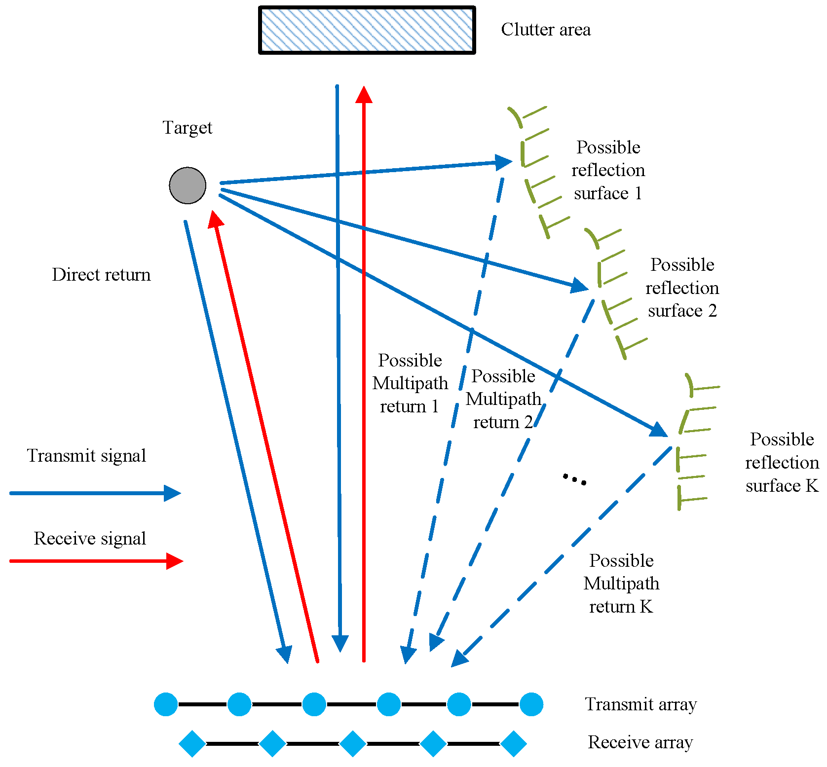
In our previous work [27], an MIMO jointly transmitted waveform and receiving filter design for multipath exploitation was investigated. Therein, the propagation path of the multipath return that was treated was known in advance, and the transmitted waveform and receiving filter could be optimized by leveraging the semi-definite relaxation, followed by a randomization procedure. Nevertheless, it is worth pointing out that the algorithm proposed in [27] is relatively limited in terms of its capability in more practical cases when the knowledge of the environment is incomplete or imprecise, i.e., the exact a priori knowledge on the multipath configuration (reflective coefficient of the surface, arrival direction, fast time delay) is unavailable. In this sense, signal model mismatches may happen, and the performance of the waveform designed in [27] is not guaranteed. Therefore, the design of a waveform that works against potential model mismatches to ensure robust performance is of great significance, and this remains an open issue.

Aiming at filling this gap, in this paper, we consider a robust MIMO waveform design to account for a more practical situation in which the prior knowledge about the multipath return is imperfect. Specifically, we assume that there are several possible expressions for the multipath return, depending on the position and reflective coefficient of the reflective surface. In this context, we consider the worst-case SINR at the outputs of the filter banks, with each tuned to a specific multipath return case, as the figure of merit in order to guarantee a robust target detection ability regardless of the actual multipath return. It is shown that the resultant robust design is hard to solve, since it belongs to a class of non-convex max–min optimization problems. We reformulated the design into an equivalent form that is easier to tackle and showed that the worst-case SINR can, thereby, be sequentially optimized based on a cyclic optimization procedure. At each iteration, when the signal is fixed, each element of the filter bank can be globally optimized, and the closed-form solution can be given directly; for a given filter bank, the waveform can be optimized by resorting to the generalized Dinkelbach algorithm [28,29]. At the analysis stage, the effectiveness of the proposed algorithm and its superiority over the non-robust design are illustrated through a series of developed case studies.

The remaining content of this paper is organized as follows. In Section 2, the signal model for the robust MIMO waveform design under unknown multipath return is introduced. In Section 3, the non-convex max–min problem for the joint robust design of the MIMO waveform and receiving filter bank is formulated, and a sequential optimization-based algorithm is proposed to obtain the optimized waveform and filters. Section 4 provides several numerical experiments to demonstrate the effectiveness and superiority of the proposed algorithm. Finally, Section 5 draws the conclusions and outlines some possible future research tracks.

Notations: Throughout this paper, scalars are denoted by italic letters; vectors and matrices are denoted by bold italic lowercase and capital letters, respectively. The operator tr(·) obtains the trace of a square matrix, and the operator vec(·) performs the column-wise stacking of a matrix. ${\mathbb{C}}^N$ stands for the N-dimensional complex space. $\Re \left(x\right)$ and $arg\left(x\right)$ obtain the the real part and phase angle of the argument x, respectively. ⊗ denotes the Kronecker product, and E(·) represents the expectation operator. The superscripts ${\left(·\right)}^T$ and ${\left(·\right)}^H$ denote the transpose and conjugate transpose, respectively. For a matrix $\mathbf{A}$, $\mathbf{A}\succ 0$ means that $\mathbf{A}$ is positive definite and $\mathbf{A}⪰0$ means that $\mathbf{A}$ is semi-definite.

2. Signal Model

Consider a colocated MIMO radar array consisting of $N_T$ transmitters and $N_R$ receivers that is deployed in a scene to detect a target in direction ${\theta }_t$. We denote its signal-transmitting matrix by $\mathbf{S}={[{\mathbf{s}}_1,{\mathbf{s}}_2,\dots ,{\mathbf{s}}_{N_T}]}^T\in {\mathbb{C}}^{N_T\times L}$, where ${\mathbf{s}}_n\in {\mathbb{C}}^L$ is the waveform transmitted at the nth channel, with L being the number of samples in fast time domain. As depicted in Figure 1, suppose that there is a reflective surface causing multipath return in the scenario. As a consequence, when the radar system transmits signals to illuminate the target, the echoes received by the array include not only the direct return, but also the backscattered target signal reflected from the reflective surface, which is defined as multipath return. There are also undesired returns from a cluttered area and other signal-independent disturbances. The echoes received by the radar are down-converted to the baseband, which can be expressed as

$$\mathbf{Y}={\mathbf{Y}}_d+{\mathbf{Y}}_m+{\mathbf{Y}}_c+\mathbf{n}\in {\mathbb{C}}^{N_R\times 2L},$$

(1)

where ${\mathbf{Y}}_d$, ${\mathbf{Y}}_m$, ${\mathbf{Y}}_c$, and $\mathbf{n}$ represent the direct return, multipath return, clutter, and noise, respectively. It is worth stressing that we focus on the received data, which consist of 2L-length range cells based on the model derived in [27], since longer propagation distances of the multipath return will lead to a longer fast time delay compared with the direct return.

2.1. Direct Return Model

The direct return signal from the target can be expressed as

$${\mathbf{Y}}_d={\alpha }_0{\mathbf{a}}_r\left({\theta }_d\right){\mathbf{a}}_t^T\left({\theta }_d\right)\mathbf{S}{\mathbf{J}}_0\in {\mathbb{C}}^{N_R\times 2L},$$

(2)

where ${\alpha }_0$ is a complex parameter accounting for the two-way direct propagation and backscattering effects from the target, and ${\mathbf{a}}_t\left({\theta }_d\right)\in {\mathbb{C}}^{N_T}$ and ${\mathbf{a}}_r\left({\theta }_d\right)\in {\mathbb{C}}^{N_R}$ represent, respectively, the transmitting and receiving steering vector in the target direction ${\theta }_d$. ${\mathbf{J}}_l$ is the $L\times 2L$ shift matrix, with its $(m,n)$th element given as

$${\mathbf{J}}_l(m,n)=\left\{\begin{array}{c}1,\mathrm{if}m-n+l=0\hfill \\ 0,\mathrm{if}m-n+l\ne 0\hfill \end{array}\right..$$

(3)

It is worth pointing out that the notation ${\mathbf{J}}_l$ is applied as a shift matrix for the rest of this paper. By utilizing the vectorization operator, we can obtain a $2N_{R}L\times 1$-dimensional direct return target vector that can be expressed as

$$\begin{array}{cc}\hfill & {\mathbf{y}}_d=\mathrm{vec}\left({\mathbf{Y}}_d\right)={\alpha }_0\underset{{\mathbf{H}}_d}{\underbrace{\left({\mathbf{J}}_0^T\otimes \left({\mathbf{a}}_r\left({\theta }_d\right){\mathbf{a}}_t^T\left({\theta }_d\right)\right)\right)}}\mathbf{s}\in {\mathbb{C}}^{2N_{R}L\times 1}\hfill \\ \hfill & ={\alpha }_0{\mathbf{H}}_d\mathbf{s},\hfill \end{array}$$

(4)

where $\mathbf{s}=\mathrm{vec}\left(\mathbf{S}\right)\in {\mathbb{C}}^{N_{T}L\times 1}$.

2.2. Multipath Return Model

In practice, accurate knowledge about a reflective surface (including its position and reflective coefficient) is not reasonable, and accordingly, it is more rational to assume that the actual multipath return has many possible expressions. To be specific, we assume that we know that the physical set of the reflective surface belongs to an uncertain set consisting of K possible cases, as shown in Figure 1. Accordingly, there are K possible formulations for the multipath return from the target in the direction ${\theta }_d$. Based on above analysis, we can get the baseband signal of the kth possible target multipath target return expression through slight modification of (2), which is expressed as

$${\mathbf{Y}}_{m,k}={\rho }_k{\alpha }_0{\mathbf{a}}_r\left({\theta }_{m,k}\right){\mathbf{a}}_t^T\left({\theta }_d\right)\mathbf{S}{\mathbf{J}}_{r_{m,k}}\in {\mathbb{C}}^{N_R\times 2L},$$

(5)

where ${\rho }_k$ and ${\theta }_{m,k}$ are, respectively, the corresponding reflective coefficient of the surface and the arrival direction of the multipath return. $r_{m,k}$ is the relative fast time delay of the kth possible path compared with the direct return.

Similarly to the derivation in (4), we can rewrite ${\mathbf{Y}}_{m,k}$ as a $2N_{R}L\times 1$ vector by resorting to the vectorization operator:

$$\begin{array}{cc}\hfill & {\mathbf{y}}_{m,k}=\mathrm{vec}\left({\mathbf{Y}}_{m,k}\right)={\rho }_k{\alpha }_0\underset{{\mathbf{H}}_{m,k}}{\underbrace{\left({\mathbf{J}}_{r_{m,k}}^T\otimes {\mathbf{a}}_r\left({\theta }_{m,k}\right){\mathbf{a}}_t^T\left({\theta }_d\right)\right)}}\mathbf{s}\in {\mathbb{C}}^{2N_{R}L\times 1}\hfill \\ \hfill & ={\rho }_k{\alpha }_0{\mathbf{H}}_{m,k}\mathbf{s}.\hfill \end{array}$$

(6)

2.3. Disturbance Model

In a radar operation, there are inevitable undesired reflections from other objects in the scene, e.g., the ground, water, and trees, which will have an obvious impact on the received echo. Herein, aside from the clutter within the same range cell as the target signal, we also take into consideration the impact of the clutter from the neighboring range cells. Therefore, the signal-dependent clutter is modeled as the superposition of signals from different directions and range cells. Suppose that there are P scatters in the scene interfering with the received echoes; then, based on the previous analysis, the clutter caused by the pth considered scatter can be expressed as

$${\mathbf{Y}}_{c,p}={\beta }_p{\mathbf{a}}_r\left({\theta }_p\right){\mathbf{a}}_t^T\left({\theta }_p\right)\mathbf{S}{\mathbf{J}}_{l_{c,p}}\in {\mathbb{C}}^{N_R\times 2L},$$

(7)

where ${\beta }_p$ represents the complex backscattering coefficient of the pth interfering object, ${\theta }_p$ is its relative direction with respect to (w.r.t) the radar, and $l_{c,p}$ is the relative fast time delay compared with the direct return. It should be pointed out that, here, we assume that no multipath return is involved in the clutter item. Hence, the total clutter item can be expressed as

$${\mathbf{Y}}_c=\sum _{p=1}^P{\beta }_p{\mathbf{a}}_r\left({\theta }_p\right){\mathbf{a}}_t^T\left({\theta }_p\right){\mathbf{SJ}}_{l_{c,p}}\in {\mathbb{C}}^{N_R\times 2L}.$$

(8)

Similarly to the derivations in the previous subsections, we write ${\mathbf{Y}}_c$ in vector form through column-wise stacking as follows:

$$\begin{array}{cc}\hfill {\mathbf{y}}_c=\mathrm{vec}\left({\mathbf{Y}}_c\right)& =\sum _{p=1}^P{\beta }_p\underset{{\mathbf{H}}_{c,p}}{\underbrace{\left({\mathbf{J}}_{l_{c,p}}^T\otimes \left({\mathbf{a}}_r\left({\theta }_p\right){\mathbf{a}}_t^T\left({\theta }_p\right)\right)\right)}}\mathbf{s}\hfill \\ & =\sum _{p=1}^P{\beta }_p{\mathbf{H}}_{c,p}\mathbf{s}\in {\mathbb{C}}^{2N_{R}L\times 1}.\hfill \end{array}$$

(9)

On the other hand, there are also signal-independent disturbances in the received data, which result from the system noise. Without loss of generality, we consider the signal-independent noise to be Gaussian, with its covariance matrix given as ${\mathbf{R}}_n$.

3. Problem Formulation and Proposed Algorithm

In addition to the various waveform design criteria, which include mutual information (MI) maximization [18,30,31], ambiguity function shaping [32,33,34,35], and Cramer–Rao-bound (CRB) minimization  [36,37], the SINR is widely utilized as the optimization criterion due to its close relationship with the target detection and parameter estimation performance [38,39,40]. In this context, we deal with the joint design of the transmitted waveform and the corresponding receiving filter bank by optimizing the worst-case SINR over the unknown multipath return for enhanced target detection performance. Unlike in the single-filter case, herein, our goal is to enhance the worst-case SINR, namely, the minimum SINR among the available branches, at the output of the filter bank. By doing this, we are able to improve the output SINR performance of the radar system in comparison with that of the conventional design regardless of the actual multipath return expression. Specifically, we propose the processing of the received data through a filter array consisting of K filters, with each filter being tuned to a specific multipath return case. As for the constraint imposed on the transmitted waveform, we restrict the waveform to have finite energy, i.e., ${\parallel \mathbf{s}\parallel }_2^2=1$. We denote by ${\mathbf{w}}_k$ the kth filter; its output SINR under the kth multipath return case can be calculated with

$$\begin{array}{cc}\hfill & {\mathrm{SINR}}_k=\frac{{\left|{\alpha }_0\right|}^2{\left|{\mathbf{w}}_k\left({\mathbf{H}}_d+{\rho }_k{\mathbf{H}}_{m,k}\right)\mathbf{s}\right|}^2}{{\mathbf{w}}_k^H\left({\displaystyle \sum _{p=1}^P}{\sigma }_{c,p}^2{\mathbf{H}}_{c,p}\mathbf{s}{\mathbf{s}}^H{\mathbf{H}}_{c,p}^H+{\mathbf{R}}_n\right){\mathbf{w}}_k}\hfill \end{array}.$$

(10)

where ${\sigma }_{c,p}^2=\mathrm{E}\left[|{\beta }_p{|}^2\right]$ is the interfering power of the pth scatter. Herein, the numerator of ${\mathrm{SINR}}_k$ denotes the useful energy at the output of the filter, and the denominator of ${\mathrm{SINR}}_k$ represents the remaining energy of the clutter and signal-independent noise. The worst-case SINR at the output of the filter bank is defined as

$$\begin{array}{cc}\hfill & \widetilde{\mathrm{SINR}}=\underset{k=1,\dots ,K}{min}{\mathrm{SINR}}_k\hfill \end{array}.$$

(11)

Based on the above analysis, the robust joint transmitted waveform and receiving filter bank design problem can be cast as

$$\mathcal{P}\left\{\begin{array}{c}\underset{\mathbf{s},{\left\{{\mathbf{w}}_k\right\}}_{k=1}^K}{max}\underset{k=1,\dots ,K}{min}\frac{{\left|{\alpha }_0\right|}^2{\left|{\mathbf{w}}_k^H\left({\mathbf{H}}_d+{\rho }_k{\mathbf{H}}_{m,k}\right)\mathbf{s}\right|}^2}{{\mathbf{w}}_k^H\left({\displaystyle \sum _{p=1}^P}{\sigma }_{c,p}^2{\mathbf{H}}_{c,p}\mathbf{s}{\mathbf{s}}^H{\mathbf{H}}_{c,p}^H+{\mathbf{R}}_n\right){\mathbf{w}}_k}\hfill \\ s.t.{∥\mathbf{s}∥}_2^2=1\hfill \end{array}\right..$$

(12)

It is seen that $\mathcal{P}$ is a non-convex problem (max–min objective and the energy constraint) and it NP-hard, which is difficult to solve. Nevertheless, as will be shown in the remainder of this part, a novel algorithm can be devised in order to effectively obtain a sub-optimal solution to $\mathcal{P}$. To begin with, the following proposition provides an equivalent formulation of $\mathcal{P}$, which lays the foundation for the subsequent derivations.

Proposition 1.

In terms of the optimal solution, Problem $\mathcal{P}$ is equal to the following problem:

$$\tilde{\mathcal{P}}\left\{\begin{array}{cc}\underset{\mathbf{s},{\left\{{\mathbf{w}}_k\right\}}_{k=1}^K}{max}\hfill & \underset{k=1,\dots ,K}{min}\frac{\left|{\alpha }_0\right|\Re \left({\mathbf{w}}_k^H\left({\mathbf{H}}_d+{\rho }_k{\mathbf{H}}_{m,k}\right)\mathbf{s}\right)}{\sqrt{{\mathbf{w}}_k^H\left({\displaystyle \sum _{p=1}^P}{\sigma }_{c,p}^2{\mathbf{H}}_{c,p}\mathbf{s}{\mathbf{s}}^H{\mathbf{H}}_{c,p}^H+{\mathbf{R}}_n{\parallel \mathbf{s}\parallel }_2^2\right){\mathbf{w}}_k}}\hfill \\ \hfill \hspace{1em}s.t.& \Re \left({\mathbf{w}}_k^H\left({\mathbf{H}}_d+{\rho }_k{\mathbf{H}}_{m,k}\right)\mathbf{s}\right)\ge 0,k=1,2,\dots ,K\hfill \end{array}\right..$$

(13)

This means that, once an optimal solution to $\tilde{\mathcal{P}}$ is obtained, it is possible to build an optimal solution to $\mathcal{P}$, and vice versa.

Proof. 

To begin with, it is obvious that the problem $\mathcal{P}$ shares the same optimal objective value with the following unconstrained max–min problem:

$$\begin{array}{cc}\hfill \underset{\mathbf{s},{\left\{{\mathbf{w}}_k\right\}}_{k=1}^K}{max}& \underset{k=1,\dots ,K}{min}\frac{{\left|{\alpha }_0\right|}^2{\left|{\mathbf{w}}_k^H\left({\mathbf{H}}_d+{\rho }_k{\mathbf{H}}_{m,k}\right)\frac{\mathbf{s}}{{\parallel \mathbf{s}\parallel }_2}\right|}^2}{{\mathbf{w}}_k^H\left({\displaystyle \sum _{p=1}^P}{\sigma }_{c,p}^2{\mathbf{H}}_{c,p}\frac{\mathbf{s}{\mathbf{s}}^H}{{\parallel \mathbf{s}\parallel }_2^2}{\mathbf{H}}_{c,p}^H+{\mathbf{R}}_n\right){\mathbf{w}}_k}\hfill \end{array}.$$

(14)

Moreover, since the value of the objective function in (14) is invariant by multiplying a scalar for the numerator and denominator at the same time, we can further recast (14) as

$$\begin{array}{cc}\hfill \underset{\mathbf{s},{\left\{{\mathbf{w}}_k\right\}}_{k=1}^K}{max}& \underset{k=1,\dots ,K}{min}\frac{{\left|{\alpha }_0\right|}^2{\left|{\mathbf{w}}_k^H\left({\mathbf{H}}_d+{\rho }_k{\mathbf{H}}_{m,k}\right)\mathbf{s}\right|}^2}{{\mathbf{w}}_k^H\left({\displaystyle \sum _{p=1}^P}{\sigma }_{c,p}^2{\mathbf{H}}_{c,p}\mathbf{s}{\mathbf{s}}^H{\mathbf{H}}_{c,p}^H+{\mathbf{R}}_n{\parallel \mathbf{s}\parallel }_2^2\right){\mathbf{w}}_k}\hfill \end{array}.$$

(15)

It is immediately ascertainable that (15) is equivalent to the following problem in the sense of optimal solutions:

$$\begin{array}{cc}\hfill & \underset{\mathbf{s},{\left\{{\mathbf{w}}_k\right\}}_{k=1}^K}{max}\underset{k=1,\dots ,K}{min}\frac{\left|{\alpha }_0\right|\left|{\mathbf{w}}_k^H\left({\mathbf{H}}_d+{\rho }_k{\mathbf{H}}_{m,k}\right)\mathbf{s}\right|}{\sqrt{{\mathbf{w}}_k^H\left({\displaystyle \sum _{p=1}^P}{\sigma }_{c,p}^2{\mathbf{H}}_{c,p}\mathbf{s}{\mathbf{s}}^H{\mathbf{H}}_{c,p}^H+{\mathbf{R}}_n{\parallel \mathbf{s}\parallel }_2^2\right){\mathbf{w}}_k}}\hfill \end{array}.$$

(16)

We denote the feasible points of (13) and (16) by ${\Omega }_1$ and ${\Omega }_2$, respectively. Then, it is obvious that ${\Omega }_1\subseteq {\Omega }_2$. Moreover, we note that, for any given point in ${\Omega }_1$, the objective value of (16) is larger than that of (13), which leads to the result that the optimal value of (16) is higher than that of (13). On the other hand, $\forall \overline{\mathbf{x}}=(\overline{\mathbf{s}},{\left\{{\overline{\mathbf{w}}}_k\right\}}_{k=1}^K)\in {\Omega }_2$, so one can verify that $\widehat{\overline{\mathbf{x}}}=(\overline{\mathbf{s}},{\left\{{\overline{\mathbf{w}}}_k·e^{jarg\left\{{\overline{\mathbf{w}}}_k^H\left({\mathbf{H}}_d+{\rho }_k{\mathbf{H}}_{m,k}\right)\overline{\mathbf{s}}\right\}}\right\}}_{k=1}^K)$ is in ${\Omega }_1$, and the objective in (13) achieves the same value at $\widehat{\overline{\mathbf{x}}}$ as the objective in (16) attains at $\overline{\mathbf{x}}$. That is to say, the optimal value of (13) is not lower than that of (16). In conclusion, (13) and (16) share the same optimal value, and any optimal solution for (13) is also optimal for (16). It is sufficient for us to deal with (13). Therefore, the proof is completed.    □

Based on Proposition 1, we can focus on dealing with $\tilde{\mathcal{P}}$ in the following content. Though the reformulated form $\tilde{\mathcal{P}}$ is still non-convex and NP-hard due to the max–min fractional objective function, in what follows, we develop an effective algorithm based on alternative optimization to obtain a sub-optimal solution to $\tilde{\mathcal{P}}$. In particular, at the nth iteration, we focus on tackling the problems of ${\tilde{\mathcal{P}}}_1^{\left(n\right)}$ and ${\tilde{\mathcal{P}}}_2^{\left(n\right)}$ w.r.t. the waveform and filters, respectively:

$${\tilde{\mathcal{P}}}_1^{\left(n\right)}\left\{\begin{array}{cc}\hfill \underset{{\left\{{\mathbf{w}}_k\right\}}_{k=1}^K}{max}& \underset{k=1,\dots ,K}{min}\frac{\left|{\alpha }_0\right|\Re \left({\mathbf{w}}_k^H\left({\mathbf{H}}_d+{\rho }_k{\mathbf{H}}_{m,k}\right){\mathbf{s}}^{(n-1)}\right)}{\sqrt{{\mathbf{w}}_k^H\left({\displaystyle \sum _{p=1}^P}{\sigma }_{c,p}^2{\mathbf{H}}_{c,p}{\mathbf{s}}^{(n-1)}{\mathbf{s}}^{(n-1)H}{\mathbf{H}}_{c,p}^H+{\mathbf{R}}_n{\parallel \mathbf{s}\parallel }_2^2\right){\mathbf{w}}_k}}\hfill \\ \hfill s.t.& \Re \left({\mathbf{w}}_k^H\left({\mathbf{H}}_d+{\rho }_k{\mathbf{H}}_{m,k}\right){\mathbf{s}}^{(n-1)}\right)\ge 0,k=1,2,\dots ,K\hfill \end{array}\right.$$

(17)

and

$${\tilde{\mathcal{P}}}_2^{\left(n\right)}\left\{\begin{array}{cc}\hfill \underset{\mathbf{s}}{max}& \underset{k=1,\dots ,K}{min}\frac{\left|{\alpha }_0\right|\Re \left({\mathbf{w}}_k^{\left(n\right)H}\left({\mathbf{H}}_d+{\rho }_k{\mathbf{H}}_{m,k}\right)\mathbf{s}\right)}{\sqrt{{\mathbf{w}}_k^{\left(n\right)H}\left({\displaystyle \sum _{p=1}^P}{\sigma }_{c,p}^2{\mathbf{H}}_{c,p}\mathbf{s}{\mathbf{s}}^H{\mathbf{H}}_{c,p}^H+{\mathbf{R}}_n{\parallel \mathbf{s}\parallel }_2^2\right){\mathbf{w}}_k^{\left(n\right)}}}\hfill \\ \hfill s.t.& \Re \left({\mathbf{w}}_k^{\left(n\right)H}\left({\mathbf{H}}_d+{\rho }_k{\mathbf{H}}_{m,k}\right)\mathbf{s}\right)\ge 0,k=1,2,\dots ,K\hfill \end{array}\right.,$$

(18)

where ${\mathbf{s}}^{\left(n\right)}$ and ${\left\{{\mathbf{w}}_k^{\left(n\right)}\right\}}_{k=1}^K$ denote the optimized waveform and filters at the nth iteration, respectively.

3.1. Optimizing Filters with a Fixed Waveform

Since ${\tilde{\mathcal{P}}}_1^{\left(n\right)}$ consists of K objective functions that are separable, we can proceed to dealing with the problem w.r.t. ${\mathbf{w}}_k$, which is formulated as

$${\tilde{\mathcal{P}}}_{1,k}^{\left(n\right)}\left\{\begin{array}{c}\underset{{\mathbf{w}}_k}{max}\frac{\left|{\alpha }_0\right|\Re \left({\mathbf{w}}_k^H\left({\mathbf{H}}_d+{\rho }_k{\mathbf{H}}_{m,k}\right){\mathbf{s}}^{(n-1)}\right)}{\sqrt{{\mathbf{w}}_k^H\left({\displaystyle \sum _{p=1}^P}{\sigma }_{c,p}^2{\mathbf{H}}_{c,p}{\mathbf{s}}^{(n-1)}{\mathbf{s}}^{(n-1)H}{\mathbf{H}}_{c,p}^H+{\mathbf{R}}_n\parallel {\mathbf{s}}^{(n-1)}{\parallel }_2^2\right){\mathbf{w}}_k}}\hfill \\ s.t.\Re \left({\mathbf{w}}_k^H\left({\mathbf{H}}_d+{\rho }_k{\mathbf{H}}_{m,k}\right){\mathbf{s}}^{(n-1)}\right)\ge 0\hfill \end{array}\right..$$

(19)

We denote by

$$\left\{\begin{array}{c}{\mathbf{d}}_k\left({\mathbf{s}}^{(n-1)}\right)=\left|{\alpha }_0\right|\left({\mathbf{H}}_d+{\rho }_k{\mathbf{H}}_{m,k}\right){\mathbf{s}}^{(n-1)}\hfill \\ \mathbf{Q}\left({\mathbf{s}}^{(n-1)}\right)=\sum _{p=1}^P{\sigma }_{c,p}^2{\mathbf{H}}_{c,p}^H{\mathbf{s}}^{(n-1)}{\mathbf{s}}^{(n-1)H}{\mathbf{H}}_{c,p}+{\mathbf{R}}_n\parallel {\mathbf{s}}^{(n-1)}{\parallel }_2^2\hfill \end{array}\right.$$

(20)

and recast the filter design problem as

$${\tilde{\mathcal{P}}}_{1,k}^{\left(n\right)}\left\{\begin{array}{cc}\hfill \underset{{\mathbf{w}}_k}{max}& \frac{\Re \left({\mathbf{w}}_k^H{\mathbf{d}}_k\left({\mathbf{s}}^{(n-1)}\right)\right)}{{\mathbf{w}}_k^H\mathbf{Q}\left({\mathbf{s}}^{(n-1)}\right){\mathbf{w}}_k}\hfill \\ \hfill s.t.& \Re \left({\mathbf{w}}_k^H{\mathbf{d}}_k\left({\mathbf{s}}^{(n-1)}\right)\right)\ge 0\hfill \end{array}\right..$$

(21)

One can easily verify that ${\tilde{\mathcal{P}}}_{1,k}^{\left(n\right)}$ is equivalent to the following problem:

$${\tilde{\mathcal{P}}}_{1,k}^{{\left(n\right)}^{\prime }}\left\{\begin{array}{cc}\hfill \underset{{\mathbf{w}}_k}{max}& {\mathbf{w}}_k^H\mathbf{Q}\left({\mathbf{s}}^{(n-1)}\right){\mathbf{w}}_k\hfill \\ \hfill s.t.& \Re \left({\mathbf{w}}_k^H{\mathbf{d}}_k\left({\mathbf{s}}^{(n-1)}\right)\right)=1\hfill \end{array}\right..$$

(22)

The optimal solution of the kth filter at the nth iteration can be immediately obtained [41], and it is given as

$$\begin{array}{c}\hfill {\mathbf{w}}_k^{\left(n\right)}={\mathbf{Q}}^{-1}\left({\mathbf{s}}^{(n-1)}\right)·{\mathbf{d}}_k\left({\mathbf{s}}^{(n-1)}\right)\end{array}.$$

(23)

3.2. Optimizing the Waveform with Fixed Filters

For fixed filters ${\left\{{\mathbf{w}}_k^{\left(n\right)}\right\}}_{k=1}^K$, the optimization problem of ${\mathbf{s}}^{\left(n\right)}$ is cast as

$${\tilde{\mathcal{P}}}_2^{\left(n\right)}\left\{\begin{array}{cc}\hfill \underset{\mathbf{s}}{max}& \underset{k=1,\dots ,K}{min}\frac{\left|{\alpha }_0\right|\Re \left({\mathbf{w}}_k^{\left(n\right)H}\left({\mathbf{H}}_d+{\rho }_k{\mathbf{H}}_{m,k}\right)\mathbf{s}\right)}{\sqrt{{\mathbf{w}}_k^{\left(n\right)H}\left({\displaystyle \sum _{p=1}^P}{\sigma }_{c,p}^2{\mathbf{H}}_{c,p}\mathbf{s}{\mathbf{s}}^H{\mathbf{H}}_{c,p}^H+{\mathbf{R}}_n{\parallel \mathbf{s}\parallel }_2^2\right){\mathbf{w}}_k^{\left(n\right)}}}\hfill \\ \hfill s.t.& \Re \left({\mathbf{w}}_k^{\left(n\right)H}\left({\mathbf{H}}_d+{\rho }_k{\mathbf{H}}_{m,k}\right)\mathbf{s}\right)\ge 0,k=1,2,\dots ,K\hfill \end{array}\right..$$

(24)

Note that the denominator of the objective in ${\tilde{\mathcal{P}}}_2^{\left(n\right)}$ can be equivalently formulated as

$$\begin{array}{cc}\hfill \sqrt{{\mathbf{w}}_k^{\left(n\right)H}\left(\sum _{p=1}^P{\sigma }_{c,p}^2{\mathbf{H}}_{c,p}\mathbf{s}{\mathbf{s}}^H{\mathbf{H}}_{c,p}^H+{\mathbf{R}}_n{\parallel \mathbf{s}\parallel }_2^2\right){\mathbf{w}}_k^{\left(n\right)}}& =\sqrt{{\mathbf{s}}^H\left(\sum _{p=1}^P{\sigma }_{c,p}^2{\mathbf{H}}_{c,p}^H{\mathbf{w}}_k^{\left(n\right)}{\mathbf{w}}_k^{\left(n\right)H}{\mathbf{H}}_{c,p}+{\mathbf{w}}_k^{\left(n\right)H}{\mathbf{R}}_n{\mathbf{w}}_k^{\left(n\right)}\right)\mathbf{s}}\hfill \\ & =\parallel {\left(\sum _{p=1}^P{\sigma }_{c,p}^2{\mathbf{H}}_{c,p}^H{\mathbf{w}}_k^{\left(n\right)}{\mathbf{w}}_k^{\left(n\right)H}{\mathbf{H}}_{c,p}+{\mathbf{w}}_k^{\left(n\right)H}{\mathbf{R}}_n{\mathbf{w}}_k^{\left(n\right)}\right)}^{\frac{1}{2}}{\mathbf{s}\parallel }_2\hfill \end{array}.$$

(25)

Therefore, we can reformulate ${\tilde{\mathcal{P}}}_2^{\left(n\right)}$ as

$${\tilde{\mathcal{P}}}_2^{{\left(n\right)}^{\prime }}\left\{\begin{array}{cc}\hfill \underset{\mathbf{s}}{max}& \underset{k=1,\dots ,K}{min}\frac{\left|{\alpha }_0\right|\Re \left({\mathbf{w}}_k^{\left(n\right)H}\left({\mathbf{H}}_d+{\rho }_k{\mathbf{H}}_{m,k}\right)\mathbf{s}\right)}{\parallel {\left({\displaystyle \sum _{p=1}^P}{\sigma }_{c,p}^2{\mathbf{H}}_{c,p}^H{\mathbf{w}}_k^{\left(n\right)}{\mathbf{w}}_k^{\left(n\right)H}{\mathbf{H}}_{c,p}+{\mathbf{w}}_k^{\left(n\right)H}{\mathbf{R}}_n{\mathbf{w}}_k^{\left(n\right)}\right)}^{\frac{1}{2}}{\mathbf{s}\parallel }_2}\hfill \\ \hfill s.t.& \Re \left({\mathbf{w}}_k^{\left(n\right)H}\left({\mathbf{H}}_d+{\rho }_k{\mathbf{H}}_{m,k}\right)\mathbf{s}\right)\ge 0,k=1,2,\dots ,K\hfill \end{array}\right..$$

(26)

It is obvious that ${\tilde{\mathcal{P}}}_2^{{\left(n\right)}^{\prime }}$ is non-convex. By defining the functions

$$\left\{\begin{array}{c}{u}_k^{\left(n\right)}\left(\mathbf{s}\right)=\left|{\alpha }_0\right|\Re \left({\mathbf{w}}_k^{\left(n\right)H}\left({\mathbf{H}}_d+{\rho }_k{\mathbf{H}}_{m,k}\right)\mathbf{s}\right)\hfill \\ v_k^{\left(n\right)}\left(\mathbf{s}\right)=\parallel {\left(\sum _{p=1}^P{\sigma }_{c,p}^2{\mathbf{H}}_{c,p}^H{\mathbf{w}}_k^{\left(n\right)}{\mathbf{w}}_k^{\left(n\right)H}{\mathbf{H}}_{c,p}+{\mathbf{w}}_k^{\left(n\right)H}{\mathbf{R}}_n{\mathbf{w}}_k^{\left(n\right)}\right)}^{\frac{1}{2}}{\mathbf{s}\parallel }_2\hfill \end{array}\right.,k=1,2,\dots ,K,$$

(27)

we can re-express ${\tilde{\mathcal{P}}}_2^{{\left(n\right)}^{\prime }}$ as

$${\tilde{\mathcal{P}}}_2^{{\left(n\right)}^{\prime }}\left\{\begin{array}{cc}\hfill \underset{\mathbf{s}}{max}& \underset{k=1,\dots ,K}{min}\frac{u_k^{\left(n\right)}\left(\mathbf{s}\right)}{v_k^{\left(n\right)}\left(\mathbf{s}\right)}\hfill \\ \hfill s.t.& u_k^{\left(n\right)}\left(\mathbf{s}\right)\ge 0,k=1,2,\dots ,K\hfill \end{array}\right..$$

(28)

It is worth noting that ${\tilde{\mathcal{P}}}_2^{{\left(n\right)}^{\prime }}$ is a typical generalized fractional programming problem ${\left\{u_k^{\left(n\right)}\left(\mathbf{s}\right)\right\}}_{k=1}^K$—are all non-negative concave functions; ${\left\{v_k^{\left(n\right)}\left(\mathbf{s}\right)\right\}}_{k=1}^K$—are all positive convex). Therefore, we propose that we tackle ${\tilde{\mathcal{P}}}_2^{{\left(n\right)}^{\prime }}$ by exploiting the idea of generalized Dinkelbach fractional programming. In detail, the approach involves an iteration process. At the qth iteration, the following problem is considered:

$${\mathcal{P}}_2^{(n,q)}\left\{\begin{array}{cc}\hfill \underset{\mathbf{s}}{max}& \underset{k=1,\dots ,K}{min}{u}_k^{\left(n\right)}\left(\mathbf{s}\right)-{\epsilon }^{(n,q-1)}{v}_k^{\left(n\right)}\left(\mathbf{s}\right)\hfill \\ \hfill s.t.& u_k^{\left(n\right)}\left(\mathbf{s}\right)\ge 0,k=1,2,\dots ,K\hfill \end{array}\right..$$

(29)

where ${\epsilon }^{(n,q-1)}={\displaystyle \underset{1\le k\le K}{min}}\frac{u_k^{\left(n\right)}\left({\mathbf{s}}^{(n,q-1)}\right)}{v_k^{\left(n\right)}{\left(\mathbf{s}\right)}^{(n,q-1)}}$, with ${\mathbf{s}}^{(n,q-1)}$ being the optimized waveform at the $(q-1)$th iteration. Subsequently, we will show that, by resorting to the epigraph form, $P_2^{(n,q)}$ can be recast into a maximization as

$${\mathcal{P}}_2^{{(n,q)}^{\prime }}\left\{\begin{array}{cc}\hfill \underset{\mathbf{s},t}{max}& t\hfill \\ \hfill s.t.& u_k^{\left(n\right)}\left(\mathbf{s}\right)\ge 0,\hfill \\ \hfill & u_k^{\left(n\right)}\left(\mathbf{s}\right)-{\epsilon }^{(n,q-1)}{v}_k^{\left(n\right)}\left(\mathbf{s}\right)\ge t,\hfill \\ \hfill & k=1,2,\dots ,K\hfill \end{array}\right..$$

(30)

where t is an auxiliary variable. It is seen that ${\mathcal{P}}_2^{{(n,q)}^{\prime }}$ is actually a second-order cone programming (SOCP) problem that can be solved in polynomial time via the interior point method. Based on the generalized Dinkelbach fractional programming paradigm, we can obtain a global optimal solution to ${\tilde{\mathcal{P}}}_2^{\left(n\right)}$ by solving a series of problems ${\left\{{\mathcal{P}}_2^{{(n,q)}^{\prime }}\right\}}_{q=1}^{\infty }$. For clearer illustration, we summarize the developed approach in Algorithm 1. It is worth stressing that ${\mathbf{H}}_d$, ${\left\{{\mathbf{H}}_{m,k}\right\}}_{k=1}^K$, ${\left\{{\rho }_k\right\}}_{k=1}^K$, ${\left\{{\mathbf{H}}_{c,p}\right\}}_{p=1}^P$, ${\left\{{\sigma }_{c,p}^2\right\}}_{p=1}^P$, and ${\mathbf{R}}_n$ are assumed to be known in advance.

Algorithm 1 Developed approach.
Input: ${\mathbf{H}}_d$, ${\left\{{\mathbf{H}}_{m,k}\right\}}_{k=1}^K$, ${\left\{{\rho }_k\right\}}_{k=1}^K$, ${\left\{{\mathbf{H}}_{c,p}\right\}}_{p=1}^P$, ${\left\{{\sigma }_{c,p}^2\right\}}_{p=1}^P$, ${\mathbf{R}}_n$
	Step 1.$n=0$, initialize the waveform ${\mathbf{s}}^{\left(0\right)}$.
	Step 2.$n=n+1$. Compute $\mathbf{Q}\left({\mathbf{s}}^{(n-1)}\right)$ and get the optimized kth filter as ${\mathbf{w}}_k^{\left(n\right)}={\mathbf{Q}}^{-1}\left({\mathbf{s}}^{(n-1)}\right)·{\mathbf{d}}_k\left({\mathbf{s}}^{(n-1)}\right)$.
	Step 3. Obtain the optimized waveform ${\mathbf{s}}^{\left(n\right)}$ by solving a series of SOCP problems ${\left\{{\mathcal{P}}_2^{{(n,q)}^{\prime }}\right\}}_{q=1}^{\infty }$
	Step 4. Repeat steps 2 and 3 until convergence.
Output Optimized waveform ${\mathbf{s}}^{\star }={\mathbf{s}}^{\left(n\right)}$ and filters ${\left\{{\mathbf{w}}_k^{\star }\right\}}_{k=1}^K={\left\{{\mathbf{w}}_k^{\left(n\right)}\right\}}_{k=1}^K$.

3.3. Complexity Analysis

As to the computational complexity of the proposed algorithm, it is dependent on the number of iterations and the complexity in each inner iteration. In particular, the overall complexity is linear w.r.t. the number of iterations, and it includes the computation of the matrix inversion and the solution of a series of SOCP problems in each iteration. While the optimization of the filters involves $\mathcal{O}\left({\left(2N_{R}L\right)}^3\right)$ floating-point operations, the optimization of the waveform is related to the number of inner iterations, and $\mathcal{O}\left({\left(2N_{T}L\right)}^{3.5}\right)$ floating-point operations are required for solving the SOCP problem ${\mathcal{P}}_2^{{(n,q)}^{\prime }}$ in each inner iteration [42].

4. Simulation Results

In this section, a series of examples are given to demonstrate the effectiveness of the proposed design. Specifically, we consider an MIMO radar with an inter-element spacing of $2d$ for both the transmitting and receiving array, where d is a half-wavelength. Throughout this part, the considered elements for the MIMO radar are fixed at $N_R=4$. The carrier frequency of the probing signals is set to 1 GHz, and the length of the code to be designed in each channel is set to $L=20$. As for the target, it is placed in the direction ${\theta }_d=-{20}^{\circ }$. With reference to the two-way direct propagation and backscattering effects from the target, ${\alpha }_0=1$ is set. We assume that there are $K=20$ possible reflective surface configurations in the scenario, accordingly resulting in 20 possible multipath return parameter pairs. Specifically, for the kth multipath return, ${\theta }_{m,k}$, $|{\rho }_k|$, and $arg\left({\rho }_k\right)$ are randomly drawn from the sectors $[-{30}^{\circ },0^{\circ }]$, $[0.92,0.94]$, and $[-\frac{\pi }{4},-\frac{\pi }{12}]$, and $r_{m,k}$ is drawn as a random integer from the region $[L-5,L]$. We consider the signal-independent disturbance to be white Gaussian noise with a uniting power of ${\sigma }_n^2=1$. For the signal-dependent item, we assume that there are $P=30$ scatters in the clutter area with azimuth directions ${\left\{{\theta }_p\right\}}_{p=1}^{30}$ that are uniformly drawn from the region $[-{90}^{\circ },{90}^{\circ }]$. The relative delay ${\left\{l_{c,p}\right\}}_{p=1}^{30}$ is uniformly drawn from integers in the region $[0,2L]$. The scatters are set to have the same mean interfering power ${\sigma }_{c,p}^2={\sigma }^2$, which is defined by the interference-to-noise ratio (INR), which is calculated as $\mathrm{INR}=10log\frac{{\sigma }^2}{{\sigma }_n^2}$. Throughout this part, the INR is set to 20 dB.

4.1. Convergence and Computation Time Analysis

In this example, we check the effectiveness of the developed algorithm on the sequentially improvement of the output worst-case SINR, as well as its convergence and computation time. As depicted in Figure 2, the worst-case SINR curves are plotted against the number of iterations for different transmitting array sizes $N_T$. As expected, the developed algorithm monotonically enhances the worst-case SINR, which significantly improves the target detection ability w.r.t. unknown multipath return. Furthermore, it is observed that a higher transmitting array size leads to a higher worst-case SINR due to the higher number of degrees of freedom (DOFs) that it introduces. Finally, the results shed light on the effectiveness of the developed algorithm in ensuring an optimized worst-case (w.r.t. unknown multipath return) target detectability. Indeed, significant performance gains through iterations can be explicitly observed. The corresponding computation times are reported in

Table 1. Computational times of the proposed algorithm with different transmitting array sizes.

${\mathit{N}}_{\mathit{T}}$	4	6	8	10
Computational time/s	627.077466	770.360833	1007.908756	1303.744407

. One can clearly observe that, though higher worst-case SINR values can be achieved as the transmitting array size becomes larger, the computational burden accordingly becomes heavier, which coincides with the complexity analysis in Section 3.3. Moreover, to illustrate the effectiveness of the proposed algorithm in optimizing the transmitted waveform more directly, we draw the modulus and the phase of the optimized waveform with different transmitting array sizes. As depicted in Figure 3, the waveforms optimized under different $N_T$ values exhibit different behaviors in the fast time domain, but all are constrained by the energy constraint.

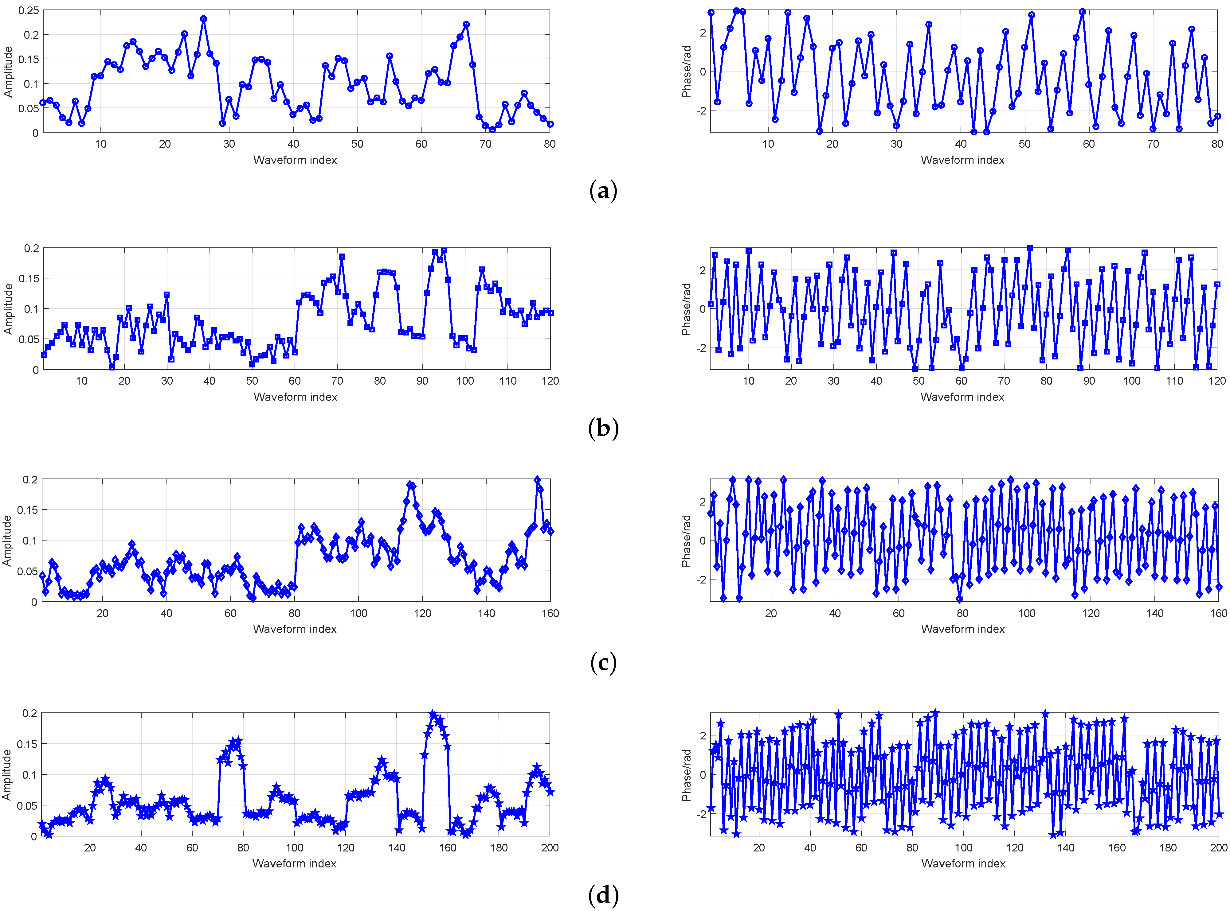
4.2. Robustness of the Developed Design against Different Multipath Returns

In this example, we further check the robustness of the waveforms and filters designed with the developed algorithm against the uncertainty of multipath return. In particular, we compute the actual achieved output SINR over various multipath returns with different transmitting array sizes. Moreover, for better illustration of the superiority of the proposed design, a non-robust design is added for comparison [27], which is defined as the solution to the following problem:

$$\left\{\begin{array}{c}\underset{\mathbf{s},\mathbf{w}}{max}\frac{{\left|{\alpha }_0\right|}^2{\left|\mathbf{w}\left({\mathbf{H}}_d+{\rho }_5{\mathbf{H}}_{m,5}\right)\mathbf{s}\right|}^2}{{\mathbf{w}}^H\left({\sum }_{p=1}^P{\sigma }_{c,p}^2{\mathbf{H}}_{c,p}\mathbf{s}{\mathbf{s}}^H{\mathbf{H}}_{c,p}^H+{\mathbf{R}}_n\right)\mathbf{w}}\hfill \\ s.t.{∥\mathbf{s}∥}_2^2=1\hfill \end{array}\right.$$

(31)

This means that we utilize the fifth multipath return case for the non-robust design. As shown in Figure 4, the worst-case output SINR provided by the proposed design significantly outperforms that of the non-robust design. Moreover, in these four situations, it can be observed that the proposed design provides a robust output SINR over various multipath propagation scenarios. The superiority of the proposed design is highlighted by observing that, in almost all multipath return cases, the SINR provided by the proposed design stayed around 3.5 dB higher than that of the non-robust design, except in the fifth multipath propagation case. This can be explained by the proposed design’s improvement of the worst-case SINR by averaging the performance over all possible cases, while the non-robust design was only effective in the fifth case. In practices, if there are mismatches between the models of the assumed and the actual scenarios, the performance of the non-robust design will be significantly degraded, but our design enjoys quite stable performance as the scenario changes. The results also show that a larger transmitting array size leads to a higher SINR value.

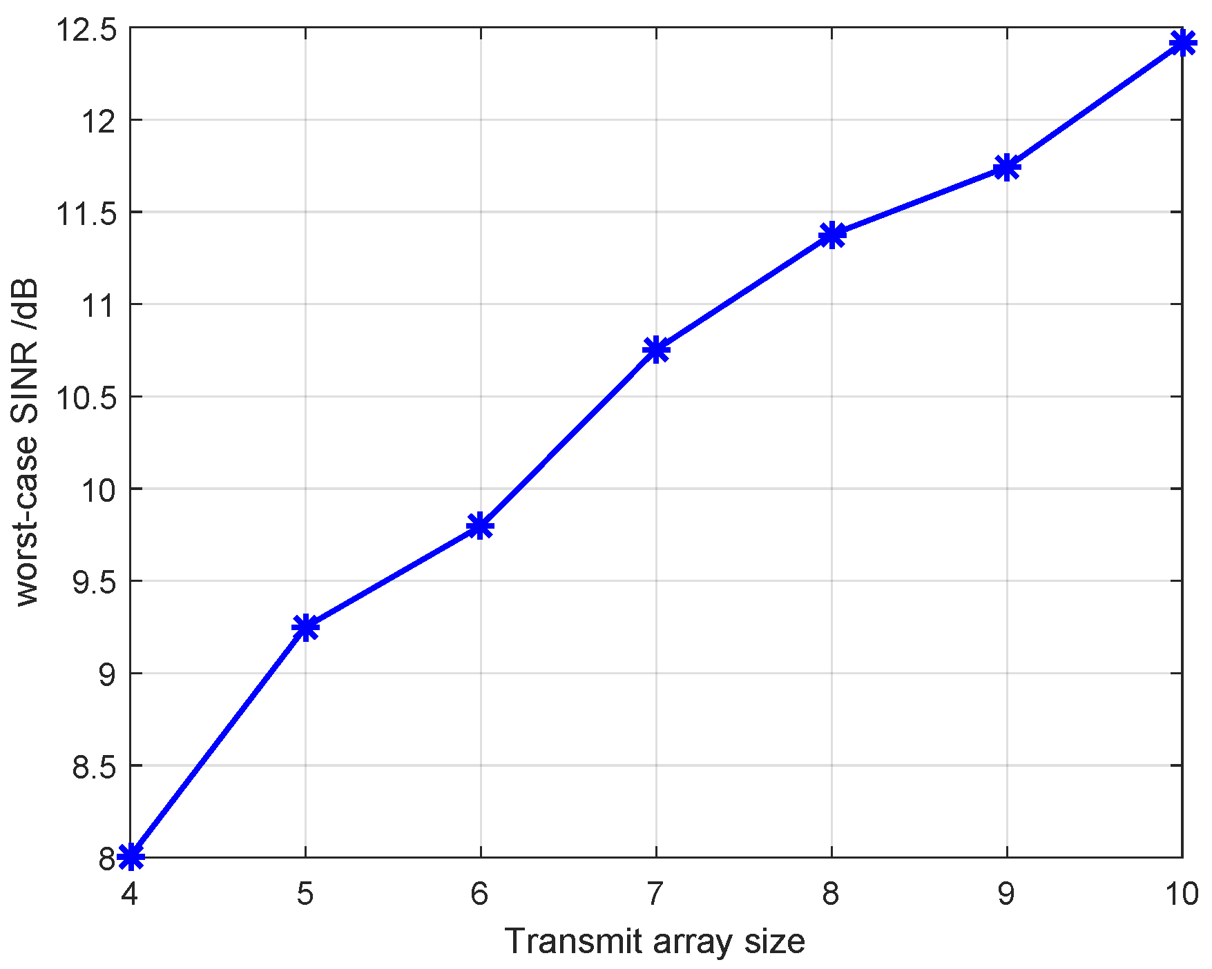
4.3. The Impact of the Transmitting Array Size on the Worst-Case SINR

In the final example, we check the impact of the transmitting array size $N_T$ on the worst-case SINR provided by the proposed algorithm. In particular, we plot the worst-case SINR curve with $N_T$ values varying from 4 to 10 in Figure 5, with the other parameters fixed. Unsurprisingly, the result clearly shows an increasing SINR trend w.r.t $N_T$, as a larger number of antennas can bring more DOFs in the waveform design process for disturbance suppression; consequently, higher worst-case SINR values can be obtained.

5. Conclusions

In this paper, a robust joint MIMO design for a transmitted waveform and receiving filter bank under uncertain multipath return was investigated. The goal of the robust design was to make the designed waveform and filters provide relatively stable output SINR values regardless of the actual multipath return expression, which was cast as a max–min problem and was hard to solve. A corresponding algorithm was developed based on a cyclic optimization paradigm. The simulation results show that the proposed design can achieve robustness against different multipath scenarios; this is of great significance in real applications, since actual information about an operating scene may be imprecise. Future research may include this robust design under more complex constraints on the transmitted waveform, such as spectral compatibility constraints.

References

1. Zhou, K.; Quan, S.; Li, D.; Liu, T.; He, F.; Su, Y. Waveform and filter joint design method for pulse compression sidelobe reduction. IEEE Trans. Geosci. Remote Sens. 2021, 60, 1–15. [Google Scholar] [CrossRef]
2. Yu, X.; Qiu, H.; Yang, J.; Wei, W.; Cui, G.; Kong, L. Multi-spectrally constrained MIMO radar beampattern design via sequential convex approximation. IEEE Trans. Aerosp. Electron. Syst. 2022, 58, 2935–2949. [Google Scholar] [CrossRef]
3. Argenti, F.; Facheris, L. Radar pulse compression methods based on nonlinear and quadratic optimization. IEEE Trans. Geosci. Remote Sens. 2020, 59, 3904–3916. [Google Scholar] [CrossRef]
4. Yang, J.; Aubry, A.; De Maio, A.; Yu, X.; Cui, G. Design of constant modulus discrete phase radar waveforms subject to multi-spectral constraints. IEEE Signal Process. Lett. 2020, 27, 875–879. [Google Scholar] [CrossRef]
5. Raei, E.; Alaee-Kerahroodi, M.; Shankar, M.B. Spatial-and range-ISLR trade-off in MIMO radar via waveform correlation optimization. IEEE Trans. Signal Process. 2021, 69, 3283–3298. [Google Scholar] [CrossRef]
6. Jiang, W.; Haimovich, A.M.; Simeone, O. Joint design of radar waveform and detector via end-to-end learning with waveform constraints. IEEE Trans. Aerosp. Electron. Syst. 2021, 58, 552–567. [Google Scholar] [CrossRef]
7. Liu, Q.; Ren, W.; Hou, K.; Long, T.; Fathy, A.E. Design of Polyphase Sequences with Low Integrated Sidelobe Level for Radars with Spectral Distortion via Majorization-Minimization Framework. IEEE Trans. Aerosp. Electron. Syst. 2021, 57, 4110–4126. [Google Scholar] [CrossRef]
8. Li, J.; Stoica, P. MIMO radar with colocated antennas. IEEE Signal Process. Mag. 2007, 24, 106–114. [Google Scholar] [CrossRef]
9. Li, J.; Stoica, P.; Xu, L.; Roberts, W. On parameter identifiability of MIMO radar. IEEE Signal Process. Lett. 2007, 14, 968–971. [Google Scholar]
10. Fishler, E.; Haimovich, A.; Blum, R.; Chizhik, D.; Cimini, L.; Valenzuela, R. MIMO radar: An idea whose time has come. In Proceedings of the 2004 IEEE Radar Conference (IEEE Cat. No. 04CH37509), Philadelphia, PA, USA, 29 April 2004; IEEE: Toulouse, France, 2004; pp. 71–78. [Google Scholar]
11. Yang, Y.; Blum, R.S. MIMO radar waveform design based on mutual information and minimum mean-square error estimation. IEEE Trans. Aerosp. Electron. Syst. 2007, 43, 330–343. [Google Scholar] [CrossRef]
12. He, H.; Stoica, P.; Li, J. Designing unimodular sequence sets with good correlations—Including an application to MIMO radar. IEEE Trans. Signal Process. 2009, 57, 4391–4405. [Google Scholar] [CrossRef]
13. Cheng, Z.; He, Z.; Zhang, S.; Li, J. Constant modulus waveform design for MIMO radar transmit beampattern. IEEE Trans. Signal Process. 2017, 65, 4912–4923. [Google Scholar] [CrossRef]
14. Cui, G.; Li, H.; Rangaswamy, M. MIMO radar waveform design with constant modulus and similarity constraints. IEEE Trans. Signal Process. 2013, 62, 343–353. [Google Scholar] [CrossRef]
15. Tang, B.; Tang, J. Joint design of transmit waveforms and receive filters for MIMO radar space-time adaptive processing. IEEE Trans. Signal Process. 2016, 64, 4707–4722. [Google Scholar] [CrossRef]
16. Aldayel, O.; Monga, V.; Rangaswamy, M. Successive QCQP refinement for MIMO radar waveform design under practical constraints. IEEE Trans. Signal Process. 2016, 64, 3760–3774. [Google Scholar] [CrossRef]
17. Cheng, Z.; He, Z.; Liao, B.; Fang, M. MIMO radar waveform design with PAPR and similarity constraints. IEEE Trans. Signal Process. 2017, 66, 968–981. [Google Scholar] [CrossRef]
18. Naghsh, M.M.; Modarres-Hashemi, M.; Kerahroodi, M.A.; Alian, E.H.M. An information theoretic approach to robust constrained code design for MIMO radars. IEEE Trans. Signal Process. 2017, 65, 3647–3661. [Google Scholar] [CrossRef]
19. Yu, X.; Cui, G.; Kong, L.; Li, J.; Gui, G. Constrained waveform design for colocated MIMO radar with uncertain steering matrices. IEEE Trans. Aerosp. Electron. Syst. 2018, 55, 356–370. [Google Scholar] [CrossRef]
20. Yu, X.; Alhujaili, K.; Cui, G.; Monga, V. MIMO radar waveform design in the presence of multiple targets and practical constraints. IEEE Trans. Signal Process. 2020, 68, 1974–1989. [Google Scholar] [CrossRef]
21. Aubry, A.; De Maio, A.; Foglia, G.; Orlando, D. Diffuse multipath exploitation for adaptive radar detection. IEEE Trans. Signal Process. 2015, 63, 1268–1281. [Google Scholar] [CrossRef]
22. Rong, Y.; Aubry, A.; De Maio, A.; Tang, M. Diffuse multipath exploitation for adaptive detection of range distributed targets. IEEE Trans. Signal Process. 2020, 68, 1197–1212. [Google Scholar] [CrossRef]
23. Richards, M.A. Principles of Modern Radar. Volume I, Basic Principles [Electronic Resource]; Richards, M.A., Scheer, J.A., Holm, W.A., Eds.; SciTech Pub.: Raleigh, NC, USA, 2010. [Google Scholar]
24. Fante, R.L.; Torres, J.A. Cancellation of diffuse jammer multipath by an airborne adaptive radar. IEEE Trans. Aerosp. Electron. Syst. 1995, 31, 805–820. [Google Scholar] [CrossRef]
25. Sen, S.; Nehorai, A. Adaptive OFDM radar for target detection in multipath scenarios. IEEE Trans. Signal Process. 2010, 59, 78–90. [Google Scholar] [CrossRef]
26. Sen, S.; Nehorai, A. OFDM MIMO radar with mutual-information waveform design for low-grazing angle tracking. IEEE Trans. Signal Process. 2010, 58, 3152–3162. [Google Scholar] [CrossRef]
27. Xu, Z.; Fan, C.; Huang, X. MIMO radar waveform design for multipath exploitation. IEEE Trans. Signal Process. 2021, 69, 5359–5371. [Google Scholar] [CrossRef]
28. Crouzeix, J.P.; Ferland, J.A. Algorithms for generalized fractional programming. Math. Program. 1991, 52, 191–207. [Google Scholar] [CrossRef]
29. Aubry, A.; De Maio, A.; Naghsh, M.M. Optimizing radar waveform and Doppler filter bank via generalized fractional programming. IEEE J. Sel. Top. Signal Process. 2015, 9, 1387–1399. [Google Scholar] [CrossRef]
30. Tang, B.; Liu, J.; Wang, H.; Hu, Y. Constrained radar waveform design for range profiling. IEEE Trans. Signal Process. 2021, 69, 1924–1937. [Google Scholar] [CrossRef]
31. Tang, B.; Li, J. Spectrally constrained MIMO radar waveform design based on mutual information. IEEE Trans. Signal Process. 2018, 67, 821–834. [Google Scholar] [CrossRef]
32. Cui, G.; Fu, Y.; Yu, X.; Li, J. Local ambiguity function shaping via unimodular sequence design. IEEE Signal Process. Lett. 2017, 24, 977–981. [Google Scholar] [CrossRef]
33. Li, Y.; Vorobyov, S.A.; Koivunen, V. Ambiguity function of the transmit beamspace-based MIMO radar. IEEE Trans. Signal Process. 2015, 63, 4445–4457. [Google Scholar] [CrossRef] [Green Version]
34. Arlery, F.; Kassab, R.; Tan, U.; Lehmann, F. Efficient gradient method for locally optimizing the periodic/aperiodic ambiguity function. In Proceedings of the 2016 IEEE Radar Conference (RadarConf), Philadelphia, PA, USA, 2–6 May 2016; IEEE: Toulouse, France, 2016; pp. 1–6. [Google Scholar]
35. Aubry, A.; De Maio, A.; Jiang, B.; Zhang, S. Ambiguity function shaping for cognitive radar via complex quartic optimization. IEEE Trans. Signal Process. 2013, 61, 5603–5619. [Google Scholar] [CrossRef]
36. Sen, S. PAPR-constrained pareto-optimal waveform design for OFDM-STAP radar. IEEE Trans. Geosci. Remote Sens. 2013, 52, 3658–3669. [Google Scholar] [CrossRef]
37. Li, J.; Xu, L.; Stoica, P.; Forsythe, K.W.; Bliss, D.W. Range compression and waveform optimization for MIMO radar: A Cramér–Rao bound based study. IEEE Trans. Signal Process. 2007, 56, 218–232. [Google Scholar]
38. Li, Z.; Shi, J.; Liu, W.; Pan, J.; Li, B. Robust joint design of transmit waveform and receive filter for MIMO-STAP radar under target and clutter uncertainties. IEEE Trans. Veh. Technol. 2021, 71, 1156–1171. [Google Scholar] [CrossRef]
39. Cui, G.; Fu, Y.; Yu, X.; Li, J.; Gui, G. Robust transmitter–receiver design for extended target in signal-dependent interference. Signal Process. 2018, 147, 60–67. [Google Scholar] [CrossRef]
40. Yang, J.; Aubry, A.; De Maio, A.; Yu, X.; Cui, G. Multi-spectrally constrained transceiver design against signal-dependent interference. IEEE Trans. Signal Process. 2022, 70, 1320–1332. [Google Scholar] [CrossRef]
41. Van Trees, H.L. Optimum Array Processing: Part IV of Detection, Estimation, and Modulation Theory; John Wiley & Sons: Hoboken, NJ, USA, 2004. [Google Scholar]
42. Ben-Tal, A.; Nemirovski, A. Lectures on Modern Monvex Mptimization (2012); SIAM: Philadelphia, PA, USA, 2011. [Google Scholar]
Figure 1. The considered scenario in the presence of multipath return.
Remotesensing 14 04356 g001
Figure 2. Worst-case SINR values of the waveform and filter with the proposed design versus the iteration number.
Remotesensing 14 04356 g002
Figure 3. Modulus and phase of the optimized waveform with different transmitting array sizes. (a) N T = 4 , (b) N T = 6 , (c) N T = 8 , and (d) N T = 10 .
Remotesensing 14 04356 g003
Figure 4. SINR values achieved with the proposed design and the non-robust design over different multipath propagation cases with various transmitting array sizes. (a) N T = 4 , (b) N T = 6 , (c) N T = 8 , and (d) N T = 10 .
Remotesensing 14 04356 g004
Figure 5. The worst-case output SINR provided by the proposed design versus the transmitting array size.
Remotesensing 14 04356 g005