Abstract
In modern electronic warfare, cognitive radar with knowledge-aided waveforms would show significant flexibility in anti-interference. In this paper, a novel method, named particle swarm-assisted projection optimization (PSAP), is introduced to design phase-coded waveforms with multi-level low range sidelobes, which mainly considers the stability for randomized initialization under the unimodular constraint. Firstly, the mathematical problem corresponding to avoid the range sidelobe masking from multiple non-cooperative targets or interference is formulated by giving different threat levels. Then, based on the alternating direction decomposition idea, the original problem is divided into triple-variable ones where these non-linear approximations can be solved via alternating projections along with FFT. Furthermore, the PSAP method with swarm intelligence, learning factor, and particle-assisted projection could ensure the optimization convergence in a parallel way, which could relax the non-convex constraint and enhance the global exploiting performance. Finally, simulations for several typical scenarios and numerical results are all provided to assess the waveforms generated by PSAP and other prevalent ones.
1. Introduction
Waveform diversity aided by high-performance radar hardware has received considerable attention and even made a great step forward to cognitive radar (CR) [1,2,3]. Most radars transmit a modulated waveform and then use some type of matched filter (MF) to enhance the signal-to-noise ratio (SNR) of the return echo. In mathematical sense, the MF output is usually the convolution between the received signal and the time-reversed replica of the transmitted signal, which is also regarded as the aperiodic auto-correlation [4,5,6]. Generally, to suppress range sidelobes which might obscure small targets of interest (especially, some dot targets or low RCS target) and further improve the anti-interference ability, the transmitting waveforms with desirable auto-correlation property are imperative by using some prior information [7,8,9,10]. Moreover, in engineering, the constant modulus (CM) of waveform (in most cases, i.e., unimodular property) could maximize the transmitter’s efficiency, but also makes the mathematical problem of generating waveform be more non-convex [11,12,13].
In the past 10 years, to achieve waveforms with ideal range sidelobes, minimizing integrated sidelobe level (ISL) and weighted integrated sidelobe level (WISL) have been developed as the classical metrics [14,15,16]. Therein, typical methods, such as cyclic algorithm new (CAN) [4], iterative spectral approximation algorithm (ISAA) [12], coordinate descent method (CD) [15], majorization minimization (MM) [16], weighted CAN (WeCAN) [17], alternating direction method of multipliers (ADMM) [18,19], etc., have also been presented and have received much attention. Note that, for mathematical problems under convex constraints, CANs could give some asymptotic convergence and make a big difference, while for the non-convex case CANs might stagnate into a suboptimum or local area [20,21]. Authors in [22] discussed the successive application of MM and phase gradient algorithm to synthesize the waveforms with low sidelobes. Additionally, authors adopted the limited memory Broyden–Fletcher–Goldfarb–Shanno algorithm (L-BFGS) to solve a fourth order polynomial formula and design unimodular sequences, but their ideas might incur invalidation for waveforms with large size [23]. Meanwhile, waveform optimization based on simulated annealing and stochastic neighborhood searching mechanism have also been presented, but these heuristic algorithms may be restricted to the modulus intricacy and large size of the waveforms [24,25].
Note that, when discussing the non-convex optimization with random initialization, these algorithms above would lead to a different terminus and only guarantee a local convergence [26]. Especially, to design the random phase-coded waveforms, how to tackle the random initialization for non-convex case has always been the key issue in engineering. Parallel optimization based on swarm intelligence maybe a good choice to improve the robustness. Unlike the optimization methods regarding each phase-coded unit, the waveform sample-based projection optimization using FFT will make a difference. In this paper, we use the idea of swarm particle intelligence [27,28,29] and combine alternating projection and particle swarm intelligence together to improve the global exploiting. To this end, our particle swarm-assisted projection optimization (PSAP) method is introduced to design the waveforms with desirable range sidelobes. Firstly, the mathematical problem is formulated to tackle the multiple non-cooperative targets or interference. Furthermore, using the alternating direction idea, the original problem is divided into some triple-variable ones considering different constraints. Then, the spectrum approximation in the sense of F-norm can be transformed into multi-variable alternating optimization cases. Finally, with the help of particle swarm intelligence, phase retrieval, learning factor and accelerated projections, PSAP method and its accelerated version have been formulated.
The remainder of paper is organized as follows. In Section 2, the system model is shown, and the formulated optimization problem for minimizing sidelobes is derived. In Section 3, PSAP as a novel alternative optimization mechanism based on swarm intelligence and FFT is presented. In Section 4, the performance of the proposed algorithms is evaluated and a series of numerical examples are also provided. Finally, in Section 5, the concluding remarks are provided.
2. The Signal Model and Problem Description
In this section, we discuss the range sidelobes masking effect from some strong RCS scatters which might obscure small targets of interest (such as dot target or low RCS target), and mainly focus on the waveform design for the static target detection in masking scenario and ignore the Doppler effect. For general description, the pre-modulated transmitting waveform in time domain has the discrete form of base band sequence with N code elements, i.e., . The received signal is down converted to base band and undergoes the MF at the receiver [30]. The vector format of autocorrelation function which can be regarded as the MF output at the zero Doppler shift, has been listed as follows
As shown in [12], suppose that a strong point scatterer (or the interference) with echo power exists in the q-th range cell, and a weak target of interest with echo power exists in the r-th range cell, the noise plus range sidelobe interference for the r-th range cell can be represented as
where , is the power of the thermal noise, and denotes the (q-r)-th lag of the aperiodic autocorrelation of (1). Then the target Signal power to Interference plus Noise Ratio (i.e., SINR) can be expressed as
here, of all the variables in (4), is the only one under the control of radar transmitter.
Despite the phase-coded waveform with arbitrary amplitude, the CM waveform could maximize the transmitter’s efficiency [13,16,31]. Let denote CM phase-coded one with discrete phase-coded units, i.e., where denotes the n-th phase-unit extracted from . , means the operation of transpose, complex conjugate, respectively. Similarly, we use to denote the range sidelobes of MF output in lieu of in (1) and (2). In modern electronic countermeasures scenarios, range sidelobes units occupied by some powerful interference or extended-scatters which mask the interesting target need to be suppressed [8,10,17]. Namely, local low range sidelobes is more convenient for weak targets detection and anti-masking effect as discussed in (3) and (4). Suppose that a powerful dot-scatter exists in the q-th range unit and inevitably impacts the target detection of the r-th one. With the help of some prior information , i.e., where denotes the area with a foreseeable target, we could further describe the range interval to be suppressed. We use an indicating vector 𝔃 to formulate the area-mapping of these pre-suppressed range sidelobes interval, i.e., when , and when . The classical weighted ISL given some prior information has been discussed in [4,7,17], i.e.,
Borrowed the idea of (5), we denote as the weight corresponding to each unit in 𝔃 , i.e., when , and when . We further define as the desirable waveform with ideal local low sidelobes, i.e., , denotes the Hadamard element-wise product. Let denote the approximation vector with . To design waveform with desirable property, namely, we should make and be more approximate. Here we use the norm-metric to denote the approximation level of them. Finally, the objective function can be formulated as
According to the “Parseval-type equality” in [17], i.e., , the objective function of (6) is equivalent to
where denotes the extend or cutoff matrix with , and refers to the frequency spectrum of and the designing one, respectively. The DFT matrix is constituted by unity exponential factor, i.e., with . Next, the optimization problem in (6) can be transformed into the spectrum approximation as following
Note that the problem of (9) is a quartic function of , using the auxiliary phase vector , (9) can be justified ‘almost equivalent’ to the following quadratic function of [17], i.e.,
and the ideal frequency spectrum vector can be further expressed as
As , (10) implies that once given , the ideal satisfies
namely, , so that will be constant once given x, then (10) in the vector format has
For brevity, defining a novel operator which rearranges the column vector to be a square diagonal matrix, i.e., , and the objective function (13) has
Similarly, given and , the quadratic optimization problem of (10) has
Let , then , (14) can be rewritten as
Meanwhile, is also an invertible matrix, the estimated in (16) could be given by
where represents the phase extractor from its vector argument, and denotes the imaginary component extraction operator. Similarly, recall “Parseval-type equality” again, the objective function in (15) could be expressed as:
On account of CM property, we only retain the phase section of the estimated of (18). Then the designed waveform by the phase-retrieval operation of [20] has
3. The Proposed Particles Swarm Assisted Projection Framework
In recent years, CAN [4], RISAAP [5], PONLP [12], CD [15], WeCAN [17], and ADMM [18] are all presented to deal with the Non-deterministic Polynomial-time hard (NP-hard) problem. They have the common trait, i.e., iterative optimization mechanism. Therein, each iteration of them requires to solve a non-convex problem under unimodular constraint, no matter by virtue of handling the bisection gradient optimization or FFT-based one. However, the initialized random phases where each phase unit is distributed in , would incur a different terminus when using different random initialization. Namely, each Monte-Carlo trial could obtain different solution and remain some local convergence. To tackle these, we borrow the idea of parallel optimization to combine the particles swarm intelligence and projection optimization together, where the novel particles projection mechanism will avoid the local area in the statistical sense. Next, we present the PSAP framework in lieu of the traditional evolution mechanism of PSO or DE [28,29], and thus could enhance the global exploiting for non-convex phase-coded problem. The detailed descriptions of PSAP have been listed as follows
Step 1. Formulate the waveform set rather than one single sequence, i.e., with . Note that each sequence has , where denotes the independent phase-coded variables extracted from . Additionally, the waveform set could also be initialized by Frank or Barker sequence.
Step 2. Define a novel metric to assess the sidelobe performance of waveform in the range interval as
where denotes the number of pre-suppressed sidelobes units.
Step 3. Using (20) as the fitness function to evaluate each waveform of set , and select the best fitness function and its corresponding waveform .
Step 4. For the t-th iteration, select waveforms from waveform set to formulate the novel subset. Here we should update the subset by some rules that if the best fitness function and its corresponding waveform have not been incorporated, then use it to replace the worst one in current subset.
Step 5. For each waveform at the t-th iteration, utilize the oversampling FFT to get , and then formulate the relaxing factor , relational factor , and also projection vector by using (22)~(24) respectively, as follows
where denotes the relational factor of the m-th waveform at the t-th iteration to the t + 1-th iteration, denotes one random value of [0, 1], represent the inertia factor, is the learning factor related to the best waveform which is selected from initial iteration to the current iteration . represents the learning factor related to the best waveform at the current t-th iteration.
Step 6. Use the multi-particles projection of (25)~(26) to achieve unimodular waveforms at the t + 1-th iteration, as follows
where with CM property has been obtained by the phase retrieval operation in (26).
Step 7. Consider the remaining subset, update them by
Step 8. Merge the subset and remaining part, use the following selection rules to get , i.e., when , or not , and select the best fitness function and its corresponding waveform .
Step 9. Repeat step 3~8 until or num > iter_num, then output . Otherwise, update t = t + 1 and continue iterating.
Furthermore, we could incorporate the gradient steepest idea into PSAP. The objective function of (15) can be expressed as:
Let , then the two-variable optimization problem has
Given the latest iterative , can be achieved by the follow gradient optimization, and its gradient matrix has
Let (32) equal to 0, then has:
where , as known, only if is the even value, the hessian matrix of (33) can be positive, and (30) will get the minimum. Moreover, given , the phase vector of has:
Finally, the detailed descriptions of particle swarm-assisted projection with optimizing mechanism (named as PSAPOM) have been listed as follow:
Step 1~Step 3 are similar to PSAP.
Step 4. Define , then calculate the gradient direction , then search the best length which satisfies
define , then
if or , output the initiation ;
Step 5. For the current iteration, select waveforms from set to formulate the novel subset. Here we should update the subset by some rules that if the best fitness function and its corresponding waveform have not been incorporated, then use it to replace the worst one in current subset.
Step 6. For each waveform of subset, utilize the oversampling FFT to get , and then formulate the relaxing factor , relational factor , and also projection vector by using (39)~(41) respectively, as follows
where denotes the relational factor of the m-th waveform at the t-th iteration to the t + 1-th iteration, denotes one random value in [0, 1], represent the inertia factor, is the learning factor related to the best waveform which is chosen from initial iteration to the current iteration . represents the learning factor related to the best waveform at the current t-th iteration.
Step 7. Use the multi-particles projection to achieve unimodular waveforms at t + 1-th iteration,
where with CM property has been obtained by the phase retrieval operation of (43).
Step 8. For the remaining subset, update them by
Step 9. Merge the subset and the remaining part, use the following rules to get , i.e.,
then select the best fitness function and its corresponding waveform .
Step 10. Repeat above-mentioned steps 5~9 until num > iter_num or , then output . Otherwise, update t = t + 1 and continue iterating.
4. Simulations and Performance Analysis
Note that the non-convex optimization problem under different initialization is usually providing a different terminus, and hard to obtain the global solution within polynomial time [5,11,26]. For the phase-coded CM waveform design, selecting an effective technique has always been the focus [12,13,14]. In this section, to further assess PSAP’s performance, we firstly assume code length of waveform , then the initialized waveform set has
where , . In addition, the inertia weight, individual learning factor as well as group learning factor are set as , , and , respectively. The iterations number iter_num is set as 2000, threshold value of is set as .
Next, we take the scenario of suppressing one single area for comparison, i.e., single interval . PSAP will be compared with WeCAN, ISAA, RISAAP, and PONLP, by 20 Monte Carlo (MC) trials. Here, we define the averaging autocorrelation sidelobe level (Aver-ACL) and local PSL (LPSL) in suppressed regions as the metric, as follows
for the sake of comparison, all methods or algorithms would be initialized by random phase-coded sequence. Performance comparisons have been shown in Table 1 and Figure 1. Simulations are performed on a PC with 3.40 GHz i7 CPU.

Table 1.
Performance comparison for suppressing single area sidelobes of different algorithms.
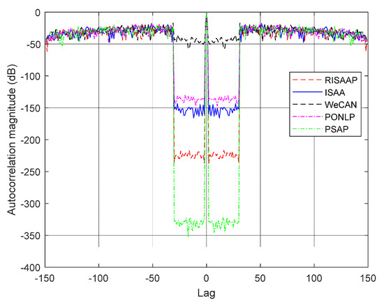
Figure 1.
ACL comparison for suppressing sidelobes in a single area.
In Table 1 and Figure 1, our proposed PSAP with parallel optimization mechanism has achieved the best performance, PONLP with stochastic gradient optimization has achieved only −139 dB of Aver-ACL and −130 dB of LPSL, while WeCAN achieves −48 dB of Aver-ACL and −35 dB of LPSL. Moreover, ISAA and RISAAP using the mechanism of alternating projection has obtained −228 dB and −158 dB of Aver-ACL, −216 dB and −144 dB of LPSL, respectively. We need to declare that, with as the mathematical metric referring to [4,5,12,17], these methods or algorithms conduct their iterating or optimizing with the same stop criteria/thresholds (iter_num is set as 2000, threshold value is set as ). Here, the phenomenon with –228 dB or −333 dB may be unnecessary to have so low sidelobe levels for practical engineering, but these low values in mathematical sense would demonstrate some quickly converging or optimizing level of our PSAP framework even for the future electronic countermeasure scenario.
To further discuss the computation complexity of them, here we mainly demonstrate the number of iterations in convergence graph (as shown in Figure 2), and the CPU time consumption in Table 1. In Figure 2, we use as the convergence metric of the y-coordinate. Figure 2 has shown obvious converging difference. PSAP uses the idea of particles swarm intelligence, i.e., M = 20, to establish thus cooperative optimization (in CPU model), also occupies much more time than RISAAP, ISAA and PONLP. WeCAN has consumed the longest time 5.11 s. By 20 MC trails, we can see that PSAP has achieved the best robustness performance, which is own to the parallel cooperative mechanism. In addition, these trails and simulations are all based on CPU; when given the GPU condition, PSAP will occupy much less time than others. As seen in Table 1 and Figure 2, WeCAN has slow convergence and PONLP with the steepest descent gradient might stagnate into the local area. ISAA and RISAAP have oscillations in Figure 2 which might attribute to the alternating projection between multi-local areas for the non-convex case.
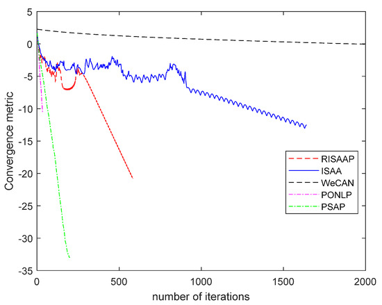
Figure 2.
Convergence comparison of different methods.
In addition, we also discuss the Aver-ACL and LPSL comparisons with different code lengths N (i.e., 150, 200, 250, 300) which are shown in Figure 3. No matter N = 150, 200, 250, and 300, our proposed PSAP could obtain the best Aver-ACL and LPSL in different code lengths. Meanwhile, the results of these methods in Figure 3 have shown some similarity that WeCAN might lose the performance for engineering application.
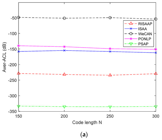
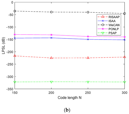
Figure 3.
Aver-ACL and LPSL comparison with different code lengths N. (a) Aver-ACL comparison of RISAAP, ISAA, WeCAN, PONLP, and PSAP. (b) LPSL comparison of RISAAP, ISAA, WeCAN, PONLP, and PSAP.
Meanwhile, we also consider the sidelobe suppression in multiple-area case, i.e., . Here, we assign different suppressing levels with where the former corresponds to the range sidelobe area next to the mainlobe, and the second refers to the farther one. Note that, the interferences near the mainlobe would also produce more effect than the farther one, and affect the detecting performance. Namely, we arrange two suppressing areas with different weights to demonstrate the suppressing levels for different non-cooperative targets. When discussing , the former with relative-low weights means more emphasis on the first area. In Table 2 and Figure 4, we could see that the first area has achieved more excellent performance than the second one, which is due to the weights of the different non-cooperative targets.
Table 2.
Performance comparison for suppressing multiple area sidelobes with different weights.
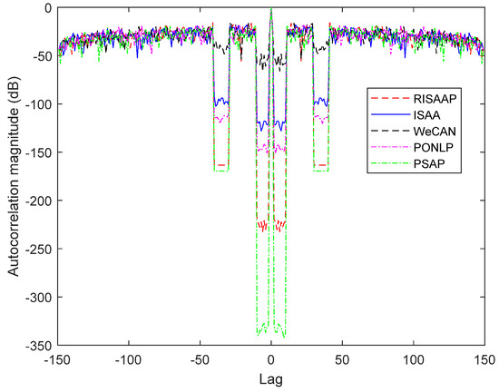
Figure 4.
ACL comparison for suppressing sidelobes for multiple areas.
In Table 2 with recorded time-consumption data, obviously, our proposed PSAP with 0.84 s has achieved the best Aver-ACL and LPSL using 20 MC trials, but with more time than RISAAP (with 0.16 s), ISAA (with 0.34 s) and PONLP (with 0.45 s). Moreover, WeCAN (with 5.94 s) has lost the performance and cost more time than others.
Moreover, we also consider the multiple-case, i.e., and arrange two suppressing areas with same weights . In Table 3 and Figure 5, we could see that these two areas have achieved same excellent performance. Table 3 has shown same characteristics as shown in Table 1 and Table 2. Our proposed PSAP has achieved the best result by 20 MC trials. WeCAN has lost its performance.
Table 3.
Performance comparison for suppressing multiple area sidelobes with same weights.
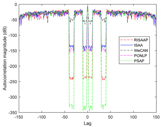
Figure 5.
ACL comparison of suppressing sidelobes for multiple areas.
Note that the initialization of algorithms is indeed significant no matter for cyclic algorithms or alternating projection. As the Gradient Descent (GD) mechanism could accelerate the exploiting for local optimization, and we combine the GD and PSAP together to formulate the PSAPOM and enhance the global robustness. To further assess the performance of PSAPOM and PSAP, despite the random phase-coded sequence, here we assume that these algorithms have been initialized by the Frank-coded or Barker-coded sequence, respectively. For the length (N = 196), the Frank sequence is given by:
we also assume another waveform sequence (N = 169) formulated by the 13 Barker sequence. As shown in Figure 6 and Table 4, for both the Frank sequence and Barker sequence, PSAPOM also achieved the same performance as PSAP, but its time consumption, 0.4210 s and 0.2502 s, was less than PSAP.
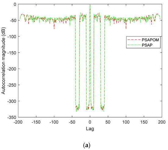
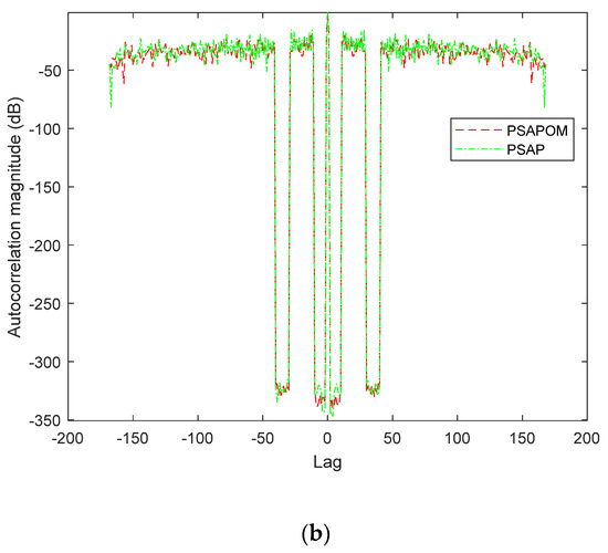
Figure 6.
ACL performance comparison for suppressing multiple sidelobe areas. (a) Description of PSAPOM and PSAP initialized by Frank-coded sequence; (b) Description of PSAPOM and PSAP initialized by the 13 Barker-coded sequence.
Table 4.
Algorithm (initialized by the Frank or Barker sequence) comparison for suppressing range sidelobes.
In these comparisons, we could draw a basic conclusion that our improved PSAP algorithms have a remarkable performance compared to WeCAN, PONLP, ISAA, and RISAAP, which will have a large influence on future practical applications. Moreover, given the sophisticated scenarios, i.e., the unimodular constraint and multiple suppressing areas, our PSAP and PSAPOM have shown a more powerful convergence than these methods. Meanwhile, our simulations have demonstrated that PSAP and PSAPOM have excellent robustness and stability. We may attribute these traits to FFT leverage and swarm particle intelligence due to alternating projection mechanisms.
5. Conclusions
In this paper, a PSAP framework (such as PSAP and PSAPOM) is introduced to design a unimodular CM phase-coded waveform with local low range sidelobes. Therein, PSAP with learning factor and particle-assisted projection could improve the convergence in the non-convex case. Numerical trails and simulations have also provided plenty of analysis to assess the waveforms generated by PSAP, WeCAN, ISAA, RISAAP, and PONLP. Regarding statistical performance, PSAP and PSAPOM via swarm intelligence and parallel optimization idea have achieved outstanding results. Additionally, in this paper, as we only discussed the masking scenarios of detecting static targets despite the Doppler effect of moving targets, in our further research, we will continue designing other phase-coded waveforms considering the non-zero Doppler effect. Moreover, we will also use GPU to accelerate the distributed parallel optimization.
Author Contributions
Conceptualization, X.F. and F.L.; Data curation, X.F.; Formal analysis, F.L., W.C. and Z.Z.; Funding acquisition, Z.Z.; Investigation, F.L. and Y.Z.; Methodology, X.F., F.L., W.C., Z.Z. and Y.Z.; Project administration, X.F. and Y.Z.; Resources, Z.Z.; Supervision, Z.Z.; Validation, F.L. and W.C.; Writing—original draft, X.F. and W.C.; Writing—review and editing, X.F. and Y.Z. All authors have read and agreed to the published version of the manuscript.
Funding
This research was funded by the National Natural Science Foundation of China, grant number 42127804.
Data Availability Statement
Not applicable.
Acknowledgments
We also appreciate the anonymous reviewers.
Conflicts of Interest
The authors declare no conflict of interest.
References
- Blunt, S.D.; Mokole, E.L. Overview of radar waveform diversity. IEEE Aerosp. Electron. Syst. Mag. 2016, 31, 2–42. [Google Scholar] [CrossRef]
- Guolong, C.; Xianxiang, Y.; Jing, Y.; Yue, F.; Lingjiang, K. An Overview of Waveform Optimization Methods for Cognitive Radar. J. Radars 2019, 8, 537–557. [Google Scholar]
- Li, Y.; Vorobyov, S.A. Fast algorithms for designing unimodular waveform(s) with good correlation properties. IEEE Trans. Signal Process. 2017, 66, 1197–1212. [Google Scholar] [CrossRef]
- Stoica, P.; He, H.; Li, J. New algorithms for designing unimodular sequences with good correlation properties. IEEE Trans. Signal Process. 2009, 57, 1415–1425. [Google Scholar] [CrossRef]
- Feng, X.; Zhao, Y.; Zhou, Z.; Zhao, Z.-F. Waveform design with low range sidelobe and high Doppler tolerance for cognitive radar. Signal Process. 2017, 139, 143–155. [Google Scholar] [CrossRef]
- Kajenski, P.J. Design of low-sidelobe phase-coded waveforms. IEEE Trans. Aerosp. Electron. Syst. 2019, 55, 2891–2898. [Google Scholar] [CrossRef]
- Bu, Y.; Yu, X.; Yang, J.; Fan, T.; Cui, G. A new approach for design of constant modulus discrete phase radar waveform with low WISL. Signal Process. 2021, 187, 108145. [Google Scholar] [CrossRef]
- Fan, W.; Liang, J.; Yu, G.; So, H.C.; Lu, G. Minimum local peak sidelobe level waveform design with correlation and/or spectral constraints. Signal Process. 2020, 171, 107450. [Google Scholar] [CrossRef]
- Bolhasani, M.; Mehrshahi, E.; Ghorashi, S.A.; Alijani, M.S. Constant envelope waveform design to increase range resolution and SINR in correlated MIMO radar. Signal Process. 2019, 163, 59–65. [Google Scholar] [CrossRef]
- Thakur, A.; Saini, D.S. MIMO radar sequence design with constant envelope and low correlation side-lobe levels. AEU-Int. J. Electron. Commun. 2021, 136, 153769. [Google Scholar] [CrossRef]
- Song, J.; Babu, P.; Palomar, D.P. Optimization methods for designing sequences with low autocorrelation sidelobes. IEEE Trans. Signal Process. 2015, 63, 3998–4009. [Google Scholar] [CrossRef] [Green Version]
- Li, F.; Zhao, Y.; Qiao, X. A waveform design method for suppressing range sidelobes in desired intervals. Signal Process. 2014, 96, 203–211. [Google Scholar] [CrossRef]
- Ge, P.; Cui, G.; Karbasi, S.M.; Kong, L.; Yang, J. A template fitting approach for cognitive unimodular sequence design. Signal Process. 2016, 128, 360–368. [Google Scholar] [CrossRef]
- Aubry, A.; De Maio, A.; Jiang, B.; Zhang, S. Ambiguity function shaping for cognitive radar via complex quartic optimization. IEEE Trans. Signal Process. 2013, 61, 5603–5619. [Google Scholar] [CrossRef]
- Kerahroodi, M.A.; Aubry, A.; De Maio, A.; Naghsh, M.M.; Modarres-Hashemi, M. A coordinate-descent framework to design low PSL/ISL sequences. IEEE Trans. Signal Process. 2017, 65, 5942–5956. [Google Scholar] [CrossRef]
- Esmaeili-Najafabadi, H.; Leung, H.; Moo, P.W. Unimodular waveform design with desired ambiguity function for cognitive radar. IEEE Trans. Aerosp. Electron. Syst. 2019, 56, 2489–2496. [Google Scholar] [CrossRef]
- He, H.; Li, J.; Stoica, P. Waveform Design for Active Sensing Systems: A Computational Approach; Cambridge University Press: Cambridge, UK, 2012. [Google Scholar]
- Cheng, Z.; Liao, B.; He, Z.; Li, J.; Han, C. A nonlinear-ADMM method for designing MIMO radar constant modulus waveform with low correlation sidelobes. Signal Process. 2019, 159, 93–103. [Google Scholar] [CrossRef]
- Liu, Y.; Jiu, B.; Liu, H. ADMM-based transmit beampattern synthesis for antenna arrays under a constant modulus constraint. Signal Process. 2020, 171, 107529. [Google Scholar] [CrossRef]
- Patton, L.K.; Rigling, B.D. Phase retrieval for radar waveform optimization. IEEE Trans. Aerosp. Electron. Syst. 2012, 48, 3287–3302. [Google Scholar] [CrossRef]
- Zhang, X.; Wang, X. Waveform design with controllable modulus dynamic range under spectral constraints. Signal Process. 2021, 189, 108285. [Google Scholar] [CrossRef]
- Wu, Z.J.; Zhou, Z.Q.; Wang, C.X.; Li, Y.-C.; Zhao, Z.-F. Doppler resilient complementary waveform design for active sensing. IEEE Sens. J. 2020, 20, 9963–9976. [Google Scholar] [CrossRef]
- Wang, Y.C.; Dong, L.; Xue, X.; Yi, K.-C. On the design of constant modulus sequences with low correlation sidelobes levels. IEEE Commun. Lett. 2012, 16, 462–465. [Google Scholar] [CrossRef]
- Xue-Bin, S.; Zhan-Min, L.; Cheng-Lin, Z.; Zheng, Z. Cognitive UWB Pulse Waveform Design Based on Particle Swarm Optimization. Adhoc Sens. Wirel. Netw. 2012, 16, 215–228. [Google Scholar]
- Wang, S. Efficient heuristic method of search for binary sequences with good aperiodic autocorrelations. Electron. Lett. 2008, 44, 731–732. [Google Scholar] [CrossRef]
- Zhao, D.; Wei, Y.; Liu, Y. Design of unimodular sequence train with low central and recurrent autocorrelations. IET Radar Sonar Navig. 2018, 13, 45–49. [Google Scholar] [CrossRef]
- Tanweer, M.R.; Suresh, S.; Sundararajan, N. Self regulating particle swarm optimization algorithm. Inf. Sci. 2015, 294, 182–202. [Google Scholar] [CrossRef]
- Zhang, H.; Xie, J.; Zong, B. Bi-objective particle swarm optimization algorithm for the search and track tasks in the distributed multiple-input and multiple-output radar. Appl. Soft Comput. 2021, 101, 107000. [Google Scholar] [CrossRef]
- Lin, R.; Soltanalian, M.; Tang, B.; Li, J. Efficient design of binary sequences with low autocorrelation sidelobes. IEEE Trans. Signal Process. 2019, 67, 6397–6410. [Google Scholar] [CrossRef]
- Levanon, N.; Mozeson, E. Radar Signals; John Wiley & Sons: Hoboken, NJ, USA, 2004. [Google Scholar]
- Klauder, J.R.; Price, A.C.; Darlington, S.; Albersheim, W.J. The theory and design of chirp radars. Bell Syst. Tech. J. 1960, 39, 745–808. [Google Scholar] [CrossRef]
Publisher’s Note: MDPI stays neutral with regard to jurisdictional claims in published maps and institutional affiliations. |
© 2022 by the authors. Licensee MDPI, Basel, Switzerland. This article is an open access article distributed under the terms and conditions of the Creative Commons Attribution (CC BY) license (https://creativecommons.org/licenses/by/4.0/).