M-O SiamRPN with Weight Adaptive Joint MIoU for UAV Visual Localization

Abstract

Vision-based unmanned aerial vehicle (UAV) localization is capable of providing real-time coordinates independently during GNSS interruption, which is important in security, agriculture, industrial mapping, and other fields. owever, there are problems with shadows, the tiny size of targets, interfering objects, and motion blurred edges in aerial images captured by UAVs. Therefore, a multi-order Siamese region proposal network (M-O SiamRPN) with weight adaptive joint multiple intersection over union (MIoU) loss function is proposed to overcome the above limitations. The normalized covariance of 2-O information based on1-O features is introduced in the Siamese convolutional neural network to improve the representation and sensitivity of the network to edges. We innovatively propose a spatial continuity criterion to select 1-O features with richer local details for the calculation of 2-O information, to ensure the effectiveness of M-O features. To reduce the effect of unavoidable positive and negative sample imbalance in target detection, weight adaptive coefficients were designed to automatically modify the penalty factor of cross-entropy loss. Moreover, the MIoU was constructed to constrain the anchor box regression from multiple perspectives. In addition, we proposed an improved Wallis shadow automatic compensation method to pre-process aerial images, providing the basis for subsequent image matching procedures. We also built a consumer-grade UAV acquisition platform to construct an aerial image dataset for experimental validation. The results show that our framework achieved excellent performance for each quantitative and qualitative metric, with the highest precision being 0.979 and a success rate of 0.732.

1. Introduction

UAVs are widely used in national defense, agriculture, mapping, and other industries, with the advantages of autonomous flight, high flexibility, extensible function, low costs, and so on [1,2]. Precise overhead localization is the foundation for UAV navigation and other extended functions [3]. Currently, the dominant UAV localization and navigation technologies in use are inertial navigation, Global Navigation Satellite Systems (GNSS), and combinations of these technologies [4]. Inertial navigation is commonly considered an auxiliary navigation technology attributed to high short-term accuracy but with large long-term errors [5]. GNSS is susceptible to an electromagnetic environment and interference attacks, with unstable signals and poor autonomy [6,7]. Without relying on external information, scene matching-based UAV visual localization has the advantage of strong independence and anti-interference ability, which has become a research hotspot [8,9].

The visual localization is realized by matching the aerial image collected by a UAV in real time with the pre-stored reference image (usually a satellite image), where the coordinates of the matched block in the reference image are the specific location of the UAV [10]. The key to visual localization is feature extraction and matching of images, whose performance directly determines the performance of the localization and navigation system. The combination of local features and classifiers or clusters enables visual localization. Liu et al. [11] designed a visual compass based on point and line features for UAV high-altitude orientation estimation, using the appearance and geometry structure of the point and line features in the remote sensing images. Majdik et al. [12] proposed a textured three-dimensional model and similar discrete places in the topological map and to address the air–ground matching problem. Obviously, it is necessary to design the local features for specific tasks considering specific invariants, so experienced researchers and time consumption are indispensable. Therefore, deep learning-based visual localization is proposed to automate feature extraction and detection end-to-end [13,14]. In particular, the convolutional neural network-based architecture approach with strong feature extraction capability has shown excellent performance in tasks such as target detection and image retrieval, and has been applied as a general-purpose feature extractor for visual localization tasks [15,16]. Wu et al. [17] introduced information theoretic regularization into reinforcement learning for visual navigation and improved the success rate by 10% over some state-of-the-art models. Bertinetto et al. [18]. first proposed a fully convolutional Siamese network (SiamFC) by converting target matching into similarity learning. Subsequently, a series of CNN-based Siamese networks has been proposed because of their simple structure, end-to-end training, and high matching efficiency and speed. The improved DSiam [19], SA-Siam [20], etc., have achieved excellent performance, where the backbone networks are usually AlexNet [21], ResNet [22], or DenseNet [23] for feature extraction and correlation. Among them, Li et al. [24] constructed SiamRPN by combining the region proposal network (RPN) [25] in the Siamese network, and the matching accuracy and speed were improved at the same time, which outputs the location and prediction score of the target by box regression.

Although local feature and semantic-driven approaches are capable of visual localization, the challenge of tiny targets in a large overall image has not been addressed. There are still obvious drawbacks as follows:

• Pseudo-features caused by shadows: The height variation in the terrain and tall buildings lead to shadows in the collected aerial images [26], and the flight time of the UAV is uncertain, so the changing light conditions during a day cause different shadow appearance. These non-ideal effects result in the original information being masked and generating pseudo-edges, which make it difficult to extract the desired features.
• Blurred edge of tiny target: Because of the large size of aerial images, the target in the hole image occupies a small number of pixels with tiny sizes, which are easily disturbed by the background [27]. Since aerial images are usually acquired in motion, there exist blurred edges of the target image due to shaking. The high-resolution features and high-level semantic features of the deep network cannot be obtained at the same time [28]. After multi-layer feature extraction, the features of small targets may be lost. Consequently, it is necessary to explore feature extraction for blurred edges of tiny targets.
• Information imbalance: The regions whose overlapping rate with the target region are less than the threshold value are defined as negative samples, resulting in an unavoidable class imbalance in the target detection task [29]. The loss in backpropagation is obtained by accumulating all samples in a batch, so the training process is dominated by negative samples and the positive samples are not sufficiently trained.

To overcome these insufficiencies, we propose a stretched Wallis shadow compensation method and a multi-order Siamese region proposal network (M-O SiamRPN) with weight adaptive joint multiple intersection over union loss function. The former is used for aerial image preprocessing, and the latter improves the edge detection of tiny targets and the robustness of information imbalance. The contributions are summarized as follows:

• An improved Wallis shadow automatic compensation method is proposed. A pixel contrast-based stretching factor is constructed to increase the effectiveness of shadow compensation of the Wallis filter. The recovered images are used for searching and matching to reduce the effect of shadows on localization results.
• Multi-order features based on spatial continuity are generated to extract the blurred edges of tiny targets. Here, a feature map selection criterion based on spatial continuity is proposed to construct the second-order feature via a first-order feature map with richer spatial information Normalized covariance is introduced in the Siamese network structure to increase the second-order information and enhance the sensitivity of features to edges.
• To improve the classification and location regression performance degradation caused by positive and negative sample imbalance, we propose a weight adaptive joint multiple intersection over union loss function. Depending on the number of positive and negative samples, the weight adaptive scale automatically changes the loss penalty factor for classification. In addition, multiple intersection over union (MIoU) based on generalized intersection over union (GIoU) and distance intersection over union (DIoU) are constructed to constrain the regression anchor box from different perspectives.

The rest of this paper is organized as follows. Section 2 is dedicated to describing the proposed pre-processing shadow compensation and M-O SiamRPN with weight adaptive joint multiple intersection over union loss function framework. In Section 3, the effectiveness of the proposed framework is verified using aerial images acquired by a self-built UAV platform with satellite images to construct the dataset. The discussion and conclusions are in Section 4 and Section 5, respectively.

2. Materials and Methods

2.1. Pre-Processing: Stretched Wallis Shadow Compensation Method

Due to the light angle, terrain undulation, and building blockage, light is blocked in some regions of the UAV aerial image. The resulting shadows cover parts of the image, so the associated pseudo-information is unavoidable [30]. Recovery of aerial images by shadow recovery methods to remove shadow information is capable to improve the subsequent matching accuracy.

Here, a stretched Wallis shadow compensation method is proposed. The pixel contrast-based stretching factor is introduced in the Wallis filtering method, aiming for adaptive compensation for different degrees of shadow occlusions, to improve the contrast within the shadow region. Wallis is based on the property that the mean and variance of different regions in the whole image (without shadows) are essentially constant. Using the mean and variance of the image, the filter coefficients are constructed to achieve the shaded areas being restored to the normal lighting situation [31]. With the shaded regions being restored, the difference between these two parts is reduced and the brightness of the shaded regions is increased. The Wallis is described as:

$$\{\begin{array}{c}{I}^t(x,y)=\alpha I(x,y)+\beta \\ \alpha =\frac{{\sigma }^t}{{\sigma }^t+\frac{\sigma }{a^2}}\\ \beta =b{m}^t+(1-b-\alpha )m\end{array}$$

(1)

where I denotes the pixel value of the original image at (x, y), I^t is the target pixel value, a, b are hyperparameters, and the σ, m, σ^t, m^t are variance in the neighborhood, pixel mean in the neighborhood, target variance, and target pixel mean, respectively. Different α are obtained via adjusting a, which is used to modify the variance of the shaded areas relative to the whole image, contributing to the increase in contrast in the shaded areas. Similarly, by changing the parameter β through b, the mean value of the shaded regions is increased and the brightness is improved. The result of shading recovery is shown in Figure 1. It can be observed that the recovery method based on the overall image does not address the effects of different lighting in the shadow regions, suffering from inadequate compensation.

Considering the diversity of shadow intensities in different regions, a pixel contrast-based stretching factor is proposed and integrated to α. The pixel value I is calculated as:

$$I(x,y)=R\cdot V(x,y)$$

(2)

where R is the reflectance and V is the light intensity V at (x, y), which is determined by the direct light intensity V^d and environmental light intensity V^e:

$$V=V^d+V^e$$

(3)

Given the part of the obscured image, the shadow regions can be approximated as if only the environmental light intensity is available. Thus, the mean pixel value I can be written separately according to the shaded and unshaded areas as:

$$I^{shadow-free}=R\cdot (V^d+V^e)=\frac{{\displaystyle \sum _{i=1}^n{I^{s-f}}_i(x,y)}}{n}$$

(4)

$$I^{shadow}=R\cdot V^e=\frac{{\displaystyle \sum _{i=1}^n{I}_i(x,y)}}{n}$$

(5)

Therefore, the proportional relationship between environmental light intensity and direct light intensity in an aerial image can therefore be defined as:

$$r=\frac{I^{shadow-free}-I^{shadow}}{I^{shadow}}=\frac{1}{3}({\displaystyle \sum _{R,G,B}\frac{{\displaystyle \sum _{j=1}^m{I}^{s-f}}-{\displaystyle \sum _{i=1}^{n}I}}{{\displaystyle \sum _{i=1}^{n}I}}})$$

(6)

It can be seen that a larger r means that the contrast between the shadow-free region and shaded region is larger and more information needs to be recovered. Most of the r values in the shaded regions are in the range of 2 to 6. To ensure adequate compensation for strong shading and smoothness of stretching, the stretching factor S is defined as:

$$S=\log (1+e^r)$$

(7)

Then, with the addition of the stretching factor S, α can be expressed as:

$$\alpha =\frac{{\sigma }^t}{{\sigma }^t+\frac{\sigma }{{(Sa)}^2}}=\frac{{\sigma }^t}{{\sigma }^t+\frac{\sigma }{{(\log (1+e^r)a)}^2}}$$

(8)

The region of width K around the shadow detected by reference [32] is represented as the non-shaded region associated with this shaded region, which is obtained by morphological expansion. The mean and variance of the shaded and non-shaded regions are calculated according to the above regions to solve for the parameters α and β of the stretched Wallis shading compensation. The recovery of the shaded area is shown in Figure 1. Obviously, the overall brightness and contrast of the shadows are significantly enhanced by the stretched Wallis compensation method. In addition, the pixel-based contrast stretching factor compensation is more adaptive and the contrast enhancement effect is more targeted.

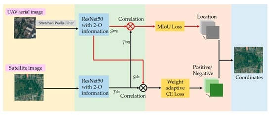
2.2. M-O SiamRPN with Weight Adaptive Joint Multiple Intersection over Union for Visual Localization

Visual localization is accomplished by comparing real-time aerial imagery with pre-stored satellite images, matching the most similar region in the satellite image to the target, and marking the coordinate position. Considering the non-ideal effects of small target size, blurred edges, and non-balanced information in aerial images, we propose an M-O SiamRPN and a weight adaptive joint multiple intersection over union loss function. The former is designed to address the localization task as a classification and detection problem in satellite maps using real-time aerial images as a template through a SiamRPN backbone, where multi-order with multi-resolution features is used to improve the expression ability and sensitivity to edge textures. The latter balances the effectiveness of a large number of negative samples and a small number of positive samples by simultaneously constraining the anchor box with weight adaptive scale and multiple intersection over union.

2.2.1. M-O SiamRPN Framework

As shown in Figure 2, the proposed M-O SiamRPN consists of three critical components: (1) Siamese ResNet backbone for feature extraction applied to the classification branch and regression branch; (2) Multiple-order information generation module based on selected first-order features; (3) Region proposal network (RPN) under multiple constraints:

• Siamese ResNet backbone: Inspired by SiamRPN, the first-order features used for classification and regression to perform correlation are extracted by the Siamese structure of shared weights. Here, to enhance the feature representation, AlexNet is replaced with Resnet50 [22] in the original SiamRPN structure to increase the network depth.
• Multiple-order information generation module is constructed to sufficiently exploit the complementary characteristics of texture sensitivity of second-order information with the semantic information of first-order features and the different resolution features. For further increasing the representation of second-order features for texture, as well as removing redundant information to avoid overly complex networks, a convolution kernel selection criterion based on spatial continuity is proposed. Using this criterion, first-order features with richer texture information are selected for the generation of second-order information. The second-order information is introduced by adding the covariance matrix to the residual module.
• RPN with multiple constraints: Corresponding to the Siamese structure used for feature extraction, RPN also contains two branches: the classification branch and the regression branch, where both branches are performed with correlation operations as:

$$Co{r}^{\mathrm{c}\mathrm{l}\mathrm{s}}=T^{\mathrm{c}\mathrm{l}\mathrm{s}}\otimes S^{\mathrm{c}\mathrm{l}\mathrm{s}}$$

(9)

$$Co{r}^{\mathrm{r}\mathrm{e}\mathrm{g}}=T^{\mathrm{r}\mathrm{e}\mathrm{g}}\otimes S^{\mathrm{r}\mathrm{e}\mathrm{g}}$$

(10)

where Cor^cls and Cor^reg denote the correlation calculation of the classification branch and regression branch, T^cls and T^reg represent the features that the template branch fed into RPN for classification and regression, S^cls and S^reg are search branch features fed into RPN for classification and regression, and ⊗ is correlation calculation. The RPN outputs the location and category scores of the targets through different anchor boxes sliding the features input into the two branches. In the above regression procedure, a weight adaptive joint multiple intersection over union loss function is proposed to optimize the framework, where the weight adaptive scale aims to balance the information between positive and negative samples, and multiple intersection over union is used to improve the accuracy of anchor boxes regression.

2.2.2. First-Order Feature Selection Criteria Based on Spatially Continuity

The essence of convolution is to extract the efficient information of samples with kernels, so the corresponding important feature can be selected through the reasonable judgment of convolution kernels. In practical image processing, the large contiguous region extracted by the convolution kernel represents the corresponding feature maps with large blocks of contiguous pixels, which means that the feature map retains more essential information. Attributed to the different emphases of the features extracted by the kernels with different parameters, the spatial information contained in the convolutional kernel weights is the key to texture and edge extraction.

Here, we propose the concept of spatial continuity of convolutional kernels to integrate the originally scattered spatial information in the kernels, using the spatial information extraction ability as measurement criteria. The spatial continuity coefficient is calculated quantitatively and used to rank the convolution kernels, selecting the feature map with richer spatial information, as shown in Figure 3. For convolutional layers close to the input, this means that the top-ranked feature maps extract more sufficient local information, as shown in Figure 4.

The quantitative calculation of spatial continuity includes connected component analysis and weight information content. It is mathematically described as the sum of the products of the connected areas of all connected domains and the Frobenius norm [33] of the corresponding connected blocks in the matrix, and can be written as:

$$SC={\displaystyle \sum _{k=1}^m{C}_k{\Vert W\Vert }_F}, (x,y)\in A_k$$

(11)

$${\Vert W\Vert }_F=\sqrt{Tr(W^{\mathrm{T}}W)}=\sqrt{{\displaystyle \sum W_{x,y}^2}}$$

(12)

where W is the weight matrix corresponding to the convolution kernel, m is the total number of connected blocks in W, A_k is the kth connected block of W, and C_k is the area of the A_k.

The connected domain is an effective analysis tool in the fields of pattern recognition and image segmentation, which mainly consists of four-neighborhood and eight-neighborhood domains, as shown in Figure 5. Here we choose the eight-neighborhood domain. To obtain the connected domain area C_k, the binarized weight matrix M firstly needs to be calculated:

$$M_{x,y}=\{\begin{array}{c}1, \left|W_{x,y}\right|>\mathrm{threshold} \mathrm{value}\\ 0, \left|W_{x,y}\right|<\mathrm{threshold} \mathrm{value}\end{array}$$

(13)

Here, the threshold value is the hyperparameter. After calculating the M matrix, all the eight-connected domains in the matrix are traversed, and the connected areas of all the eight-connected domains are calculated at the same time. The exploration directions and location during the search process are defined as:

$$directions=[[1,1],[-1,0],[-1,1],[0,-1],[0,1],[1,-1],[1,0],[1,1]]$$

(14)

$$\{\begin{array}{c}{x}^{\prime }=x+directions[k][0]\\ y^{\prime }=y+directions[k][0]\end{array}, 0\le k\le 8$$

(15)

where directions denotes the array of searching directions, x and y are the horizontal and vertical coordinates of the current position, and x′, y′ are next position coordinates to be explored. The visited elements larger than the threshold are added to the connected block, and then the elements linked to the connected block continue to be explored. The total number of elements larger than the threshold that has been explored is the area of the concatenated domain C_k.

Finally, each convolutional kernel is sorted according to the value of spatial continuity, and the corresponding features are selected according to the selection proportion p. In the M-O SiamRPN framework, the first block in ResNet50 is chosen as a candidate to ensure that the features retain sufficient local information, which is conducive to the representation of texture by second-order features. Meanwhile, to combine the simplicity of the framework, p is set to 30% after several experiments, i.e., the features corresponding to the top 30% of the SC ranked convolutional kernels are selected.

2.2.3. Multiple-Order Feature for Blurred Edges of Tiny Target

The backbone of SiamRPN is replaced with a ResNet50, which increases the network depth and improves the semantic representation of the features, but it is still essentially a first-order feature. For the description of blurred edges of tiny targets, the assistance of second-order features is required [34]. The second-order information based on normalized covariance is added to the residual block as an embedded injection layer, shown in Figure 6b. The first-order features applied to produce the second-order information are selected by the SC proposed in Section 2.2.2. This subsection focuses on the generation of second-order information with normalized covariance and the fusion of multi-order features.

After a pair of samples is fed into the Siamese frame, a set of first-order features, i.e., f^1-O ∈ h × w × c, is obtained after extraction and SC selection. f^1-O can be rewritten in vector form according to the same position of different channels as f^1-O = X = {X₁, X₁,…, X_n}, then its corresponding covariance matrix f^2-O is calculated as:

$$f^{2\text{-}\mathrm{O}}=\frac{1}{n}({\displaystyle \sum _{i=1}^{n}X{X}^{\mathrm{T}}})+\epsilon I$$

(16)

$$X{X}^{\mathrm{T}}=\left(\begin{array}{cccc}\mathrm{cov}(X_1,X_1)& \mathrm{cov}(X_1,X_2)& \cdots & \mathrm{cov}(X_1,X_n)\\ \mathrm{cov}(X_1,X_1)& \mathrm{cov}(X_2,X_2)& \cdots & \mathrm{cov}(X_2,X_n)\\ ⋮& ⋮& \ddots & ⋮\\ \mathrm{cov}(X_n,X_1)& \mathrm{cov}(X_n,X_2)& \cdots & \mathrm{cov}(X_n,X_n)\end{array}\right)$$

(17)

$$\mathrm{cov}(X,Y)=E[(X-\overline{X})(Y-\overline{Y})]$$

(18)

where I is the unit matrix, ε denotes a small positive number, cov represents the covariance calculation, and E(•) is the mean value. The second-order covariance with channel interactions is obtained by transposed outer product calculations, whose powerful mathematical statistical guarantees are verified in various classification applications. The vector used to calculate the covariance contains descriptions of different channels for the same location, as shown in Figure 7. Therefore, the obtained second-order information simultaneously yields the higher-order characteristics and the channel complementary [35]. Different from other second-order methods, feature maps with high spatial continuity are selected for conducting second-order calculations, which do not involve dimensional surges and do not require an additional dimensionality reduction step.

The resulting second-order f^2-O belongs to Riemann flow and cannot be directly fused, which needs to be decomposed into Euclidean space [36]. So, the f^2-O is normalized based on eigenvalue decomposition, as shown in Figure 7. Since the covariance matrix f^2-O is the symmetric and positive definite, it can be decomposed by the singular value decomposition (SVD) as:

$$f^{2\text{-}\mathrm{O}}=U\Lambda U^{\mathrm{T}}$$

(19)

where Λ = (λ₁, λ₂,…λ_n) is the diagonal matrix consisting of the eigenvalues λ_n and U = [u₁, u₁,…, u_n] denotes the corresponding eigenvector. It can be seen from Equation (19) that the power normalization processing of covariance matrix f^2-O can be expressed as the power operation of eigenvalue:

$${(f^{2\text{-}\mathrm{O}})}^{\omega }=U{\Lambda }^{\omega }{U}^{\mathrm{T}}$$

(20)

When ω = 0.5, it is the square-root normalization of the matrix. Due to the slow computational speed of GPU for matrix decomposition, the iterative method to calculate the square root is employed to meet the demand for high real-time performance of localization. Let the f^2-O = Z², for the equation:

$$F(Z)=Z^2-f^{2\text{-}\mathrm{O}}=0$$

(21)

Denman-Beavers [37] formula is applied to the iterative solution, avoiding the drawbacks of the pathological case of SVD and poor support on the GPU. The mathematical definition of Denman-Beavers is:

$$K_{k+1}=\frac{1}{2}(K_k+O_k^{-1})$$

(22)

$$O_{k+1}=\frac{1}{2}(O_k+K_k^{-1})$$

(23)

where the initial K₀ is set to f^2-O, O₀ is the unit array I, and K_k and O_k are converged globally at (f^2-O)^1/2 and (f^2-O)^−1/2, respectively. Fifteen iterations have been experimentally demonstrated to be sufficient.

As an injection layer in the residual block, the second-order information based on normalized covariance is segmentally differentiable, which is able to be trained end-to-end by back-propagation. From the chain rule, the partial derivative of the loss function L with respect to f^2-O can be described as:

$$\frac{\partial L}{\partial f^{2\text{-}\mathrm{O}}}=U\{(Q^{\mathrm{T}}\odot (U^{\mathrm{T}}\frac{\partial L}{\partial U}))+{(\frac{\partial L}{\partial \Lambda })}_{diag}\}{U}^{\mathrm{T}}$$

(24)

where the Q is interleaved matrix consisting of elements q as:

$$q_{ij}=\{\begin{array}{l}1/({\lambda }_i-{\lambda }_j),i\ne j\hfill \\ 0,i=j\hfill \end{array}$$

(25)

From the combination of the above equations, the different partial derivatives are obtained as:

$$\frac{\partial L}{\partial U}=\{\frac{\partial L}{\partial Z}+{(\frac{\partial L}{\partial Z})}^{\mathrm{T}}\}U\Lambda$$

(26)

$$\frac{\partial L}{\partial \Lambda }={(\Lambda )}^{\prime }{U}^{\mathrm{T}}\frac{\partial L}{\partial Z}U$$

(27)

$${(\Lambda )}^{\prime }=diag(\frac{1}{2\sqrt{{\lambda }_1}},\frac{1}{2\sqrt{{\lambda }_2}},\dots ,\frac{1}{2\sqrt{{\lambda }_n}})$$

(28)

In a similar manner to the summation of features in the residual module, second-order features are fused by summing matrix elements after channel adjustment:

$$f^{\mathrm{M}\text{-}\mathrm{O}}(x)=f^{1\text{-}\mathrm{O}}(x)\oplus x\oplus f^{2\text{-}\mathrm{O}}$$

(29)

where x denotes the input of the current module, ⊕ is the sum of matrix elements, and element alignment by convolution is omitted here. With the nonlinearity appearing throughout the R² space, the output of the overall network is further increased by adding second-order information to enhance the expression of textures and edges.

2.2.4. Weight Adaptive Joint Multiple Intersection over Union Loss Function

During the training process, only anchor frame coverage exceeding the threshold is determined as a positive sample, while all other cases are negative samples. This setting leads to an imbalanced proportion of positive and negative samples [38]. In an attempt to improve the overall classification performance, the classifier tends to focus less on the minority class and favor the majority class, resulting in the minority samples being difficult to be recognized [39]. In addition, the fast and accurate location regression of the anchor box is also crucial to improving network optimization.

The loss function L of the framework based on SiamRPN consists of two parts, one of which is classification loss L_cls represented by cross-entropy loss and the other is loss function L_reg used to optimize the target position. Therefore, we redesign the loss function for each of the two branches of classification and regression, and the weight adaptive joint multiple intersection over union loss function is proposed to cope with the issue of imbalanced sample information.

For classification loss L_cls, the classical binary cross-entropy loss function is expressed as:

$$L_{\mathrm{CE}}(y_i,p_i)=-(y_i\cdot \log (p_i)+(1-y_i)\cdot \log (1-p_i))$$

(30)

where y_i is the label of the sample x_i and p_i is the output probability. The errors are accumulated equally for each sample, without considering the effect of the majority of negative sample information on the training process. According to the cost-sensitive principle, the penalty weight of minority category samples is additionally increased to enhance the focus on positive samples, improving the identification efficiency of positive samples. Here, a sample mean distribution coefficient AG is defined as:

$$AG=S_{\mathrm{all}}/n$$

(31)

where S_all and n are the numbers of sample categories. The implication of AG is the number of samples contained in each category in the ideal case of a uniform sample. Then, a weighting scale r is defined:

$$r=AG/n_c$$

(32)

where the n_c denotes the number of samples actually classified into category c. For negative samples, the number of samples within the category is larger than AG, so the scale r is less than 1, which serves to reduce the weights. On the contrary, in the case of positive samples, whose number is less than AG, the scale r is greater than 1 and the weight is increased. The scaling of the weights is automatically adapted to the imbalance of the sample categories. By adding the weight adaptive scale r to L_ce, the new loss function of the classification branch is:

$$L_{\mathrm{cls}}=-\frac{1}{N}{\displaystyle \sum _{i=1}^N{r}_i[y_i\log (p_i)+(1-y_i)\log (1-p_i)]}$$

(33)

Deriving the above Equation (34), the gradient is obtained as:

$$g=r_i[y_i\cdot (p_i-1)+(1-y_i)\cdot p_i]$$

(34)

It can be seen that the gradient values are scaled up when the samples are positive, so that the total gradient contribution of both categories to the model optimization process is balanced.

The second part of the loss function is L_reg for predicting the position of the target. Smooth-l₁ is used in SiamRPN for regression optimization, but the four important vertices of the anchor boxes are not included in the optimization metric, which is less robust to rotations, scale changes, and non-overlapping boundaries. The intersection over union (IoU) [25] focuses on the overlap between the prediction anchor box and the groundtruth, considering the whole process as a regression calculation, which is essentially the cross-entropy of the overlap rate:

$$IoU=\frac{S_1\cap S_2}{S_1\cup S_2}$$

(35)

$$L_{IoU}=-p\ln (IoU)-(1-p)\ln (1-IoU)$$

(36)

where S₁ and S₂ are prediction box and groundtruth, respectively, p is the corresponding probability. IoU indicates the overlapping relationship of two borders, which obviously ranges from 0 to 1. However, the case of non-overlapping is not captured by the IoU. In this work, multiple intersection over union (MIoU) is proposed to optimize the regression of the prediction anchor box, designing a more complete loss function, which contains generalized intersection over union (GIoU) and distance intersection over union (DIoU) [40,41].

The non-overlapping part of the two boxes is the concern of the GIoU, aiming to make the two boxes infinitely close from the perspective of minimizing the non-overlapping area, as shown in Figure 8b. Firstly, it is necessary to find the smallest box S₃ that completely wraps S₁ and S₂, and then the area not occupied by the two boxes in S₃ is calculated as:

$$GIoU=IoU-\frac{\left|S_3-(S_1\cup S_2)\right|}{S_3}$$

(37)

$$L_{GIoU}=1-IoU+\frac{\left|S_3-(S_1\cup S_2)\right|}{S_3}$$

(38)

Obviously, when the prediction box S₁ and the groundtruth S₂ do not overlap, i.e., IoU = 0, the value of GIoU is not zero, ensuring that the gradient of the loss function can be propagated backwards. However, when S₁ contains S₂, GIoU degenerates to IoU and the exact regression calculation cannot be implemented through both GIoU and IoU. Therefore, DIoU is introduced and its visualization is shown in Figure 8c. Constraints on the distance between the centers of the two boxes S₁ and S₂ are incorporated in the regression process through DIoU to better characterize the overlap information, which is calculated as:

$$DIoU=IoU-\frac{d(S_1,S_2)}{R(S3)}$$

(39)

$$L_{DIoU}=1-IoU+\frac{d(S_1,S_2)}{R(S_3)}$$

(40)

where d(S₁, S₂) denotes the distance between the centroids of the two boxes and R is the diagonal S₃. Thus, the regression loss function L_reg based on MIoU is a combination of DIoU of GIoU:

$$L_{\mathrm{reg}}=\alpha (1-IoU+\frac{\left|S_3-(S_1\cup S_2)\right|}{S_3})+\beta (1-IoU+\frac{d(S_1,S_2)}{R(S_3)})$$

(41)

where α and β are hyperparameters. The loss function of the overall framework L can be expressed as:

$$Loss=L_{\mathrm{cls}}+L_{\mathrm{reg}}$$

(42)

$$Loss=\frac{1}{n}{\displaystyle \sum _{i=1}^{n}L(y_i,p_i)+}\alpha (1-IoU+\frac{\left|S_3-(S_1\cup S_2)\right|}{S_3})+\beta (1-IoU+\frac{d(S_1,S_2)}{R(S_3)})$$

(43)

2.3. Experiment Setup

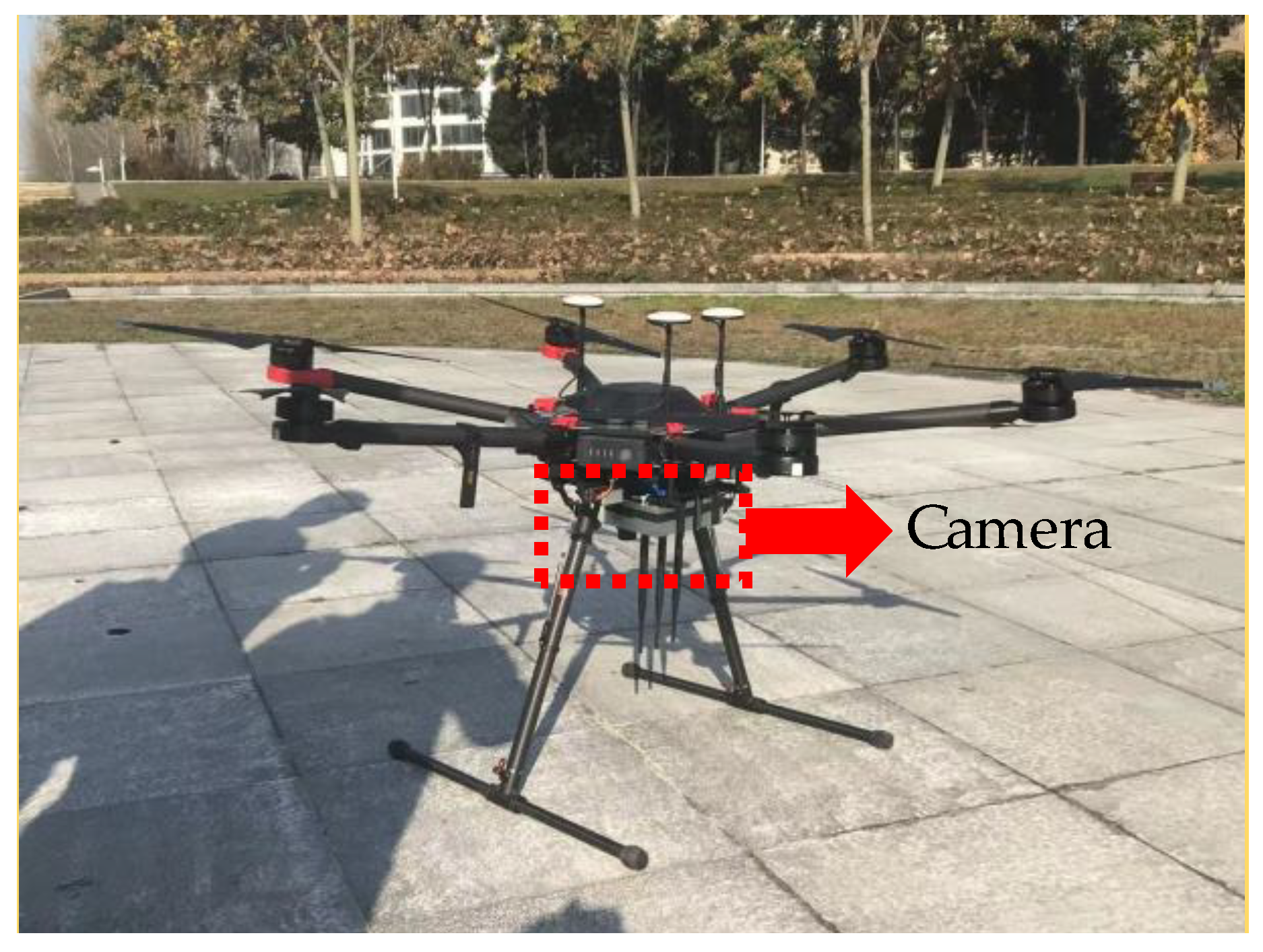
2.3.1. Details about UAV Platform

The experimental platform is based on a DJI M600 UAV and a homemade camera based on an Imx327 sensor with a resolution of 1080P and a frame rate of 60. The UAV platform is shown in Figure 9.

2.3.2. Dataset

The dataset is divided into two parts: aerial images and satellite maps. The aerial images are collected by the self-built UAV platform mentioned above, with a total of 3960 images. The number of aerial images is then expanded to 10,000 by data enhancement processes including panning, zooming, blurring, and flipping, which cover categories such as mountains, forests, rivers, lakes, coastlines, urban intersections, playgrounds, factory buildings, single-family buildings, neighborhood buildings, viaducts, parks, roads without green belts, roads with green belts, etc. Satellite images corresponding to the aerial images are taken from publicly available satellite images.

2.3.3. Network Parameters

Inspired by SiamRPN++ [42], the stride of Stage3 and Stage4 of the backbone ResNet50 are halved and combined with null convolution. The dimensions of the features input to the RPN head for interaction are 25 × 25 and 25 × 25, as illustrated in Figure 2. The threshold of IoU is set to 0.75, which is attributed to the fact that the final output is the location rather than the proposed region.

The proposed framework is constructed on PyTorch with an epoch of 50 and batch size of 128, and the framework is optimized by SGD with a momentum factor of 0.9 and weight decay of 0.0001. The learning rate is increased from 0.005 to 0.01 using Warmup in the first 5 epochs, after which the learning rate decayed from 0.01 to 0.005 in exponential form. The backbone is not trained for the first 10 epochs and the whole framework is trained after the 10th epoch. The hardware platforms used for the experiments are Intel-Core i7-8700K [email protected] and NVIDIA GeForce RTX3090 GPU.

2.3.4. Evaluation Metrics

Reasonable evaluation metrics are an important task for UAV localization. Precision, success rate, frames per second (FPS), and center location error (CLE) are chosen to demonstrate the performance of M-O SiamRPN with multi-optimization loss function.

3. Results

3.1. Training Process Results

During the experiment, we recorded the performance of the M-O SiamRPN with a multi-optimization loss function. The losses in the training process are illustrated in Figure 10. Obviously, the loss decreased rapidly within 10 epochs and leveled off after the 15th epoch. It can be observed that the proposed framework did not suffer from underfitting and overfitting problems, which indicates that our dataset is reasonable and the proposed model is matched to the dataset.

3.2. Performance Evaluation

To fairly validate the proposed framework, comprehensive comparison experiments are conducted. Siamese structure networks similar to our approach i.e., SiamFC [18], SiamRPN [24], SiamRPN++ [42], and other current best performing localization networks such as CFNet [43] and Global Tracker [44]. Here, we record the precision and success rate of all the matching networks, and the details of the different comparison results in different networks are given below. From Figure 11, it is obvious that the M-O SiamRPN with multi-optimization achieved significantly higher precision and success rate than those of other frameworks improving 0.016 and 0.019 over the previous best result of SiamRPN++. The results indicate that the multi-order features proposed in this work enhance the texture representation as well as the weight adaptive multiple optimization being able to reduce the influence of non-equilibrium information.

The performance improvement of the network is usually accompanied by an increase in time complexity. However, for a UAV visual localization task with a high real-time requirement, the framework must complete inference quickly to guarantee localization timeliness. Here, we compare the FPS and CLE of different localization frameworks to verify the processing speed and robustness, and the results are shown in

Table 1. The FPS and CLE of different localization frameworks.

Method	FPS	CLE
This work	35	5.47
SiamRPN++ [42]	30	5.98
SiamRPN [24]	37	6.26
CFNet [43]	47	6.11
SiamFC [18]	41	6.56
Global Tacker [44]	40	5.83

. Since the proposed spatial continuity criterion is effective to select a small amount of significant first-order features, the processing time of M-O SiamRPN with multi-optimization is not remarkably increased even with the additional injection of second-order information. Compared to the structurally similar SiamRPN, our method is slightly slower, which is attributed to the replacement of the first-order feature extraction network and the generation of second-order information. In the proposed framework, 35 frames are processed per second, which is faster than the SiamRPN++ with the same backbone ResNet50.

3.3. Contribution of Multiple-Order Feature

To illustrate the contribution of multiple-order features to promote performance, we compare the AlexNet and ResNet, which are the backbone in SiamRPN and SiamRPN++, respectively, with the backbone proposed in this paper. The results are listed in

Table 2. Ablation studies on the backbone of M-O SiamRPN with weight adaptive joint multiple intersection over union loss function.

Backbone	Precision	Success Rate	FPS	CLE
AlexNet [21]	0.951	0.707	38	6.26
ResNet18 [22]	0.954	0.710	37	6.11
ResNet50 [22]	0.959	0.711	37	6.07
ResNet50 with M-O feature (p = 10%)	0.968	0.722	33	5.54
ResNet50 with M-O feature (p = 30%)	0.979	0.732	35	5.47
ResNet50 with M-O feature (p = 50%)	0.980	0.730	32	5.43
ResNet50 with M-O feature (p = 100%)	0.978	0.730	30	5.50

, embedding the above-mentioned backbones in our framework and discussing the percentage of the added second-order information. By comparing the first-order features, it can be seen that as the depth increases, the network feature description capability is improved and ResNet50 achieved better results than AlexNet with a 0.08 and 0.04 improvement in precision and success rate, respectively. With the injection of second-order information, the performance of the network increases significantly. The framework with 30% and 50% second-order features obtained the highest precision of 0.979 and 0.980, an improvement of 0.020 and 0.021 compared to the first-order Resnet50. The multi-order features benefit the localization success rate, which was improved by 0.11 (p = 10%), 0.21 (p = 30%), 0.19 (p = 50%), and 0.19 (p = 100%), respectively, compared with the first-order backbone ResNet50. Considering the processing speed and centering error, p = 30% is used in practical applications.

3.4. Contribution of Weight Adaptive Joint MIoU Loss Function

The uniform metric Average Precision (AP) is chosen for performance measurement in order to demonstrate in detail the role of weight adaption and multiple intersection over union. AP is the area under the curve of precision versus recall, which is a widely accepted criterion for target detection tasks. We set different IoU thresholds, i.e., IoU = {0.5, 0.6, 0.7, 0.8, 0.9} and used IoU, DIoU, and GIoU as comparisons. The results are reported in

Table 3. Quantitative comparison of M-O SiamRPN using L_IoU, L_CIoU, L_DIoU, L_GIoU, L_MIoU.

Loss Function	AP50	AP60	AP70	AP80	AP90
LIoU	82.46%	72.75%	60.26%	39.57%	8.75%
Relative improve	3.96%	4.70%	3.87%	3.09%	5.12%
LCIoU	83.31%	74.19%	60.71%	39.15%	8.62%
Relative improve	3.11%	3.26%	3.42%	3.51%	5.25%
LDIoU	83.57%	75.14%	61.43%	40.60%	8.81%
Relative improve	2.85%	2.31%	2.70%	2.06%	5.06%
LGIoU	84.18%	76.33%	61.87%	39.64%	9.22%
Relative improve	2.24%	1.12%	2.26%	3.02%	4.65%
LMIoU	85.36%	76.57%	62.61%	40.15%	9.81%
Relative improve.	1.06	0.88%	1.52 %	2.51%	4.06%
LMIoU with weight adaptive	86.42%	77.45%	64.13%	42.66%	13.87%

. L_MIoU with weight adaptive gained the highest AP and L_MIoU achieved the second-best results for all different thresholds of IoU. In addition, L_MIoU with weight adaptive showed the most significant improvement under the harsher conditions with higher thresholds.

3.5. Qualitative Evaluation

The qualitative results of the M-O SiamRPN with multi-optimization and state-of-the-art methods are compared in Figure 12. The left column shows pairs that were correctly localized by all frameworks, and the right column shows pairs that were successfully localized by M-O SiamRPN with multi-optimization but failed to be localized by other frameworks. It can be seen that all methods perform well when obvious features (e.g., bright colors, special edges) appear in the image. In contrast, when the target in the search image is blurred or has similar contours to the surroundings, other localization methods are prone to mislocalization or missed detection, while our framework can still localize correctly. The improvement in localization performance can be attributed to the following aspects. Firstly, the fusion of the second-order covariance information enables the backbone CNN to extract the target features more effectively and characterize the blurred edges more adequately. Secondly, the negative impact of information imbalance on the classifier is reduced due to the integration of weight adaptive scale into the classification branch loss function. Finally, the intersection over union constrains the anchor boxes from different aspects, resulting in more accurate localization of the location regression branches.

4. Discussion

Autonomous high-precision real-time localization in the case of GNSS and other navigation module failures is extremely important for the safe and full-scene application of UAVs. By matching aerial images with satellite maps, vision-based UAV localization can acquire precise coordinates without additional auxiliary information. However, the real-time collected aerial images are limited by non-ideal effects such as shadow occlusion, few pixels occupied by the target to be matched, and blurred edges caused by flight jitter, resulting in vision-based localization that is still challenging. The experimental results show that the M-O SiamRPN with weight adaptive joint multiple intersection over union loss can achieve accurate pure visual localization with an accuracy of 0.974 and a success rate of 0.732.

ResNet50 embedded with second-order information as the backbone of feature extraction can significantly improve the feature representation of the framework. The increase in precision and success rate can be attributed to two aspects: (1) edges are essentially mutations of pixels, and second-order information is more sensitive to mutations. This is consistent with the effectiveness of second-order pooling [45] and second-order features in bilinear CNN [46] in fine-grained classification. In addition, the proposed spatial continuity as an evaluation criterion for first-order features can select feature maps that retain more adequate local information. (2) The fusion of multi-order features enhances the overall nonlinearity of the neural network at the feature map level, enabling better performance of network fitting. In the optimization phase of the framework, we designed a new loss function to address the sample imbalance problem. For the classification branch of the Siamese frame, the penalty coefficient of cross-loss is automatically adjusted to increase the contribution of a few samples to the loss by comparing the distribution of positive samples within the batch to the ideal equilibrium distribution. In the regression branch, the performance of the prediction box and groundtruth box inclusion, as well as non-overlapping cases, is improved by constraining from both the non-overlapping area and the diagonal of the anchor boxes.

Although the proposed model has proven to be accurate and efficient, it does have limitations. By analyzing the failure samples, the precision and success rate of localization are lower in densely vegetated mountainous areas. This is due to the small spacing and dense canopy in mountainous and forested areas, where even different tree species have similar canopy shapes and colors. In addition, the different slopes of the terrain are not clearly reflected in the aerial images due to the absence of other significant references, further increasing the difficulty of localization. Currently, UAV vision provides mainly visible images. In some special applications, it can be supplemented with information from other wavelength bands, such as adding multispectral through hyperspectral cameras. With other spectral information, the UAV obtains both flight altitude and terrain slope features in visual localization, enriching the information contained in aerial images in complex environments. Among them, the reconstruction of targets by multispectral information and the effective fusion of multi-source features will be worth further investigation.

5. Conclusions

In this paper, we focus on the challenge of a tiny target and blured edge detection problem in UAV visual localization. M-O SiamRPN with weight adaptive joint multiple intersection over union loss and a stretched Wallis shadow compensation method are proposed. The pre-processed aerial images significantly reduce the effect of shadows and are the basis for subsequent image matching procedures. M-O SiamRPN with weight adaptive joint multiple intersection over union loss consists of three parts: a dual-stream Siamese first-order framework based on ResNet50; a covariance-based second-order information generation module; and an RPN module under weight adaptive multiple constraints. To exploit the first-order features adequately, we used Resnet50 as the backbone and proposed the concept of spatial continuity to rank the convolution kernels and select the features with richer local information for 2-O feature generation. For the blurred edges of tiny targets, we presented M-O features, which incorporate second-order information obtained by normalized covariance calculation of selected 1-O features to enhance the network description capability. To address the problem of positive and negative sample imbalance in the detection task, a weight adaptive cross-entropy loss and MIoU were designed to improve the regression precision. The former automatically adjusts the penalty coefficient of the loss function according to the number of positive and negative samples, while the latter constrains the interest anchor box from multiple perspectives. We built a consumer-grade UAV acquisition platform to construct an aerial image dataset for experimental validation. The results show that our framework obtained excellent performance for each quantitative and qualitative metric.

The proposed visual framework is only based on a UAV platform, which is capable of autonomously achieving high-precision real-time localization in the event of GNSS and other navigation module failure. This provides the basis for higher-level extended functionality, which is important for safe, full-scene applications of UAVs.

References

1. Li, W.; Li, H.; Wu, Q.; Chen, X.; Ngan, K.N. Simultaneously detecting and counting dense vehicles from drone images. IEEE Trans. Ind. Electron. 2019, 66, 9651–9662. [Google Scholar] [CrossRef]
2. Ye, Z.; Wei, J.; Lin, Y.; Guo, Q.; Zhang, J.; Zhang, H.; Deng, H.; Yang, K. Extraction of Olive Crown Based on UAV Visible Images and the U2-Net Deep Learning Model. Remote Sens. 2022, 14, 1523. [Google Scholar] [CrossRef]
3. Workman, S.; Souvenir, R.; Jacobs, N. Wide-Area Image Geolocalization with Aerial Reference Imagery. In Proceedings of the IEEE International Conference on Computer Vision (ICCV), Santiago, Chile, 7–13 December 2015; pp. 3961–3969. [Google Scholar]
4. Morales, J.J.; Kassas, Z.M. Tightly Coupled Inertial Navigation System with Signals of Opportunity Aiding. IEEE Trans. Aerosp. Electron. Syst. 2021, 57, 1930–1948. [Google Scholar] [CrossRef]
5. Zhang, F.; Shan, B.; Wang, Y.; Hu, Y.; Teng, H. MIMU/GPS Integrated Navigation Filtering Algorithm under the Condition of Satellite Missing. In Proceedings of the IEEE CSAA Guidance, Navigation and Control Conference (GNCC), Xiamen, China, 10–12 August 2018. [Google Scholar]
6. Liu, Y.; Luo, Q.; Zhou, Y. Deep Learning-Enabled Fusion to Bridge GPS Outages for INS/GPS Integrated Navigation. IEEE Sens. J. 2022, 22, 8974–8985. [Google Scholar] [CrossRef]
7. Guo, Y.; Wu, M.; Tang, K.; Tie, J.; Li, X. Covert spoofing algorithm of UAV based on GPS/INS-integrated navigation. IEEE Trans. Veh. Technol. 2019, 68, 6557–6564. [Google Scholar] [CrossRef]
8. Wortsman, M.; Ehsani, K.; Rastegari, M.; Farhadi, A.; Mottaghi, R. Learning to Learn How to Learn: Self-Adaptive Visual Navigation Using Meta-Learning. In Proceedings of the IEEE/CVF Conference on Computer Vision and Pattern Recognition (CVPR), Long Beach, CA, USA, 15–20 June 2019; pp. 6743–6752. [Google Scholar]
9. Qian, J.; Chen, K.; Chen, Q.; Yang, Y.; Zhang, J.; Chen, S. Robust Visual-Lidar Simultaneous Localization and Mapping System for UAV. IEEE Geosci. Remote Sens. Lett. 2022, 19, 1–5. [Google Scholar] [CrossRef]
10. Zheng, Z.; Wei, Y.; Yang, Y. University-1652: A multi-view multi-source benchmark for drone-based geo-localization. arXiv 2020, arXiv:2002.12186. [Google Scholar]
11. Liu, Y.; Tao, J.; Kong, D.; Zhang, Y.; Li, P. A Visual Compass Based on Point and Line Features for UAV High-Altitude Orientation Estimation. Remote Sens. 2022, 14, 1430. [Google Scholar] [CrossRef]
12. Majdik, A.L.; Verda, D.; Albers-Schoenberg, Y.; Scaramuzza, D. Air-ground matching: Appearance-based gps-denied urban localization of micro aerial vehicles. J. Field Robot. 2015, 32, 1015–1039. [Google Scholar] [CrossRef]
13. Chang, K.; Yan, L. LLNet: A Fusion Classification Network for Land Localization in Real-World Scenarios. Remote Sens. 2022, 14, 1876. [Google Scholar] [CrossRef]
14. Zhai, R.; Yuan, Y. A Method of Vision Aided GNSS Positioning Using Semantic Information in Complex Urban Environment. Remote Sens. 2022, 14, 869. [Google Scholar] [CrossRef]
15. Nassar, A.; Amer, K.; ElHakim, R.; ElHelw, M. A Deep CNN-Based Framework for Enhanced Aerial Imagery Registration with Applications to UAV Geolocalization. In Proceedings of the IEEE/CVF Conference on Computer Vision and Pattern Recognition Workshops (CVPRW), Salt Lake City, UT, USA, 18–22 June 2018; pp. 1513–1523. [Google Scholar]
16. Ahn, S.; Kang, H.; Lee, J. Aerial-Satellite Image Matching Framework for UAV Absolute Visual Localization using Contrastive Learning. In Proceedings of the International Conference on Control, Automation and Systems (ICCAS), Jeju, Korea, 12–15 October 2021. [Google Scholar]
17. Wu, Q.; Xu, K.; Wang, J.; Xu, M.; Manocha, D. Reinforcement learning based visual navigation with information-theoretic regularization. IEEE Robot. Autom. Lett. 2021, 6, 731–738. [Google Scholar] [CrossRef]
18. Cen, M.; Jung, C. Fully Convolutional Siamese Fusion Networks for Object Tracking. In Proceedings of the IEEE International Conference on Image Processing (ICIP), Athens, Greece, 7–10 October 2018; pp. 3718–3722. [Google Scholar]
19. Zhu, Z.; Wang, Q.; Li, B.; Wu, W.; Yan, J.; Hu, W. Distractor-aware Siamese Networks for Visual Object Tracking. In Proceedings of the European Conference on Computer Vision (ECCV), Munich, Germany, 8–14 September 2018. [Google Scholar]
20. He, A.; Luo, C.; Tian, X.; Zeng, W. A Twofold Siamese Network for Real-Time Object Tracking. In Proceedings of the IEEE/CVF Conference on Computer Vision and Pattern Recognition (CVPR), Salt Lake City, UT, USA, 18–23 June 2018; pp. 4834–4843. [Google Scholar]
21. Russakovsky, O.; Deng, J.; Su, H.; Krause, J.; Satheesh, S.; Ma, S. Imagenet large scale visual recognition challenge. Int. J. Comput. Vis. 2015, 115, 211–252. [Google Scholar] [CrossRef]
22. He, K.; Zhang, X.; Ren, S.; Sun, J. Deep residual learning for image recognition. In Proceedings of the IEEE Conference on Computer Vision and Pattern Recognition (CVPR), Las Vegas, NV, USA, 27–30 June 2016; pp. 770–778. [Google Scholar]
23. Huang, G.; Liu, Z.; Laurens, V.; Weinberger, K.Q. Densely Connected Convolutional Networks. In Proceedings of the IEEE Conference on Computer Vision and Pattern Recognition (CVPR), Honolulu, HI, USA, 21–26 July 2017; pp. 2261–2269. [Google Scholar]
24. Li, B.; Yan, J.; Wu, W.; Zhu, Z.; Hu, X. High Performance Visual Tracking with Siamese Region Proposal Network. In Proceedings of the IEEE/CVF Conference on Computer Vision and Pattern Recognition (CVPR), Salt Lake City, UT, USA, 18–23 June 2018; pp. 8971–8980. [Google Scholar]
25. Girshick, R. Fast R-CNN. In Proceedings of the IEEE International Conference on Computer Vision (ICCV), Santiago, Chile, 7–13 December 2015; pp. 1440–1448. [Google Scholar]
26. Jiang, H.; Chen, A.; Wu, Y.; Zhang, C.; Chi, Z.; Li, M.; Wang, X. Vegetation Monitoring for Mountainous Regions Using a New Integrated Topographic Correction (ITC) of the SCS + C Correction and the Shadow-Eliminated Vegetation Index. Remote Sens. 2022, 14, 3073. [Google Scholar] [CrossRef]
27. Chen, J.; Huang, B.; Li, J.; Wang, Y.; Ren, M.; Xu, T. Learning Spatio-Temporal Attention Based Siamese Network for Tracking UAVs in theWild. Remote Sens. 2022, 14, 1797. [Google Scholar] [CrossRef]
28. Yu, W.; Yang, K.; Yao, H.; Sun, X.; Xu, P. Exploiting the complementary strengths of multi-layer CNN features for image retrieval. Neurocomputing 2017, 237, 235–241. [Google Scholar] [CrossRef]
29. Feng, J.; Xu, P.; Pu, S.; Zhao, K.; Zhang, H. Robust Visual Tracking by Embedding Combination and Weighted-Gradient Optimization. Pattern Recognit. 2020, 104, 107339. [Google Scholar] [CrossRef]
30. Zhu, X.X.; Tuia, D.; Mou, L.; Xia, G.S.; Zhang, L.; Xu, F. Deep learning in remote sensing: A comprehensive review and list of resources. IEEE Trans. Geosci. Remote Sens. 2018, 5, 8–36. [Google Scholar] [CrossRef]
31. Gao, X.; Wan, Y.; Zheng, S. Automatic Shadow Detection and Compensation of Aerial Remote Sensing Images. Geomat. Inf. Sci. Wuhan Univ. 2012, 37, 1299–1302. [Google Scholar]
32. Zhou, T.; Fu, H.; Sun, C.; Wang, S. Shadow Detection and Compensation from Remote Sensing Images under Complex Urban Conditions. Remote Sens. 2021, 13, 699. [Google Scholar] [CrossRef]
33. Powell, M. Least frobenius norm updating of quadratic models that satisfy interpolation conditions. Math Program. 2004, 100, 183–215. [Google Scholar] [CrossRef]
34. Gatys, L.A.; Ecker, A.S.; Bethge, M. Image Style Transfer Using Convolutional Neural Networks. In Proceedings of the IEEE Conference on Computer Vision and Pattern Recognition (CVPR), Las Vegas, NV, USA, 27–30 June 2016. [Google Scholar]
35. Wu, Y.; Sun, Q.; Hou, Y.; Zhang, J.; Wei, X. Deep covariance estimation hashing. IEEE Access 2019, 7, 113225. [Google Scholar] [CrossRef]
36. Li, P.; Chen, S. Gaussian process approach for metric learning. Pattern Recognit. 2019, 87, 17–28. [Google Scholar] [CrossRef]
37. Denman, E.D.; Beavers, A.N. The matrix Sign function and computations in systems. Appl. Math. Comput. 1976, 2, 63–94. [Google Scholar] [CrossRef]
38. Fan, Q.; Zhuo, W.; Tang, C.K.; Tai, Y.W. Few-Shot Object Detection with Attention-RPN and Multi-Relation Detector. In Proceedings of the IEEE/CVF Conference on Computer Vision and Pattern Recognition (CVPR), Seattle, WA, USA, 13–19 June 2020; pp. 4012–4021. [Google Scholar]
39. Saqlain, M.; Abbas, Q.; Lee, J.Y. A Deep Convolutional Neural Network for Wafer Defect Identification on an Imbalanced Dataset in Semiconductor Manufacturing Processes. IEEE Trans. Semicond. Manuf. 2020, 33, 436–444. [Google Scholar] [CrossRef]
40. Rezatofighi, H.; Tsoi, N.; Gwak, J.Y.; Sadeghian, A.; Reid, I.; Savarese, S. Generalized intersection over union: A metric and a loss for bounding box regression. In Proceedings of the IEEE/CVF Conference on Computer Vision and Pattern Recognition (ICCV), Long Beach, CA, USA, 15–20 June 2019; pp. 658–666. [Google Scholar]
41. Zheng, Z.; Wang, P.; Liu, W.; Li, J.; Ye, R.; Ren, D. Distance-iou loss: Faster and better learning for bounding box regression. arXiv 2019, arXiv:1911.08287. [Google Scholar] [CrossRef]
42. Li, B.; Wu, W.; Wang, Q.; Zhang, F.; Xing, J.; Yan, J. SiamRPN++: Evolution of Siamese Visual Tracking with Very Deep Networks. In Proceedings of the IEEE/CVF Conference on Computer Vision and Pattern Recognition (CVPR), Long Beach, CA, USA, 15–20 June 2019; pp. 4277–4286. [Google Scholar]
43. Shen, Z.; Dai, Y.; Rao, Z. CFNet: Cascade and Fused Cost Volume for Robust Stereo Matching. In Proceedings of the IEEE/CVF Conference on Computer Vision and Pattern Recognition (CVPR), Nashville, TN, USA, 20–25 June 2021; pp. 13901–13910. [Google Scholar]
44. Huang, L.; Zhao, X.; Huang, K. GlobalTrack: A Simple and Strong Baseline for Long-term Tracking. arXiv 2019, arXiv:1912.08531. [Google Scholar] [CrossRef]
45. Li, P.; Xie, J.; Wang, Q.; Zuo, W. Is Second-Order Information Helpful for Large-Scale Visual Recognition? In Proceedings of the IEEE International Conference on Computer Vision (ICCV), Venice, Italy, 22–29 October 2017; pp. 2089–2097. [Google Scholar]
46. Lin, T.-Y.; RoyChowdhury, A.; Maji, S. Bilinear Convolutional Neural Networks for Fine-Grained Visual Recognition. IEEE Trans. Pattern Anal. Mach. Intell. 2018, 40, 1309–1322. [Google Scholar] [CrossRef]
Figure 1. Shadow compensation results using Stretched Wallis.
Remotesensing 14 04467 g001
Figure 2. M-O SiamRPN with weight adaptive joint multiple intersection over union framework.
Remotesensing 14 04467 g002
Figure 3. Schematic of convolutional kernel spatial information ranking.
Remotesensing 14 04467 g003
Figure 4. Convolutional kernels and feature maps arranged by spatial continuity from largest to smallest (9 randomly selected): (a) Input sample; (b) convolutional kernels and the corresponding feature maps.
Remotesensing 14 04467 g004
Figure 5. Diagram of 4-neighborhood and 8-neighborhood: (a) 4-neighborhood; (b) 4-diagonal neighborhood; (c) 8-neighborhood.
Remotesensing 14 04467 g005
Figure 6. Generation of multi-order features in residual blocks: (a) Traditional residual block; (b) proposed multi-information residual block.
Remotesensing 14 04467 g006
Figure 7. The generation of 2-O information based on covariance.
Remotesensing 14 04467 g007
Figure 8. Schematic diagram of different intersection over union: (a) IoU; (b) GIoU; (c) DIoU.
Remotesensing 14 04467 g008
Figure 9. Homemade UAV platform based on DJI M600 and 1080P camera.
Remotesensing 14 04467 g009
Figure 10. Losses of the M-O SiamRPN with multi-optimization: (a) The loss of classification branch; (b) The loss of location regression branch; (c) The total loss.
Remotesensing 14 04467 g010
Figure 11. (a) Precision and (b) success plots of M-O SiamRPN with multi-optimization and state-of-the-art frameworks. The mean precision and AUC scores are reported for each framework.
Remotesensing 14 04467 g011
Figure 12. Qualitative comparison of M-O SiamRPN with multi-optimization and state-of-the-art frameworks.
Remotesensing 14 04467 g012