Abstract
Biomass is a key biophysical parameter for precision agriculture and plant breeding. Fast, accurate and non-destructive monitoring of biomass enables various applications related to crop growth. In this paper, strawberry dry biomass weight was modeled using 4 canopy geometric parameters (area, average height, volume, standard deviation of height) and 25 spectral variables (5 band original reflectance values and 20 vegetation indices (VIs)) extracted from the Unmanned Aerial Vehicle (UAV) multispectral imagery. Six regression techniques—multiple linear regression (MLR), random forest (RF), support vector machine (SVM), multivariate adaptive regression splines (MARS), eXtreme Gradient Boosting (XGBoost) and artificial neural network (ANN)—were employed and evaluated for biomass prediction. The ANN had the highest accuracy in a five-fold cross-validation, with R2 of 0.89~0.93, RMSE of 7.16~8.98 g and MAE of 5.06~6.29 g. As for the other five models, the addition of VIs increased the R2 from 0.77~0.80 to 0.83~0.86, and reduced the RMSE from 8.89~9.58 to 7.35~8.09 g and the MAE from 6.30~6.70 to 5.25~5.47 g, respectively. Red-edge-related VIs, including the normalized difference red-edge index (NDRE), simple ratio vegetation index red-edge (SRRedEdge), modified simple ratio red-edge (MSRRedEdge) and chlorophyll index red and red-edge (CIred&RE), were the most influential VIs for biomass modeling. In conclusion, the combination of canopy geometric parameters and VIs obtained from the UAV imagery was effective for strawberry dry biomass estimation using machine learning models.
1. Introduction
Biomass is a crucial biophysical parameter for precision agriculture and plant breeding. It is the result of photosynthesis [1,2] and other physiological processes involved in the uptake and use of sunlight, water, and mineral nutrients [3]. Biomass measurements allow farmers to assess crop growth status and soil fertility [4] and thus implement efficient management measures, such as the amount and timing of fertilizer, pesticide, and water supply to ensure crop health [5,6]. It is also a key trait measured by plant breeders [7,8]. Thus, rapid, accurate and non-destructive measurements of plant biomass are of great value in various aspects of precision agriculture.
Traditional destructive measurements are time-consuming and labor-intensive [9,10] and cannot assess the biomass of the same plant throughout its growth cycle [11,12]. To solve this problem, studies on the estimation of plant biomass from image-derived parameters are emerging continuously. Satellite-based data have proven effective in predicting and mapping forest and energy crop biomass [13,14,15,16]. Ahmad et al. [17] investigated the application of high-resolution (≤5 m) optical satellite imagery such as QuickBird, WordView-3 and IKONOS for forest above-ground biomass (AGB) estimation. This work demonstrated that using satellite-derived independent variables including tree canopy, image texture, tree shadow fraction, canopy height and vegetation indices (VIs) can yield prediction accuracies (R2) higher than 0.8 in regional-scale studies. Naik et al. [18] compared multi-source multispectral remote sensing data acquired by Sentinel-2 (10 m, 12 bands), RapidEye (5 m, 5 bands) and Dove (3 m, 4 bands) satellites in the prediction task of forest AGB, showing that red-edge and short-wave infrared (SWIR) channel-dependent variables significantly improved the model performance.
Many attempts have also been made to establish the relationship between satellite VIs and the biomass of various crops, such as rice, wheat, and soybeans [19,20,21]. Geng et al. [22] calculated nine VIs from MODIS satellite reflectance data and adopted four machine learning methods, including random forest (RF), support vector machine (SVM), artificial neural network (ANN) and eXtreme Gradient Boosting (XGBoost), to estimate corn biomass, with R2 values between 0.72 and 0.78. Dong et al. [23] extracted multiple red-edge, near-infrared (NIR) and SWIR-based VIs from Landsat 8 and Sentinel-2 satellite data. Statistical approaches (linear and non-linear regressions) were used to obtain the leaf area index (LAI) of six crops (canola, soybean, wheat, corn, oat, and beans). The computed LAI, climate and soil datasets were assimilated to reparametrize a simple crop growth model to estimate the dry biomass of the above crops. The R2 of dry biomass estimation reached 0.8, which is higher than when using only empirical methods between biomass and VIs. The limitation of the satellite VI-based statistical/machine learning methods is that satellite VIs are often affected by the plant growth state and external environmental conditions (e.g., cloud cover), which makes it non-universal for different crops and regions [13,24]. In addition, for precision agriculture at the single plant level, satellite imagery does not have sufficient spatial resolution.
Over the past decade, Unmanned Aerial Vehicles (UAVs) (drones) have emerged as one of the most popular tools for field-based phenotyping and precision agriculture [25,26,27]. They provide a flexible and easy-to-operate approach to collect high spatial (centimeter level) and temporal imagery for high-throughput crop phenotyping [28]. Various types of sensors, including spectral sensors (e.g., RGB, multispectral and hyperspectral cameras) and depth sensors (LiDAR), have been mounted on drones to collect data for crop biomass estimation [10,29]. Correspondingly, image processing technologies have also improved greatly. Photogrammetry software using the Structure in Motion (SfM) method, such as Pix4D and Agisoft Metashape, enables the fast and efficient preprocessing of remote sensing data and generates 3D point clouds and high-quality orthoimages, which provide detailed structural properties of crops [30,31,32].
In recent years, numerous studies have been conducted to monitor crop biomass based on variables (usually crop height, canopy area, textual features, VIs, etc.) obtained from UAV imagery. For example, Fu et al. [33] evaluated the influence of two types of features on the winter wheat biomass predictive performance of partial least squares regression (PLSR) and least squares support vector machine (LSSVM) models. One type of feature was the multiscale texture obtained from UAV-based RGB imagery, and the other comprised various spectral features including the two-band normalized difference vegetation index (NDVI) and continuum removal of red-edge spectra (SpeCR) obtained from ground-based hyperspectral data. The results showed that the combination of SpeCR and multiscale textures achieved the highest estimation accuracy, with R2 = 0.87 and RMSE = 119.76 g/m2. Johansen et al. [34] adopted the RF machine learning approach to predict the biomass of tomato plants based on shape features (plant area, border length, width, etc.), entropy texture and VIs derived from UAV multispectral imagery. The highest explained variances were approximately 87.95%.
Wang et al. [35] estimated the AGB of winter wheat using forty-four VIs extracted from UAV multispectral images. Three methods, including MLR, RF and PLSR, were adopted, and the performance of the RF models was more stable, with R2 ranging from 0.83 to 0.93 in the validation dataset. Some influential VIs include the Modified Chlorophyll Absorption Ratio Index—Improved (MCARI2), Leaf Chlorophyll Index (LCI) and Chlorophyll Vegetation Index (CVI), etc. Che et al. [36] established regression models between the biomass of cultivated red algae Pyropia and four VIs derived from UAV multispectral images. The quadratic model of the difference vegetation index (DVI) showed more accuracy, with R2 of 0.925. Although the VI approach for predicting above-ground biomass suffers from the saturation problem since VIs tend to lose sensitivity as the crop canopy becomes more dense, it remains a popular method for estimating crop biomass. Several studies also demonstrated that multispectral and hyperspectral data with more wavebands have great potential to overcome the saturation problem [37,38].
For cultivated strawberry (Fragaria × ananassa), there are few studies predicting the dry biomass from image-derived parameters. Guan et al. [39] applied the SfM and Object-Based Image Analysis (OBIA) method on very-high-resolution imagery (0.5 mm for raw images) acquired by a tractor-mounted imaging system to extract canopy-related variables such as area, volume, and average height. Multilinear regression was adopted to model the strawberry canopy dry biomass and leaf area, with accuracy (R2) of 0.79 and 0.84, respectively. Abd-Elrahman et al. [40] continued Guan et al. (2020)’s study and proposed a raster-based geospatial analysis method for automatic canopy delineation, size metric extraction and dry biomass prediction using ArcMap software. However, biomass estimation for strawberry using lower-resolution UAV images has not yet been demonstrated. The overall goal of the present study is to apply various machine learning techniques to model strawberry canopy dry biomass from UAV multispectral imagery. The main objectives of this study were to: (1) compare the predictive performance of six regression methods (MLR, RF, SVM, XGBoost, MARS, ANN) in the estimation of strawberry canopy biomass and examine the stability of these models; (2) compare the influence of strawberry canopy structural parameters (canopy area, average height, volume and standard deviation of height) and VIs on models’ performance; and (3) determine the optimal number of features and significant spectral variables (VIs) for strawberry canopy biomass prediction.
2. Materials and Methods
2.1. Study Site and Plant Materials
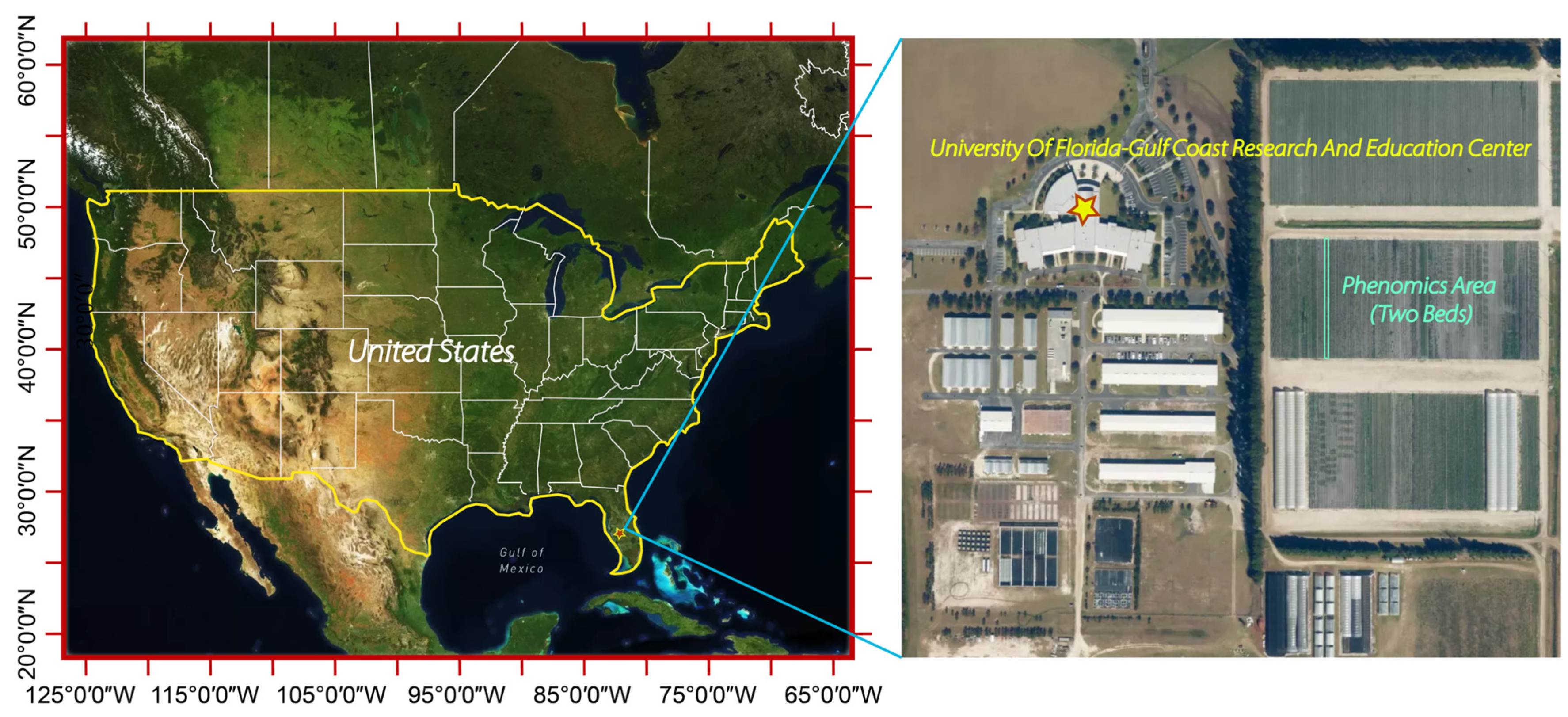
The study area (27°45′40″N, 82°13′40″W) was situated at the University of Florida’s Gulf Coast Research and Education Center (GCREC), located in Wimauma, Florida, USA (Figure 1). We conducted UAV surveys and in-situ biomass measurements during the winter growing season from 19 November 2020 to 3 March 2021. Two 100-m-long beds cultivated with seventeen strawberry genotypes (Table 1) were established. Each bed contained sixteen plots, and each plot was planted with seventeen plants, each corresponding to one of the genotypes tested in this experiment. The genotypes represented the range of canopy structures in the UF strawberry breeding germplasm, as well as varieties with unique canopy structures and sizes from other breeding programs. A code using capital letters (A–Q) was marked on the bed surface near each strawberry plant to indicate its genotype. Approximately every week, two plots were randomly selected, and thirty-four plants were removed to the laboratory for dry biomass measurements. The UAV multispectral imagery was acquired within a few hours prior to plant removal. The plants were placed in a drying oven at 65 °C for 5 days to obtain the dry biomass weight. There was a total of 532 strawberry plant samples in the 2020–2021 season. The detailed information of genotypes and plots is shown in Table 1.
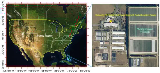
Figure 1.
Study site of the strawberry field at Gulf Coast Research and Education Center of University of Florida.

Table 1.
Statistics of dry biomass of 17 genotypes measured throughout the 2020–2021 growing season using destructive methods.
2.2. UAV Image Acquisition and Ground Control Points (GCP)
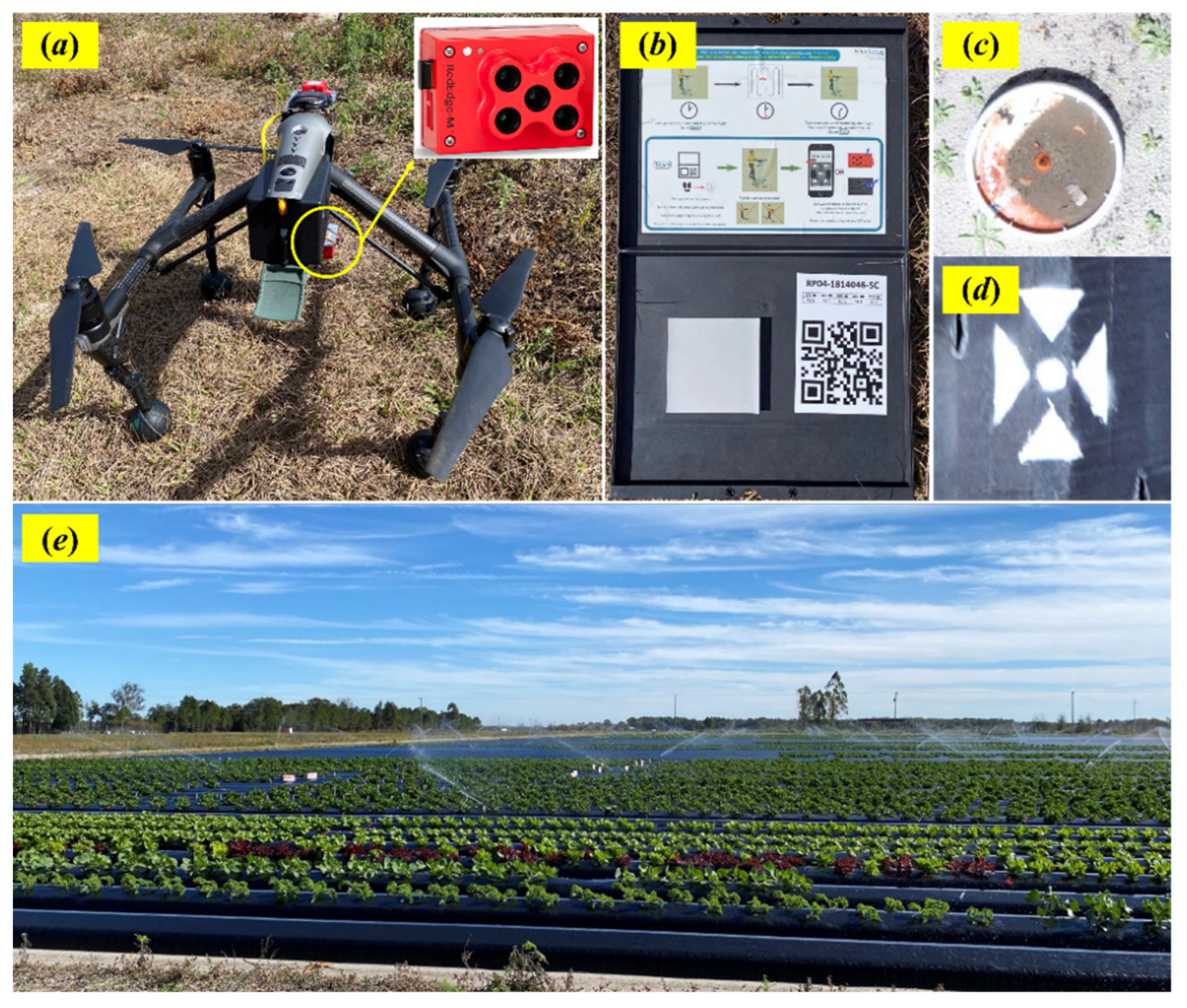
Image acquisition was conducted using a MicaSense RedEdge-M multispectral camera and a downwelling light sensor (DLS) mounted on a Da-Jiang Innovations (DJI) Inspire 2 drone (Figure 2a). The drone operated autonomously, with field flight parameters pre-set using the Litchi flight planning software to cover the whole strawberry experiment area. The UAV flew at an altitude of 15 m above the ground, with a speed of 2 m/s, capturing images with more than 70% overlap and approximately 1-cm raw spatial resolution. The MicaSense multispectral camera contained five spectral bands: blue (475 nm, 20 nm bandwidth), green (560 nm, 20 nm bandwidth), red (668 nm, 10 nm bandwidth), near-infrared (840 nm, 40 nm bandwidth) and red-edge (717 nm, 10 nm bandwidth). The images were captured weekly from 19 November 2020 to 3 March 2021, for a total of 16 collections. The images were captured between 11:00 am and 1:00 pm in as clear and cloudless weather conditions as possible. Before and after each flight, the MicaSense camera was placed above a MicaSense calibrated reflectance panel (Figure 2b) to take white reference images to be used in subsequent image radiometric calibration.

Figure 2.
UAV systems and GCP setup: (a) the Inspire 2 platform equipped with a MicaSense RedEdge-M multispectral camera; (b) the calibration reflectance panel (CRP); (c) GCPs around the strawberry beds (M1–M8); (d) GCPs on the plastic beds (N1–N16); (e) strawberry farm.
Prior to the UAV flight, we established two sets of centimeter-level ground control points (GCPs) in the field to provide accurate image georeferencing and photo alignment during image preprocessing. Two types of control points were established: (1) 8 GCPs (M1–M8) were placed evenly around the field—for each GCP, we used a survey total station to obtain the positional information of these GCPs (Figure 2c); the other GCPs (N1–N16) were distributed evenly on the plastic strawberry beds as redundant points in case other points were destroyed (Figure 2d). This set of GCPs was surveyed using static GNSS observations.
2.3. Ground-Based Image Collection
In addition to UAVs, this study also used a ground-based platform introduced by Abd-Elrahman et al. [41,42] to obtain high spatial resolution (0.5 mm raw images) to evaluate the quality of UAV images (Figure 3). Two Nikon D300 cameras were used to capture RGB and NIR images, respectively. The imaging system was toweled by a tractor in the strawberry field. More detailed information about this platform is presented in Guan et al. [39] and Abd-Elrahman et al. [40]. Three sets of ground-based images were collected on 8 December 2020, 27 January 2021 and 3 March 2021, which roughly reflected the characteristics of strawberry plants in the early, middle, and mature stages. Orthomosaic images (1 mm per pixel) and DSM products (2 mm per pixel) were generated through the SfM analysis in the Agisoft Metashape software. We extracted four strawberry canopy geometric parameters (canopy area, average height, volume, stand deviation of height) from ground-based images and UAV images, and then compared the differences in the two types of image data, as discussed in Section 3.1.
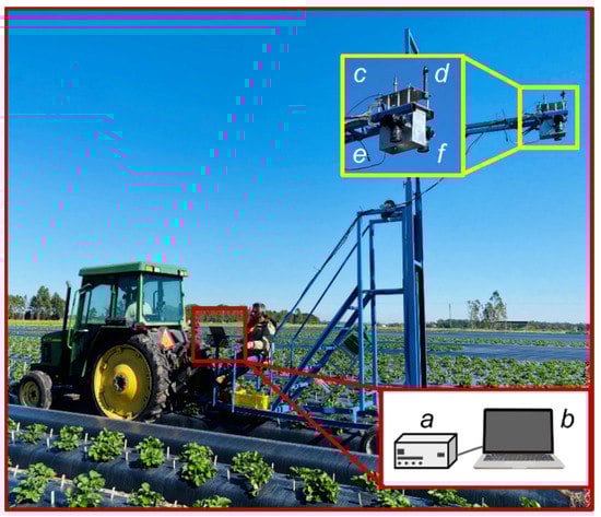
Figure 3.
Ground-based imaging platform pulled by a tractor carrying (a) camera trigger box hardware; (b) computer; (c) timing GPS; (d) GNSS navigation system; (e) Nikon D300 RGB camera and (f) Nikon D300 NIR camera.
2.4. Experimental Workflow
Figure 4 illustrates the workflow adopted in this study, which includes (1) UAV multispectral data preprocessing using the Agisoft Metashape software; (2) strawberry plant canopy delineation and structural metric extraction; (3) calculation of vegetation indices; (4) development and validation of the regression models.
2.4.1. UAV Image Preprocessing Using Agisoft Metashape Software
The multispectral images captured by the MicaSense camera were preprocessed using the Agisoft Metashape Photogrammetry software. Radiometric calibration is crucial to the quality of the surface reflectance image produced by the Agisoft software, which is affected by sensor settings, properties, and scene illumination. A white reference image of the calibrated reflectance panel (CRP), along with panel reflectance values provided by the manufacturer, were imported into the Agisoft software, and the UAV images were converted form raw digital number (DN) to radiance and then from radiance to reflectance for each of the five bands. DLS calibration was only used for the images acquired on 25 November 2020 and 13 January 2021, as both dates were cloudy. Using the Structure from Motion (SfM) algorithm, the Agisoft Metashape combined the images taken from multiple angles and generated dense 3D point clouds of scene objects (strawberry canopies, soils, and beds). A digital surface model (DSM) was created from the SfM-based point cloud, and a georeferenced orthomosaic image was generated for each band. The spatial resolution of both DSM and orthomosaic images had 1-cm pixel size.
2.4.2. Canopy Delineation and Structural Parameter Extraction
A geospatial analysis workflow developed by Abd-Elrahman et al. [40] was used for strawberry canopy delineation. This method was implemented on the ESRI’s ArcMap v10.7 and used the marker-controlled watershed algorithm to extract individual plant boundaries. A vector layer containing a point located at the center of each plant canopy, a vegetation mask obtained from the NDVI using the shadow ratio threshold segmentation method and a DSM produced by the SfM algorithm were imported into the model to iteratively generate boundaries for each strawberry plant in the UAV orthomosaic images. As for the canopy size metric extraction, a vegetation-free digital terrain model (DTM) using the local polynomial interpolation technique was created using the elevations of unvegetated areas. Then, the strawberry canopy height model was computed as the difference between the DSM and DTM to extract the canopy area, volume, average height, and standard deviation of height for each strawberry plant canopy (Figure 4).
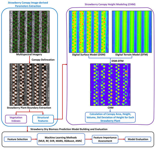
Figure 4.
A workflow diagram showing the methodology adopted in this study, including data preprocessing, feature extraction and biomass predictive modeling.
Figure 4.
A workflow diagram showing the methodology adopted in this study, including data preprocessing, feature extraction and biomass predictive modeling.

2.4.3. Selection of Vegetation Indices
In addition to the surface reflectance values of the five spectral bands, we selected 20 VIs that are commonly used to estimate canopy biophysical parameters, as shown in Table 2. The sum and mean values of all pixels within each plant canopy were calculated for the 20 VIs and 5 individual band values to represent the spectral variables. Therefore, we generated a total of 29 dependent variables (25 spectral features and 4 canopy structural variables) for the biomass modeling.
Table 2.
Vegetation indices (VIs) selected for the biomass estimation. ρRed, ρGreen, ρBlue, ρNIR and ρRedEdge are the reflectance values of the red, green, blue, near-infrared, and red-edge bands.
2.4.4. Biomass Modeling
All modeling was implemented in R Studio 1.4 software using the R programming language (R version 4.0.2). The following six regression techniques were employed in this study.
- (1)
- Multiple linear regression (MLR) is a statistical method that uses several independent variables to predict the outcome of one dependent variable. The regression equation is designed to establish a linear relationship between the response variable with each independent variable and uses the least squares method to calculate the model parameters by minimizing the sum of squared errors [59].
- (2)
- Random forest (RF) is a supervised machine learning algorithm that uses an ensemble learning (bagging) strategy to solve classification and regression problems. Bagging, also referred to as bootstrap aggregation, is a sampling technique that generates a fixed number of subset training samples from the original dataset. The idea of random forest is to build multiple decision trees by selecting a random number of samples and features (bagging) during the training process and output the average prediction of all regression trees.
- (3)
- Support vector machine (SVM) is also a popular machine learning algorithm, widely used in pattern recognition, classification and prediction. There are two types of SVM, support vector classification (SVC) [60] for classification and support vector regression (SVR) [61]. The objective of SVM is to construct a hyperplane in a high-dimensional space that distinctly classifies the data points for classification or contains the largest number of points for regression tasks. The most important feature of SVM is a kernel function that maps the data from the original finite-dimensional space into a higher-dimensional space. In this work, we used SVR and selected the radial basis function (RBF) as the kernel.
- (4)
- Multivariate adaptive regression spline (MARS) is a non-parametric algorithm for nonlinear problems, introduced by Friedman [62]. It constructs a flexible prediction model by applying piecewise linear regressions. This means that various regression slopes are determined for each predictor’s interval. It consists of two steps: forward selection and backward deletion. MARS begins with a model with only an intercept term and iteratively adds basis functions in pairs to the model until a threshold of the residual error or number of terms is reached. Typically, the obtained model in this process (forward selection) has too many knots with high complexity, which leads to overfitting. Then, the knots that do not contribute significantly to the model performance are removed, which is also known as “pruning” (backward selection).
- (5)
- The eXtreme Gradient Boosting (XGBoost) algorithm is a scalable end-to-end tree boosting method introduced by Chen and Guestrin [63]. It uses a gradient boosting framework and performs a second-order Taylor expansion to optimize the objective function. A regularization term was also added to the objective function to control the model complexity and prevent model overfitting. Different from the RF model, which trains each tree independently, XGBoost grows each tree on the residuals of the previous tree. In addition, another advantage of XGBoost is its scalability in all scenarios, so it can solve the problems of sparse data.
- (6)
- Artificial neural networks (ANN) have become a hot research topic in the field of artificial intelligence. They simulate the working mechanism of neurons in the human brain and consist of one input layer, one output layer and one or more hidden layers. Each layer includes neurons, and each neuron has an activation function for introducing nonlinearity into relationships. A connection between two neurons represents the weighted value of the signal passing through that connection. ANN contains two phases: forward propagation and backward propagation. Forward propagation is the process of sequentially computing and storing intermediate variables (including outputs) from the input layer to the output layer. Backpropagation is a method of updating the weights in the model and requires an optimization function and a loss function.
The MLR is a traditional regression method that has been used by Guan et al. [39] for strawberry canopy dry biomass prediction based on the ground-based imagery. It served as a benchmark for comparison with other regression methods in this study. The other five methods, especially RF, are advanced machine learning techniques that have been shown to be effective in dealing with multicollinearity and overfitting problems and the estimation of plant biophysical parameters in many previous studies [11,34,64]. Multiple Vis were imported into the above six regression models, and the corresponding optimal model hyperparameters were determined according to the validation accuracy by using an exhaustive method within limits. Model parameter limits for each method are summarized in Table 3. The optimal values of these parameters are summarized in Tables S1–S6 in the supplementary file.
Table 3.
Maximum, minimum values of six model parameters.
2.4.5. Model Validation
Due to the small training samples in our experiment, the five-fold cross-validation (CV) method was used to evaluate the performance of the above six regression models in strawberry biomass prediction. It was implemented by randomly splitting the dataset into five subsets. One of the subsets was reserved for validation and the other data were used for model training. The coefficient of determination (R2), root mean square error (RMSE) and mean absolute error (MAE) were calculated to quantify model performance as follows:
where , represent the measured and predicted biomass values, is the average measured value and n is the sample number.
3. Results
3.1. Comparison of Ground-Based and UAV Imagery
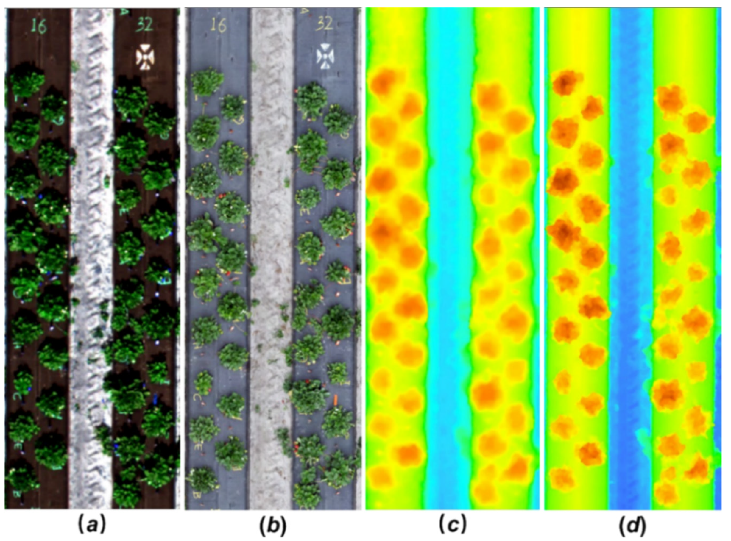
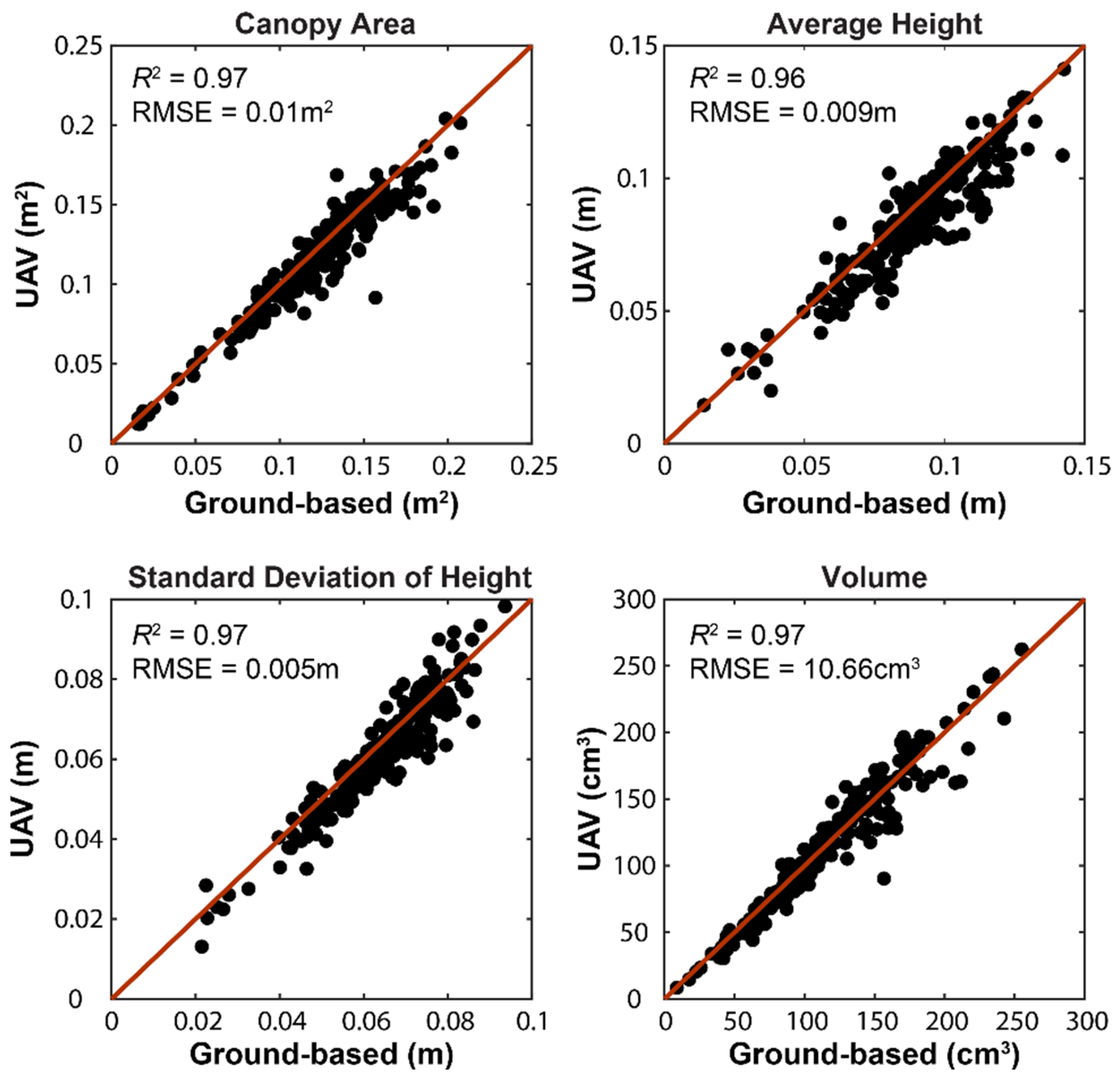
Figure 5 illustrates the orthomosaic imagery and DSM product generated from the ground-based and UAV images. Four strawberry canopy geometric parameters were calculated from both ground-based and UAV DSM products, including the canopy area, average height, standard deviation of canopy height and volume. The correlation between the ground-based and UAV image-derived canopy metrics is shown in Figure 6. Compared with the UAV image (1 cm), the ground-based DSM product with higher spatial resolution (2 mm) reveals more detail on the height gradient and texture of the strawberry canopy. However, there is little difference in the canopy metrics computed from these two types of DSM products. The R2 achieved 0.97, 0.96, 0.97 and 0.97 for the canopy area, average height, standard deviation of canopy height and volume, respectively. The result indicates that a resolution of 1 cm is sufficient to obtain geometric information on individual strawberry canopies.

Figure 5.
Comparison of ground-based imagery and UAV multispectral imagery: (a) UAV orthomosaic image with a spatial resolution of 1 cm; (b) ground-based orthomosaic image (1 mm); (c) UAV DSM product (1 cm); (d) ground-based DSM product (2 mm).
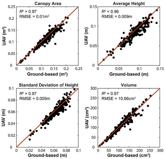
Figure 6.
Scatterplots showing ground-based and UAV image-derived strawberry canopy structural parameters, including the canopy area, average height, standard deviation of height and volume.
3.2. Modeling and Validation of Biomass
3.2.1. Variable Importance Evaluation
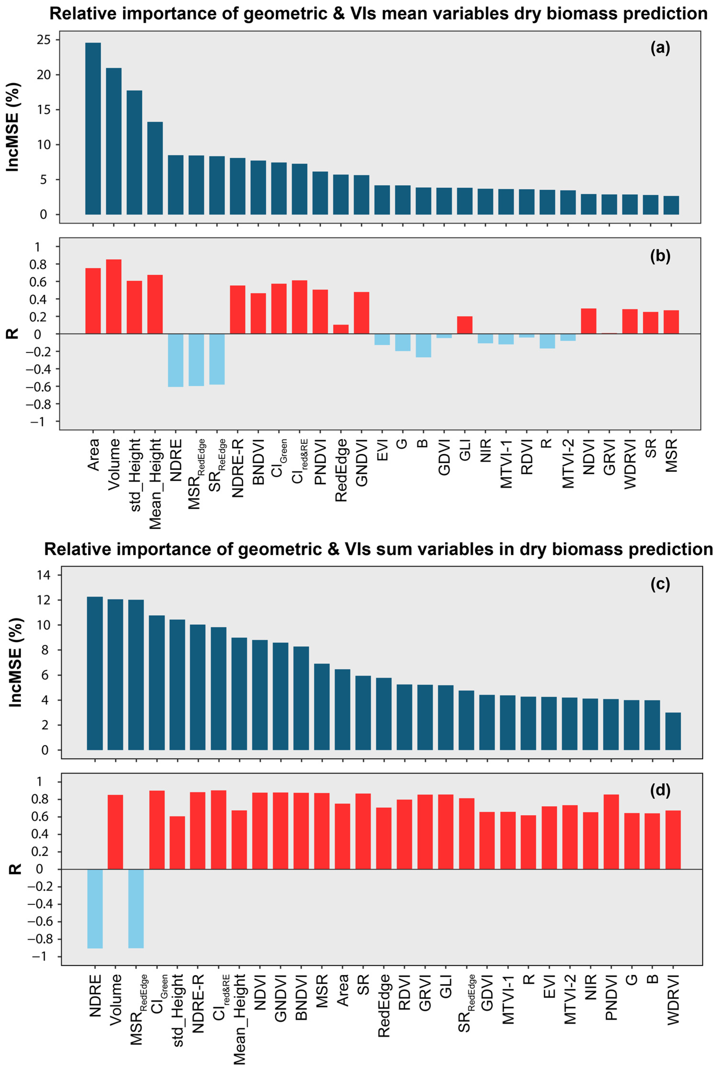
The image-based features in this study were of two types: (1) plant geometric properties, quantified as four structural traits—canopy area, volume, average height, and standard deviation of height; (2) two sets of spectral variables, including the original 5 band reflectance values and 20 vegetation indices (VIs), which potentially reflect the morphological (such as leaf density) and biochemical (e.g., water content, pigments) characteristics of strawberry plants [65]. When extracting the spectral information of strawberry plants, the mean and sum values of the VIs and spectral bands for all pixels within an individual plant canopy were calculated and used. We firstly used the Boruta R package to evaluate the relative importance of each feature to biomass estimation. All twenty-nine variables were confirmed to have an impact on the biomass modeling. The relative importance of each feature was assessed using the mean decrease accuracy (%IncMSE), which refers to the average increase in squared residuals after permuting the corresponding variable. A higher %IncMSE value indicates higher variable importance.
As shown in Figure 7a,b, the geometric features showed the most predictive power for predicting dry biomass. Among all VIs, the mean MSRRedEdge, SRRedEdge, NDRE and CIred&RE were most influential in the biomass estimation. Strikingly, the sum values of all pixels within each plant of the three VIs (MSRRedEdge, NDRE and CIred&RE) were the top ranked features for dry biomass prediction, even more important than the canopy area and volume, as shown in Figure 7c,d. The reason for this difference may be due to the fact that the VIs’ sum (VI mean × area) contains both structural and spectral information. To further observe the relationship between biomass and image-derived features, the distribution characteristics of six variables (the three geometric traits and the three VIs above) in different biomass intervals were computed and are shown in Figure 8. As expected, canopy area, average height and volume of height increased with the increase in the biomass. The mean SRRedEdge, MSRRedEdge and NDRE decreased with the increase in biomass.
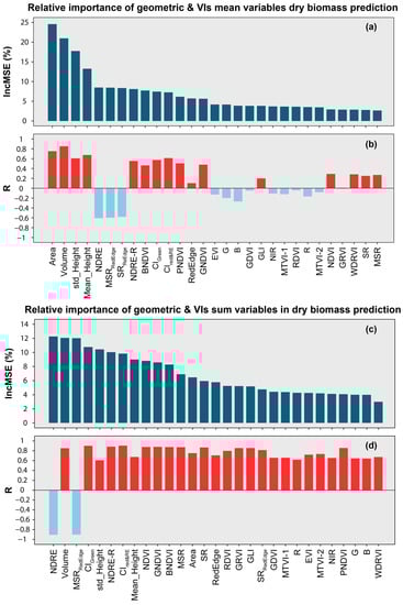
Figure 7.
The relative importance of image-based features in the prediction of strawberry biomass: (a) importance of geometric parameters and VI mean variables for modeling dry biomass; (b) correlation coefficients of geometric parameters and VI mean variables with dry biomass; (c) importance of geometric parameters and VI sum variables for modeling dry biomass; (d) correlation coefficients of geometric parameters and VI sum variables with dry biomass. The dark green strip represents the mean decrease accuracy (%IncMSE) of various variables. The red and cyan strips represent the positive and negative correlations between the study variable with the dry biomass, respectively.
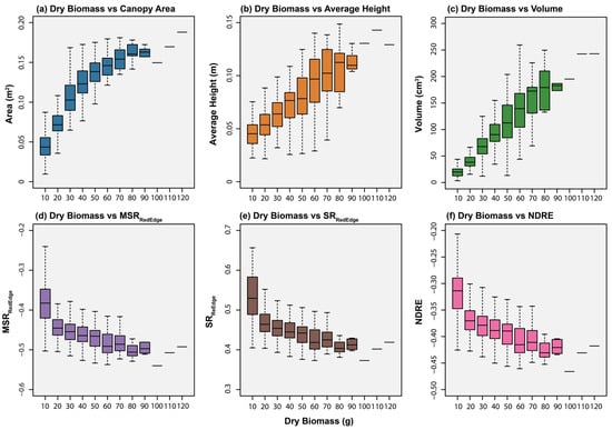
Figure 8.
Box plots showing the variations in strawberry canopy geometric parameters and VIs with the increase in dry biomass. (a): dry biomass vs. canopy area, (b): dry biomass vs. average height, (c): dry biomass vs. volume, (d): dry biomass vs. MSRRedEdge, (e): dry biomass vs. SRRedEdge, (f): dry biomass vs. NDRE. The x axis represents different biomass intervals. For dry biomass, the interval is set as 10. For example, “10” and “20” represent the ranges of [0, 10] and [10, 20], respectively.
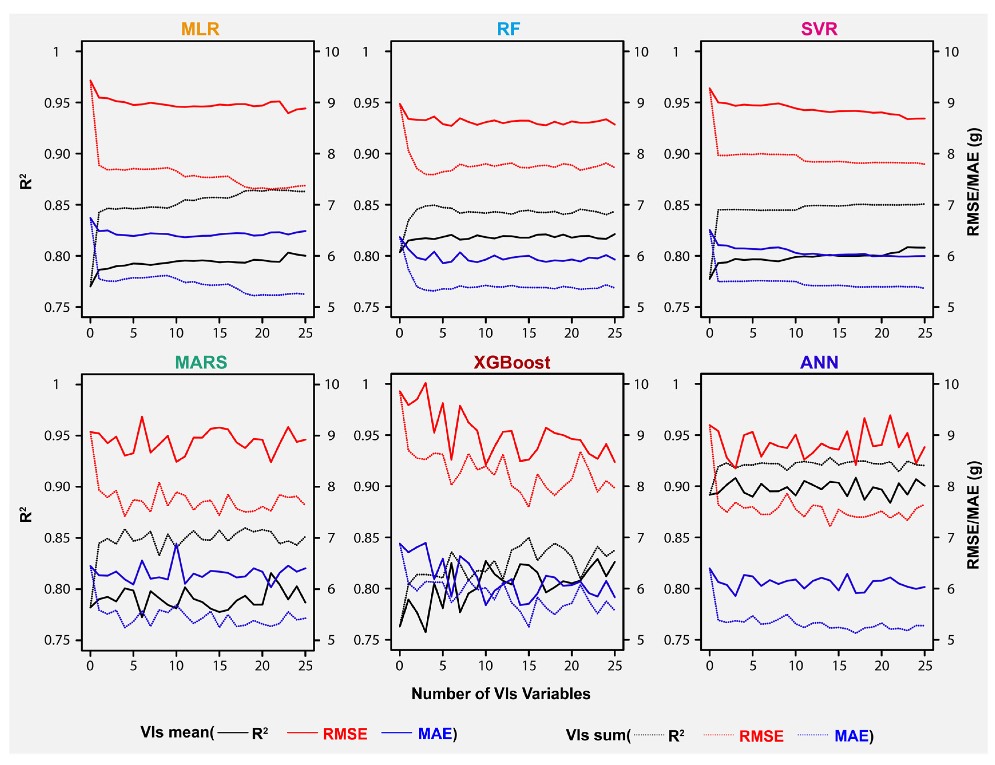
Next, we examined the model performance of the six regression methods, MLR, RF, SVR, MARS, XGBoost and ANN, by incorporating different numbers of VIs into the modeling (Figure 9). The validation accuracy of MLR, RF and SVR showed stabilized performance values after incorporating only a few VIs. The performance of MARS, XGBoost and ANN became fluctuant after VIs with low relative importance were imported into the model. Overall, the continued increase in the number of input VIs did not appear to remarkably improve the model performance. To avoid the overfitting and model instability caused by a large number of variables, we chose six VI parameters (MSRRedEdge, SRRedEdge, BNDVI, NDRE-R, NDRE and CIgreen) according to the relative importance and combined four geometric variables to evaluate the performance of the six regression models.
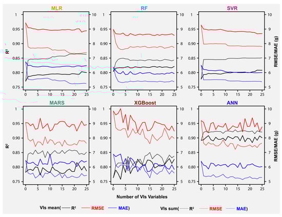
Figure 9.
Validation accuracy of six regression techniques using different numbers of input VIs. The number “0” indicates that only geometric parameters were used for the biomass prediction.
3.2.2. Performance of Prediction Methods in Strawberry Dry Biomass Prediction
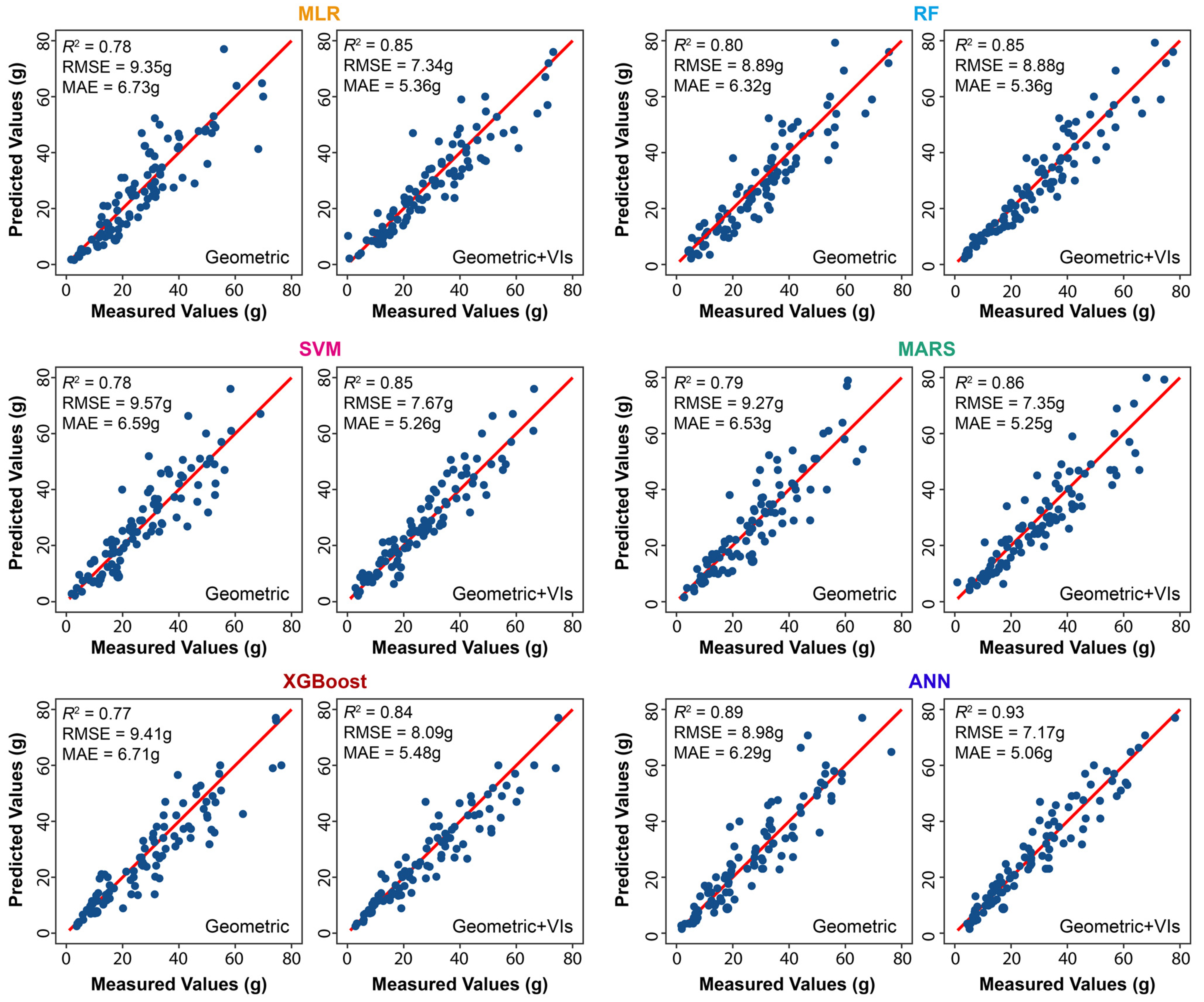
Table 4 shows the average five-fold CV results of six regression methods for strawberry dry biomass prediction. To assess the impact of VIs on biomass modeling, two types of feature combinations were used: (1) only geometric parameters (canopy area, average height, standard deviation of canopy height and volume); (2) geometric parameters and the six VIs input. Two methods of VI calculation (mean and sum) were also compared. The model performance was ranked as follows: (1) ANN > RF > MARS > SVM > MLR > XGBoost when only geometric variables were imported; (2) ANN > XGBoost > RF > MARS > SVM > MLR with both geometric variables and VI means as input; (3) ANN > <MARS > SVM > MLR > RF > XGBoost when both geometric variables and VI sums were used. The above ranking results are based on the R2 metric. Overall, the results indicate that the ANN significantly outperformed other models, with R2 of 0.89~0.93, RMSE of 7.16~8.98 g and MAE of 5.06~6.29 g. The RF seems more stable with different types of input variables than the other four machine learning methods. Compared with the VI mean calculation method, the use of the VI sum is more effective in improving the performance of the model. Figure 10 provides examples of the predicted dry biomass values compared to the field-based measurements using geometric variables and six VI sums as input.
Table 4.
Average five-fold CV results for the dry biomass models.
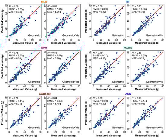
Figure 10.
Scatterplots of in-situ measured plant dry biomass vs. predicted values using six prediction models: MLR, RF, SVR, MARS, XGBoost and ANN. For each method, the performance was compared using only geometric parameters and all features (geometric parameters and VI sum variables).
4. Discussion
Our study used widely available technologies represented by the MicaSense multispectral camera mounted on a small UAV to predict strawberry canopy dry biomass weight. The five different bands of the MicaSense images were used to extract 4 geometric parameters and 20 vegetation indices. We firstly assessed the quality of the UAV DSM (1 cm spatial resolution) against higher-resolution (2 mm) DSM derived from ground-based imagery. The canopy geometric variables derived from the two datasets exhibited a high degree of consistency, with R2 above 0.96, which suggested that the one-centimeter UAV dataset is sufficient for strawberry biomass estimation.
Previous studies have demonstrated that spectral variables are the most used and effective remote sensing indicators for estimating plant biophysical properties (e.g., canopy nitrogen content, biomass and yield) [66,67,68]. The red-edge spectral region, located in the red-NIR transition zone, where the position of reflectivity changes drastically, was often referred to as a good indicator of leaf chlorophyll content [69]. Meanwhile, the red-edge band can alleviate the saturation problem of high biomass values to a certain extent [37,38]. In our study, the relative importance of four geometric parameters (area, volume, stand deviation of height and average height) and twenty-five spectral variables (5 spectral bands and 20 VIs) to the biomass modeling was evaluated and ranked. As expected, the geometric parameters reflecting the structural characteristics of the strawberry canopy were the top four variables. The R2 between dry biomass and canopy volume reached 0.703. As for the mean VIs of all pixels within each strawberry plant canopy, the MSRRedEdge, NDRE and CIred&RE appeared to be most influential on the biomass predictive model performance, with R2 in the range of [0.5, 0.6] between the three VIs and dry biomass. These results highlight the red-edge-related VIs as good biomass predictors. This is probably because these VIs may be sensitive to the canopy gap fraction and senescence change, and thus can effectively reflect the differences in canopy density or leaf weight properties among strawberry plants [70].
Unlike grasses and grain crops such as wheat, strawberries are dicots and have a more complex plant structure. Thus, two types of VI calculations (mean and sum) were performed for each plant, as described in Section 2.4.3. There was a certain degree of multi-collinearity between the 25 VIs (Figure S1 in the supplementary file). Machine learning techniques have been proven to effectively tackle the multi-collinearity problem and make full use of strongly collinear VIs in previous studies [71,72,73]. In this study, six regression techniques (MLR, RF, SVR, XGBoost, MARS and ANN) were adopted and examined for the biomass prediction. However, the increase in the number of VIs input did not result in a sustained improvement in model performance. The validation accuracy of MARS, XGBoost and ANN fluctuated after importing VIs of relatively low importance into the model, which may have been caused by overfitting. Therefore, we selected six VI variables combined with four geometric parameters to evaluate the above models.
The results show that ANN outperformed other models, with R2 of 0.89~0.93, RMSE of 7.16~8.98 g and MAE of 5.06~6.29 g. The performance of the other five models did not exhibit significant differences. For the VI calculation method, the sum of VI improved the model performance over the mean VI values. This result may be due to the nonlinear relationship between VIs and biomass unexplained by the VI mean. The addition of VIs increased the R2 from 0.77~0.80 to 0.83~0.86, and reduced the RMSE from 8.89~9.58 to 7.35~8.09 g and the MAE from 6.30~6.70 to 5.25~5.47 g, respectively. Overall, the combination of canopy structure and spectral information led to a noticeable increase in accuracy compared to using only geometric parameters.
5. Conclusions
In this study, six different regression methods were adopted to predict strawberry canopy dry biomass using UAV MicaSense multispectral images. These models were established using the canopy structural indicators extracted from DEM imagery and various vegetation indices (VIs) derived from the reflectance values of the five MicaSense bands. The results indicated the red-edge-related VIs (such as MSRRedEdge, NDRE, SRRedEdge and CIred&RE) to be most influential on model performance, apart from the structural parameters. The ANN model gave greater predictive ability than the other machine learning methods. This experiment demonstrated the potential application of UAV-captured canopy structural indicators, VIs and machine learning to estimate strawberry canopy biomass.
Supplementary Materials
The following supporting information can be downloaded at: https://www.mdpi.com/article/10.3390/rs14184511/s1, Figure S1: Correlation coefficient (R) among 29 variables, and Tables S1–S6: The optimal model hyperparameters for five machine learning models.
Author Contributions
Conceptualization, A.A.-E., V.W. and C.Z.; Methodology, C.Z. and A.A.-E.; Data curation, C.Z. and C.D.; Formal analysis, C.Z.; Project administration, A.A.-E. and V.W.; Software, C.D.; Supervision, A.A.-E. and V.W.; Validation, C.Z. and C.D.; Visualization, C.Z.; Writing—original draft preparation, C.Z.; Writing—review and editing, A.A.-E. and V.W. All authors have read and agreed to the published version of the manuscript.
Funding
This research received no external funding.
Data Availability Statement
The data that support the experiments of this study are available from the Gulf Coast Research and Education Center (GCREC) of the University of Florida. Restrictions apply to the availability of these data. Data (UAV imagery and ground-truth biomass measurements) are available from the corresponding author with the permission of GCREC.
Acknowledgments
The authors would like to acknowledge the Gulf Coast Research and Education field technical support staff and strawberry breeding program staff for their efforts in developing the data acquisition platform and field trials.
Conflicts of Interest
The authors declare no conflict of interest.
References
- Hofius, D.; Börnke, F.A. Photosynthesis, carbohydrate metabolism and source–sink relations. In Potato Biology and Biotechnology; Elsevier: Amsterdam, The Netherlands, 2007; pp. 257–285. [Google Scholar]
- Yoo, C.G.; Pu, Y.; Ragauskas, A.J. Measuring Biomass-Derived Products in Biological Conversion and Metabolic Process. In Metabolic Pathway Engineering; Springer: Berlin/Heidelberg, Germany, 2020; pp. 113–124. [Google Scholar]
- Johansen, K.; Morton, M.; Malbeteau, Y.; Aragon Solorio, B.J.L.; Almashharawi, S.; Ziliani, M.; Angel, Y.; Fiene, G.; Negrão, S.; Mousa, M. Predicting biomass and yield at harvest of salt-stressed tomato plants using UAV imagery. Int. Arch. Photogramm. Remote Sens. Spatial Inf. Sci. 2019, XLII-2/W13, 407–411. [Google Scholar] [CrossRef]
- Bendig, J.; Yu, K.; Aasen, H.; Bolten, A.; Bennertz, S.; Broscheit, J.; Gnyp, M.L.; Bareth, G. Combining UAV-based plant height from crop surface models, visible, and near infrared vegetation indices for biomass monitoring in barley. Int. J. Appl. Earth Obs. Geoinf. 2015, 39, 79–87. [Google Scholar] [CrossRef]
- Hensgen, F.; Bühle, L.; Wachendorf, M. The effect of harvest, mulching and low-dose fertilization of liquid digestate on above ground biomass yield and diversity of lower mountain semi-natural grasslands. Agric. Ecosyst. Environ. 2016, 216, 283–292. [Google Scholar] [CrossRef]
- Yuan, M.; Burjel, J.; Isermann, J.; Goeser, N.; Pittelkow, C. Unmanned aerial vehicle–based assessment of cover crop biomass and nitrogen uptake variability. J. Soil Water Conserv. 2019, 74, 350–359. [Google Scholar] [CrossRef]
- Zheng, C.; Abd-Elrahman, A.; Whitaker, V. Remote sensing and machine learning in crop phenotyping and management, with an emphasis on applications in strawberry farming. Remote Sens. 2021, 13, 531. [Google Scholar] [CrossRef]
- Yang, K.-W.; Chapman, S.; Carpenter, N.; Hammer, G.; McLean, G.; Zheng, B.; Chen, Y.; Delp, E.; Masjedi, A.; Crawford, M. Integrating crop growth models with remote sensing for predicting biomass yield of sorghum. in silico Plants 2021, 3, diab001. [Google Scholar] [CrossRef]
- Catchpole, W.; Wheeler, C. Estimating plant biomass: A review of techniques. Aust. J. Ecol. 1992, 17, 121–131. [Google Scholar] [CrossRef]
- Wang, T.; Liu, Y.; Wang, M.; Fan, Q.; Tian, H.; Qiao, X.; Li, Y. Applications of UAS in crop biomass monitoring: A review. Front. Plant Sci. 2021, 12, 616689. [Google Scholar] [CrossRef]
- Chen, D.; Shi, R.; Pape, J.-M.; Neumann, K.; Arend, D.; Graner, A.; Chen, M.; Klukas, C. Predicting plant biomass accumulation from image-derived parameters. GigaScience 2018, 7, giy001. [Google Scholar] [CrossRef]
- Yang, S.; Feng, Q.; Liang, T.; Liu, B.; Zhang, W.; Xie, H. Modeling grassland above-ground biomass based on artificial neural network and remote sensing in the Three-River Headwaters Region. Remote Sens. Environ. 2018, 204, 448–455. [Google Scholar] [CrossRef]
- Chao, Z.; Liu, N.; Zhang, P.; Ying, T.; Song, K. Estimation methods developing with remote sensing information for energy crop biomass: A comparative review. Biomass Bioenergy 2019, 122, 414–425. [Google Scholar] [CrossRef]
- Réjou-Méchain, M.; Barbier, N.; Couteron, P.; Ploton, P.; Vincent, G.; Herold, M.; Mermoz, S.; Saatchi, S.; Chave, J.; De Boissieu, F. Upscaling forest biomass from field to satellite measurements: Sources of errors and ways to reduce them. Surv. Geophys. 2019, 40, 881–911. [Google Scholar] [CrossRef]
- Rodríguez-Veiga, P.; Quegan, S.; Carreiras, J.; Persson, H.J.; Fransson, J.E.; Hoscilo, A.; Ziółkowski, D.; Stereńczak, K.; Lohberger, S.; Stängel, M. Forest biomass retrieval approaches from earth observation in different biomes. Int. J. Appl. Earth Obs. Geoinf. 2019, 77, 53–68. [Google Scholar] [CrossRef]
- Santoro, M.; Cartus, O.; Carvalhais, N.; Rozendaal, D.; Avitabile, V.; Araza, A.; De Bruin, S.; Herold, M.; Quegan, S.; Rodríguez-Veiga, P. The global forest above-ground biomass pool for 2010 estimated from high-resolution satellite observations. Earth Syst. Sci. Data 2021, 13, 3927–3950. [Google Scholar] [CrossRef]
- Ahmad, A.; Gilani, H.; Ahmad, S.R. Forest aboveground biomass estimation and mapping through high-resolution optical satellite imagery—A literature review. Forests 2021, 12, 914. [Google Scholar] [CrossRef]
- Naik, P.; Dalponte, M.; Bruzzone, L. Prediction of Forest Aboveground Biomass Using Multitemporal Multispectral Remote Sensing Data. Remote Sens. 2021, 13, 1282. [Google Scholar] [CrossRef]
- Zheng, H.; Cheng, T.; Zhou, M.; Li, D.; Yao, X.; Tian, Y.; Cao, W.; Zhu, Y. Improved estimation of rice aboveground biomass combining textural and spectral analysis of UAV imagery. Precis. Agric. 2019, 20, 611–629. [Google Scholar] [CrossRef]
- Yue, J.; Yang, G.; Tian, Q.; Feng, H.; Xu, K.; Zhou, C. Estimate of winter-wheat above-ground biomass based on UAV ultrahigh-ground-resolution image textures and vegetation indices. ISPRS J. Photogramm. Remote Sens. 2019, 150, 226–244. [Google Scholar] [CrossRef]
- Toda, Y.; Kaga, A.; Kajiya-Kanegae, H.; Hattori, T.; Yamaoka, S.; Okamoto, M.; Iwata, H. Genomic prediction modeling of soybean biomass using UAV-based remote sensing and longitudinal model parameters. Plant Genome 2021, 14, e20157. [Google Scholar] [CrossRef]
- Geng, L.; Che, T.; Ma, M.; Tan, J.; Wang, H. Corn biomass estimation by integrating remote sensing and long-term observation data based on machine learning techniques. Remote Sens. 2021, 13, 2352. [Google Scholar] [CrossRef]
- Dong, T.; Liu, J.; Qian, B.; He, L.; Liu, J.; Wang, R.; Jing, Q.; Champagne, C.; McNairn, H.; Powers, J. Estimating crop biomass using leaf area index derived from Landsat 8 and Sentinel-2 data. ISPRS J. Photogramm. Remote Sens. 2020, 168, 236–250. [Google Scholar] [CrossRef]
- Stagakis, S.; Markos, N.; Sykioti, O.; Kyparissis, A. Monitoring canopy biophysical and biochemical parameters in ecosystem scale using satellite hyperspectral imagery: An application on a Phlomis fruticosa Mediterranean ecosystem using multiangular CHRIS/PROBA observations. Remote Sens. Environ. 2010, 114, 977–994. [Google Scholar] [CrossRef]
- Yang, G.; Liu, J.; Zhao, C.; Li, Z.; Huang, Y.; Yu, H.; Xu, B.; Yang, X.; Zhu, D.; Zhang, X. Unmanned aerial vehicle remote sensing for field-based crop phenotyping: Current status and perspectives. Front. Plant Sci. 2017, 8, 1111. [Google Scholar] [CrossRef] [PubMed]
- Tsouros, D.C.; Bibi, S.; Sarigiannidis, P.G. A review on UAV-based applications for precision agriculture. Information 2019, 10, 349. [Google Scholar] [CrossRef]
- Xie, C.; Yang, C. A review on plant high-throughput phenotyping traits using UAV-based sensors. Comput. Electron. Agric. 2020, 178, 105731. [Google Scholar] [CrossRef]
- Shi, Y.; Thomasson, J.A.; Murray, S.C.; Pugh, N.A.; Rooney, W.L.; Shafian, S.; Rajan, N.; Rouze, G.; Morgan, C.L.; Neely, H.L. Unmanned aerial vehicles for high-throughput phenotyping and agronomic research. PLoS ONE 2016, 11, e0159781. [Google Scholar] [CrossRef]
- Toth, C.; Jóźków, G. Remote sensing platforms and sensors: A survey. ISPRS J. Photogramm. Remote Sens. 2016, 115, 22–36. [Google Scholar] [CrossRef]
- Westoby, M.J.; Brasington, J.; Glasser, N.F.; Hambrey, M.J.; Reynolds, J.M. ‘Structure-from-Motion’photogrammetry: A low-cost, effective tool for geoscience applications. Geomorphology 2012, 179, 300–314. [Google Scholar] [CrossRef]
- De Souza, C.H.W.; Lamparelli, R.A.C.; Rocha, J.V.; Magalhães, P.S.G. Height estimation of sugarcane using an unmanned aerial system (UAS) based on structure from motion (SfM) point clouds. Int. J. Remote Sens. 2017, 38, 2218–2230. [Google Scholar] [CrossRef]
- Fraser, B.T.; Congalton, R.G. Issues in Unmanned Aerial Systems (UAS) data collection of complex forest environments. Remote Sens. 2018, 10, 908. [Google Scholar] [CrossRef] [Green Version]
- Fu, Y.; Yang, G.; Song, X.; Li, Z.; Xu, X.; Feng, H.; Zhao, C. Improved estimation of winter wheat aboveground biomass using multiscale textures extracted from UAV-based digital images and hyperspectral feature analysis. Remote Sens. 2021, 13, 581. [Google Scholar] [CrossRef]
- Johansen, K.; Morton, M.J.; Malbeteau, Y.; Aragon, B.; Al-Mashharawi, S.; Ziliani, M.G.; Angel, Y.; Fiene, G.; Negrão, S.; Mousa, M.A. Predicting biomass and yield in a tomato phenotyping experiment using UAV imagery and random forest. Front. Artif. Intell. 2020, 3, 28. [Google Scholar] [CrossRef] [PubMed]
- Wang, F.; Yang, M.; Ma, L.; Zhang, T.; Qin, W.; Li, W.; Zhang, Y.; Sun, Z.; Wang, Z.; Li, F. Estimation of Above-Ground Biomass of Winter Wheat Based on Consumer-Grade Multi-Spectral UAV. Remote Sens. 2022, 14, 1251. [Google Scholar] [CrossRef]
- Che, S.; Du, G.; Wang, N.; He, K.; Mo, Z.; Sun, B.; Chen, Y.; Cao, Y.; Wang, J.; Mao, Y. Biomass estimation of cultivated red algae Pyropia using unmanned aerial platform based multispectral imaging. Plant Methods 2021, 17, 1–13. [Google Scholar] [CrossRef] [PubMed]
- Mutanga, O.; Skidmore, A.K. Narrow band vegetation indices overcome the saturation problem in biomass estimation. Int. J. Remote Sens. 2004, 25, 3999–4014. [Google Scholar] [CrossRef]
- Tesfaye, A.A.; Awoke, B.G. Evaluation of the saturation property of vegetation indices derived from sentinel-2 in mixed crop-forest ecosystem. Spat. Inf. Res 2021, 29, 109–121. [Google Scholar] [CrossRef]
- Guan, Z.; Abd-Elrahman, A.; Fan, Z.; Whitaker, V.M.; Wilkinson, B. Modeling strawberry biomass and leaf area using object-based analysis of high-resolution images. ISPRS J. Photogramm. Remote Sens. 2020, 163, 171–186. [Google Scholar] [CrossRef]
- Abd-Elrahman, A.; Guan, Z.; Dalid, C.; Whitaker, V.; Britt, K.; Wilkinson, B.; Gonzalez, A. Automated canopy delineation and size metrics extraction for strawberry dry weight modeling using raster analysis of high-resolution imagery. Remote Sens. 2020, 12, 3632. [Google Scholar] [CrossRef]
- Abd-Elrahman, A.; Pande-Chhetri, R.; Vallad, G. Design and development of a multi-purpose low-cost hyperspectral imaging system. Remote Sens. 2011, 3, 570–586. [Google Scholar] [CrossRef]
- Abd-Elrahman, A.; Sassi, N.; Wilkinson, B.; Dewitt, B. Georeferencing of mobile ground-based hyperspectral digital single-lens reflex imagery. J. Appl. Remote Sens. 2016, 10, 014002. [Google Scholar] [CrossRef] [Green Version]
- Carlson, T.N.; Ripley, D.A. On the relation between NDVI, fractional vegetation cover, and leaf area index. Remote Sens. Environ. 1997, 62, 241–252. [Google Scholar] [CrossRef]
- Roujean, J.-L.; Breon, F.-M. Estimating PAR absorbed by vegetation from bidirectional reflectance measurements. Remote Sens. Environ. 1995, 51, 375–384. [Google Scholar] [CrossRef]
- Banerjee, B.P.; Sharma, V.; Spangenberg, G.; Kant, S. Machine learning regression analysis for estimation of crop emergence using multispectral UAV imagery. Remote Sens. 2021, 13, 2918. [Google Scholar] [CrossRef]
- Gitelson, A.A.; Merzlyak, M.N. Remote sensing of chlorophyll concentration in higher plant leaves. Adv. Space Res. 1998, 22, 689–692. [Google Scholar] [CrossRef]
- Strong, C.J.; Burnside, N.G.; Llewellyn, D. The potential of small-Unmanned Aircraft Systems for the rapid detection of threatened unimproved grassland communities using an Enhanced Normalized Difference Vegetation Index. PLoS ONE 2017, 12, e0186193. [Google Scholar] [CrossRef]
- Motohka, T.; Nasahara, K.N.; Oguma, H.; Tsuchida, S. Applicability of green-red vegetation index for remote sensing of vegetation phenology. Remote Sens. 2010, 2, 2369–2387. [Google Scholar] [CrossRef]
- Liu, X.; Wang, L. Feasibility of using consumer-grade unmanned aerial vehicles to estimate leaf area index in mangrove forest. Remote Sens. Lett. 2018, 9, 1040–1049. [Google Scholar] [CrossRef]
- Haboudane, D.; Miller, J.R.; Pattey, E.; Zarco-Tejada, P.J.; Strachan, I.B. Hyperspectral vegetation indices and novel algorithms for predicting green LAI of crop canopies: Modeling and validation in the context of precision agriculture. Remote Sens. Environ. 2004, 90, 337–352. [Google Scholar] [CrossRef]
- Wang, F.-M.; Huang, J.-F.; Tang, Y.-L.; Wang, X.-Z. New vegetation index and its application in estimating leaf area index of rice. Rice Sci. 2007, 14, 195–203. [Google Scholar] [CrossRef]
- Huete, A.; Didan, K.; Miura, T.; Rodriguez, E.P.; Gao, X.; Ferreira, L.G. Overview of the radiometric and biophysical performance of the MODIS vegetation indices. Remote Sens. Environ. 2002, 83, 195–213. [Google Scholar] [CrossRef]
- Gitelson, A.A. Wide dynamic range vegetation index for remote quantification of biophysical characteristics of vegetation. J. Plant Physiol. 2004, 161, 165–173. [Google Scholar] [CrossRef] [PubMed]
- Jordan, C.F. Derivation of leaf-area index from quality of light on the forest floor. Ecology 1969, 50, 663–666. [Google Scholar] [CrossRef]
- Santos, A.; Lacerda, L.; Gobbo, S.; Tofannin, A.; Silva, R.; Vellidis, G. Using remote sensing to map in-field variability of peanut maturity. Precis. Agric. 2019, 19, 91–101. [Google Scholar]
- Chen, J.M. Evaluation of vegetation indices and a modified simple ratio for boreal applications. Can. J. Remote Sens. 1996, 22, 229–242. [Google Scholar] [CrossRef]
- Gitelson, A.A.; Gritz, Y.; Merzlyak, M.N. Relationships between leaf chlorophyll content and spectral reflectance and algorithms for non-destructive chlorophyll assessment in higher plant leaves. J. Plant Physiol. 2003, 160, 271–282. [Google Scholar] [CrossRef]
- Thompson, C.N.; Guo, W.; Sharma, B.; Ritchie, G.L. Using normalized difference red edge index to assess maturity in cotton. Crop Sci. 2019, 59, 2167–2177. [Google Scholar] [CrossRef]
- Uyanık, G.K.; Güler, N. A study on multiple linear regression analysis. Procedia-Soc. Behav. Sci. 2013, 106, 234–240. [Google Scholar] [CrossRef]
- Boser, B.E.; Guyon, I.M.; Vapnik, V.N. A training algorithm for optimal margin classifiers. In Proceedings of the Fifth Annual Workshop on Computational Learning Theory, Pittsburgh, PA, USA, 27–29 July 1992; pp. 144–152. [Google Scholar]
- Drucker, H.; Burges, C.J.; Kaufman, L.; Smola, A.; Vapnik, V. Support vector regression machines. Adv. Neural Inf. Processing Syst. 1996, 9, 155–161. [Google Scholar]
- Friedman, J.H. Multivariate adaptive regression splines. Ann. Stat. 1991, 19, 1–67. [Google Scholar] [CrossRef]
- Chen, T.; Guestrin, C. Xgboost: A scalable tree boosting system. In Proceedings of the 22nd Acm Sigkdd International Conference on Knowledge Discovery and Data Mining, San Francisco, CA, USA, 13–17 August 2016; pp. 785–794. [Google Scholar]
- Yue, J.; Feng, H.; Yang, G.; Li, Z. A comparison of regression techniques for estimation of above-ground winter wheat biomass using near-surface spectroscopy. Remote Sens. 2018, 10, 66. [Google Scholar] [CrossRef]
- Xue, J.; Su, B. Significant remote sensing vegetation indices: A review of developments and applications. J. Sens. 2017, 2017, 1353691. [Google Scholar] [CrossRef]
- Lee, H.; Wang, J.; Leblon, B. Using linear regression, random forests, and support vector machine with unmanned aerial vehicle multispectral images to predict canopy nitrogen weight in corn. Remote Sens. 2020, 12, 2071. [Google Scholar] [CrossRef]
- Maimaitijiang, M.; Sagan, V.; Sidike, P.; Hartling, S.; Esposito, F.; Fritschi, F.B. Soybean yield prediction from UAV using multimodal data fusion and deep learning. Remote Sens. Environ. 2020, 237, 111599. [Google Scholar] [CrossRef]
- Santos, A.F.; Lacerda, L.N.; Rossi, C.; Moreno, L.d.A.; Oliveira, M.F.; Pilon, C.; Silva, R.P.; Vellidis, G. Using UAV and Multispectral Images to Estimate Peanut Maturity Variability on Irrigated and Rainfed Fields Applying Linear Models and Artificial Neural Networks. Remote Sens. 2021, 14, 93. [Google Scholar] [CrossRef]
- Wu, C.; Niu, Z.; Tang, Q.; Huang, W. Estimating chlorophyll content from hyperspectral vegetation indices: Modeling and validation. Agric. For. Meteorol. 2008, 148, 1230–1241. [Google Scholar] [CrossRef]
- Xie, Q.; Dash, J.; Huang, W.; Peng, D.; Qin, Q.; Mortimer, H.; Casa, R.; Pignatti, S.; Laneve, G.; Pascucci, S. Vegetation indices combining the red and red-edge spectral information for leaf area index retrieval. IEEE J. Sel. Top. Appl. Earth Obs. Remote Sens. 2018, 11, 1482–1493. [Google Scholar] [CrossRef]
- Yue, J.; Yang, G.; Feng, H. Comparative of remote sensing estimation models of winter wheat biomass based on random forest algorithm. Trans. Chin. Soc. Agric. Eng. 2016, 32, 175–182. [Google Scholar]
- Yuan, H.; Yang, G.; Li, C.; Wang, Y.; Liu, J.; Yu, H.; Feng, H.; Xu, B.; Zhao, X.; Yang, X. Retrieving soybean leaf area index from unmanned aerial vehicle hyperspectral remote sensing: Analysis of RF, ANN, and SVM regression models. Remote Sens. 2017, 9, 309. [Google Scholar] [CrossRef]
- Guan, Z.; Abd-Elrahman, A.; Whitaker, V.; Agehara, S.; Wilkinson, B.; Gastellu-Etchegorry, J.P.; Dewitt, B. Radiative transfer image simulation using L-system modeled strawberry canopies. Remote Sens. 2022, 14, 548. [Google Scholar] [CrossRef]


Publisher’s Note: MDPI stays neutral with regard to jurisdictional claims in published maps and institutional affiliations. |
© 2022 by the authors. Licensee MDPI, Basel, Switzerland. This article is an open access article distributed under the terms and conditions of the Creative Commons Attribution (CC BY) license (https://creativecommons.org/licenses/by/4.0/).