Abstract
The atmospheric boundary layer height () is a key parameter in the vertical transport of mass, energy, moisture, and chemical species between the surface and the free atmosphere. There is a lack of long-term and continuous observations of , however, particularly for remote regions, such as the Amazon forest. Reanalysis products, such as ERA5, can fill this gap by providing temporally and spatially resolved information on . In this work, we evaluate the ERA5 estimates of (-ERA5) for two locations in the Amazon and corrected them by means of ceilometer, radiosondes, and SODAR measurements (-experimental). The experimental data were obtained at the remote Amazon Tall Tower Observatory (ATTO) with its pristine tropical forest cover and the T3 site downwind of the city of Manaus with a mixture of forest (), pasture (), and rivers (). We focus on the rather typical year 2014 and the El Niño year 2015. The comparison of the experimental vs. ERA5 data yielded the following results: (i) -ERA5 underestimates -experimental daytime at the T3 site for both years 2014 (30%, underestimate) and 2015 (15%, underestimate); (ii) -ERA5 overestimates -experimental daytime at ATTO site (12%, overestimate); (iii) during nighttime, no significant correlation between the -experimental and -ERA5 was observed. Based on these findings, we propose a correction for the daytime -ERA5, for both sites and for both years, which yields a better agreement between experimental and ERA5 data. These results and corrections are relevant for studies at ATTO and the T3 site and can likely also be applied at further locations in the Amazon.
1. Introduction
The planetary boundary layer (PBL) is the lowest portion of the troposphere and is directly and dynamically influenced by the Earth’s surface [1,2]. These surface–atmosphere interactions occur on short timescales and play a crucial role in the development of the PBL height (). The PBL is also influenced by atmospheric conditions, topographic characteristics, and the type of land cover. Thus, is an important parameter for many meteorological applications, such as air quality monitoring, cloud formation and evolution, land and ocean surface fluxes, and the atmospheric hydrological cycle [3]. As the PBL height represents the depth of the vertical turbulent mixing and, therefore, defines the enrichment or dilution of pollutants close to the surface, it is an essential parameter in air quality monitoring and simulations [4]. The PBL height is, further, a key factor in numerical weather forecasts, since the base height of the clouds is usually located closely to . Furthermore, the PBL evolution from its nocturnal state to convective mixing determines the cloud development and transition from shallow to deep convection [5].
The values can be obtained from radiosonde launches [6] as well as from various remote sensing tools, such as ground-based LIDAR [7,8,9], SODAR [10], ceilometer [11,12], and aircraft sounding [13]. These methods typically provide high-resolution profiles of the lower troposphere, however, are typically restricted to local measurements and limited measurement periods. Logistical and budgetary constraints further strongly limit continuous measurements in remote areas, which entails that experimental retrievals are sparse over oceans, mountains, deserts, and large forests. A framework for satellite-based estimates is being developed [14,15], providing a good spatial coverage [14,16,17,18], however, with relatively low accuracy [19,20,21].
Reanalysis data are a promising alternative to obtain for different and especially remote areas of the world. The reanalysis system combines observational and modeling data by assimilating a variety of measurements, ranging from in situ to space-borne data, into weather prediction models. A main strength of reanalysis products is their spatiotemporal continuity, which enables long-term studies. A good example is the fifth generation of the European Centre for Medium-Range Weather Forecasts (ECMWF) atmospheric reanalysis (ERA5) [22], which is an upgrade of the previous ERA-Interim [23]. This dataset provides a good representation of the atmosphere and is being used worldwide – especially for values [24,25]—as it provides data where observational information is not available.
Intercomparisons between experimental data, such as radiosonde and LIDAR, on one hand, and ERA5 reanalysis data, on the other, were conducted in several previous studies. Zhang et al. [25] showed that the ERA5 values over the US exceed corresponding aircraft observations by 18–41%. This overestimation might be caused by different kinetic or thermodynamic assumptions used in the ERA5 estimates. Recently, [26] compared at a tropical site in western India using different estimates from satellite, radiosondes, and ERA5 outputs. They found that ERA5 underestimates the daytime ceilometer observations by 200–500 m. Unfortunately, they did not provide any information of corresponding comparison during nighttime. Madona et al. [27] compared the ERA5 outputs with radiosonde data for a long period (1978–2018) over Europe. They also analyzed the nighttime and daytime values for both atmospheric stability classes (unstable/daytime and stable/nighttime). They found that ERA5 is able to represent the observations at the Lindenberg Observatory in Germany reasonably well. Ref. [24] analyzed the climatology of ERA5-derived from 8 sites over the Korean peninsula and surrounding sea over a 10-year period. Their results show that ERA5 outputs agree reasonably well with radiosonde observations, although with significant diurnal and seasonal variability. They found an average correlation coefficient of around 0.7 for both timescales. The authors emphasize the importance of the soil moisture/surface sensible heat fluxes in modulating the PBL height. Remarkably, the authors also found a increasing trend in over the period of their study and associated this with potential effects of climate change. Ref. [28] established a daytime climatology based on different datasets (i.e., ERA5, MERRA-2, JRA-55, and NCEP-2). They analyzed around 300 stations (but none over Amazonia) during the period from 2012 up to 2019 and found that all reanalysis products underestimate the observations. In this study, the ERA5 provided the best results relative to radiosondes, however, with a negative bias (around −130 m). The study does not provide information on the nighttime period.
Over the Amazon region, several previous studies have investigated , mainly using radiosonde data collected during field campaigns [29,30,31,32,33,34]. Ref. [30] were among the first to show that values are greater above pasture than above forest regions. Ref. [33] recently evaluated the diurnal cycle of in two contrasting years, 2014 (typical year) and 2015 (El Niño year). For this, they used a wide suite of instruments (radiosonde, SODAR, ceilometer, wind profiler, LIDAR, and microwave radiometer) installed during the GoAmazon 2014/2015 campaign [35]. They found that the ceilometer is the best instrument to describe the PBL height once compared with in situ radiosonde measurements. Additionally, the El Niño year substantially influenced the growth phase of the daytime PBL, with a increase in its rate. In another approach, ref. [36] analyzed the PBL structure over two tropical forests in Central Amazonia, using observations and a numerical high-resolution model (large eddy simulation models—LES). The results, based on turbulent kinetic energy analysis, conclude that the boundary layer structure is strongly influenced by the presence of topography (hills and valleys) that can also trigger horizontal heterogeneity. Ref. [37] used observations and numerical model outputs for Amazonia to show that heat and moisture transports from the sub-cloud into the cloud layer are not well represented by regular reanalysis, such as ERA5.
This paper has the goal to better understand the PBL evolution by comparing multiple instruments and ERA5 simulations for two distinct years and for two distinct surface covers in Central Amazonia. The extensive observational data used here were collected during GoAmazon 2014/15 [35] and the ATTO project [38] as two major recent field experiments in Central Amazonia. The convective boundary layer (CBL) and the nocturnal boundary layer (NBL) were analyzed independently. We derived from ERA5 and propose a correction for this data based on the observational results. This comparatively simple correction is meant to allow the scientific community to use the ERA5 in a more reliable way and it represents a new parameterization for the retrieval in ERA5. To out knowledge, this is the first study proposing a correction to the values from ERA5 for the Amazon region.
2. Methods and Materials
2.1. Study Sites
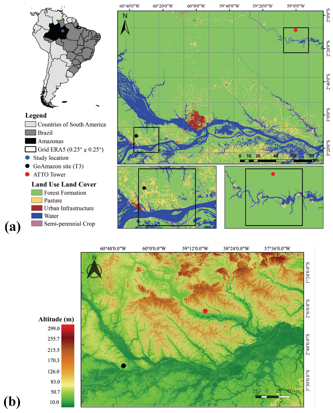
The study was carried out using data from two experimental sites located in Central Amazonia, as shown in Figure 1. The first one is called T3 site (, and 60 m of elevation above sea level) and was part of the Green Ocean Amazon Project (GoAmazon, http://campaign.arm.gov/Goamazon2014/, accessed on 25 July 2022) [35]. It is located in a pasture area north of the municipality of Manacapuru in the state of Amazonas. The second site is called Amazon Tall Tower Observatory (ATTO) and is installed in a region of pristine tropical forest (, and 130 m of elevation above sea level) about 150 km northeast of the city of Manaus, in the Uatumã Sustainable Development Reserve [38]. The T3 site is quite flat [35], a common feature for Amazonian regions located close to large rivers. On the other hand, the ATTO site has a slightly more accentuated orography, common to terra firme forests in the Amazon region [36,39].
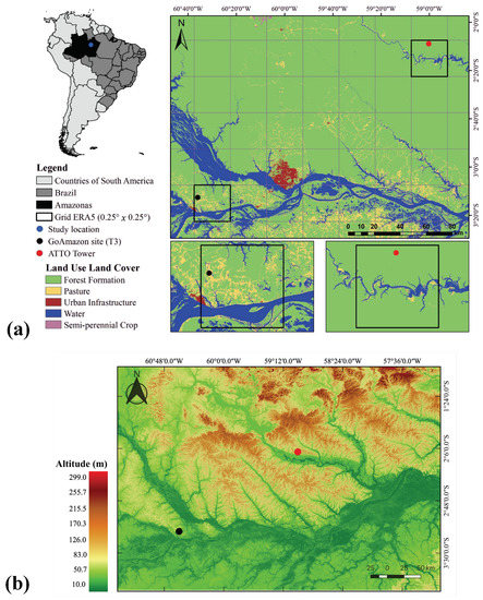
Figure 1.
(a) Geographic locations of the experimental sites T3 and ATTO in the Amazon basin. (b) Topography of the study region.
The climate in Amazonia is strongly associated with the rainfall distribution, with a wet (from February up to May) and a dry (from August to October) season. The temperature cycle is almost absent and its seasonal variation is around 2 °C. The energy partitioning between sensible and latent heat fluxes at the surface is strongly dependent on this rainfall distribution/soil moisture content [40].
For the current study, data from the GoAmazon project were used for the rainy quarters (named wet season) from February up to April, and for the the dry quarters (named dry season) from August up to October for two different years: 2014 can be considered a typical year in terms of rainfall distribution, whereas 2015 was largely affected by the strong El Niños at that time [33]. For ATTO, data from 31 October to 30 November 2015 were used, as both ceilometer and radiosonde data were available in this timeframe. For the GoAmazon analysis, the wet season (2014 and 2015) consisted of 89 days, which represents 2136 h of measurement, while the dry season (2014 and 2015) consisted of 92 days, representing 2208 h. For ATTO analysis, it was only 30 days (representing 720 h).
2.2. Radiosonde
At the T3 site, the values were derived from radiosondes (RS) using Vaisala sondes (RS92SVP) launched at standard synoptic times (GMT-4 h), at 02:00, 08:00, 11:00, 14:00, and 20:00 local time (LT). For the ATTO site, the radiosondes were made with the German system Graw DFM-09, launched at 02:00, 06:00, 08:00, 11:00, 14:00, 18:00, and 20:00 LT.
From the vertical profiles of the RS launches, the potential temperature () and specific humidity (q) were calculated, which then allowed to calculate the PBL height as follows: in its daytime phase (CBL), the heights were identified by the profile method [41,42], in which is the vertical level with an increase in and a reduction in q, for three or more layers (vertical bins). In the night phase (NBL), heights were determined where the vertical gradient was null or less than a defined number () from the surface [42,43].
2.3. Ceilometer
The values were also monitored in both experimental areas using two ceilometers. At the T3 site, a ceilometer model CL31 from Vaisala Inc. (Helsinki, Finland) was used, while at the ATTO site, a ceilometer model CHM15k (Jenoptik AG, Jena, Germany, now sold by Lufft (https://www.lufft.com/de-de/produkte/wolken-schneehoehensensoren-306/ceilometer-chm-15k-nimbus-2093/; accessed on 25 July 2022) was installed. Both instruments are LIDAR-type remote sensing techniques that record the intensity of the optical backscatter in the near-infrared wavelength (between 900 and 1100 nm) by emitting an autonomous vertical pulse. The LIDAR measurements rely on the aerosol concentration in the atmosphere. In the ABL, the aerosol concentration is high compared to the free atmosphere above, and this contrast is the basis for PBL height detection from LIDAR measurements [44]. These measurements are used to produce derived products that are recorded: the height of the cloud base, the retrieval of the particle backscatter coefficient, and PBL height [33,45,46].
The amount of backscattered light is detected in high temporal resolution for a maximum height of approximately 10 km and maximal sensitivity ∼100 m [46,47]. Thus, previous studies have shown that the ceilometer is a powerful tool to measure during its daily cycle (day and night phases) at a high level of detail [46,47,48]. The standard procedure for the PBL heights determination from Vaisala ceilometers is the software package BL-View developed by the manufacturer (for more details, see [49]).
The PBL heights variability, estimated from ceilometers, can vary from 100 m for wet conditions, for example, in the Amazonia [33], up to 200 m for dry conditions, for example, in deserts [50]. It should be noted that the T3 site is more polluted than ATTO, which entails that the measurements of the PBL top there are more robust. At very clean locations, such as the pristine forest at ATTO, the PBL height can sometimes be difficult to identify [11].
2.4. SODAR
For the T3 area, data from a SODAR (sound detection and ranging) (model SODAR MFAS and RASS A032002, Scintec, Rottenburg, Germany) were also used to measure the NBL height. This instrument provided wind speed and wind direction measurements every 30 min of the vertical profiles from the surface up to 400 m. The height of the NBL was determined using the maximum wind height (jet) methodology [33,43].
2.5. ERA5 Reanalysis Dataset
ERA5 is the fifth generation of atmospheric reanalysis of the global climate, produced by the assimilation of several observational datasets from satellites and radiosondes. It covers the entire global atmosphere and provides spatial and temporal data products [22]. The ERA5 data have 37 pressure levels with hourly time steps, and horizontal grid resolution of × , which represents a spatial size of around 30 km near the Equator. Therefore, we chose the grid where the experimental site is located (Figure 1). As the lower forcing for the model is dependent of the type of vegetation, a synthesis of its land use/land cover is shown in Table 1.

Table 1.
Land use and land cover (LULC) within the ERA5 grid for the two experimental sites. Extracted from MapBiomas Collection 5 (https://mapbiomas.org/en/colecoes-mapbiomas-1, accessed on 6 April 2022).
2.6. The PBL Heights
As there are different instruments and physical concepts based on estimates of the PBL heights, it is suitable to give a brief description on how they are computed and the physical principles associated. For the daytime PBL (convective boundary layer), radiosondes used the potential gradient threshold value, and the ceilometer used the light backscattered. Both situations are associated with thermodynamic aspects. For the nighttime PBL (stable boundary layer), the SODAR uses the level of maximum windspeed which is associated with mechanical aspects. Previous studies [30,33] described the methods used by those instruments to estimate the PBL height. The ERA5 uses the Richardson number approach, that is, the potential temperature vertical gradient normalized by the windshear.
3. Results and Discussion
3.1. PBL Heights at the T3 Site from In Situ Measurements and ERA5 Data
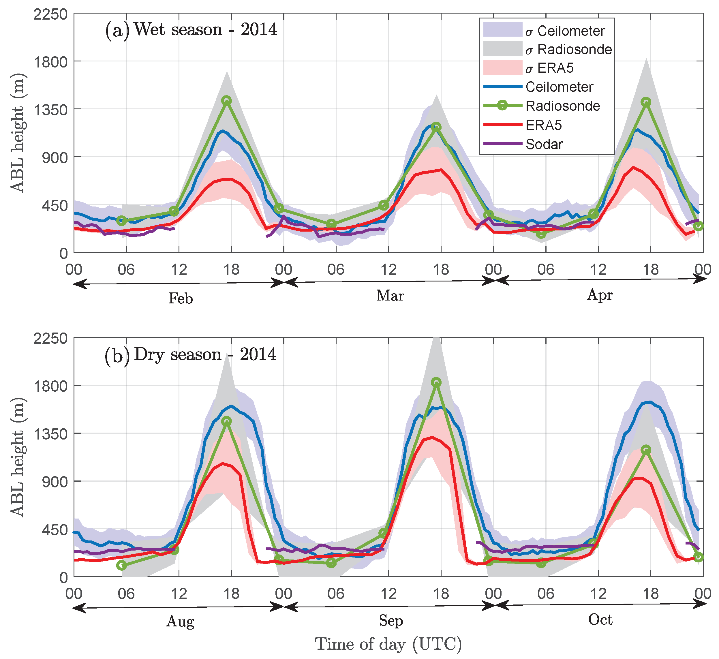
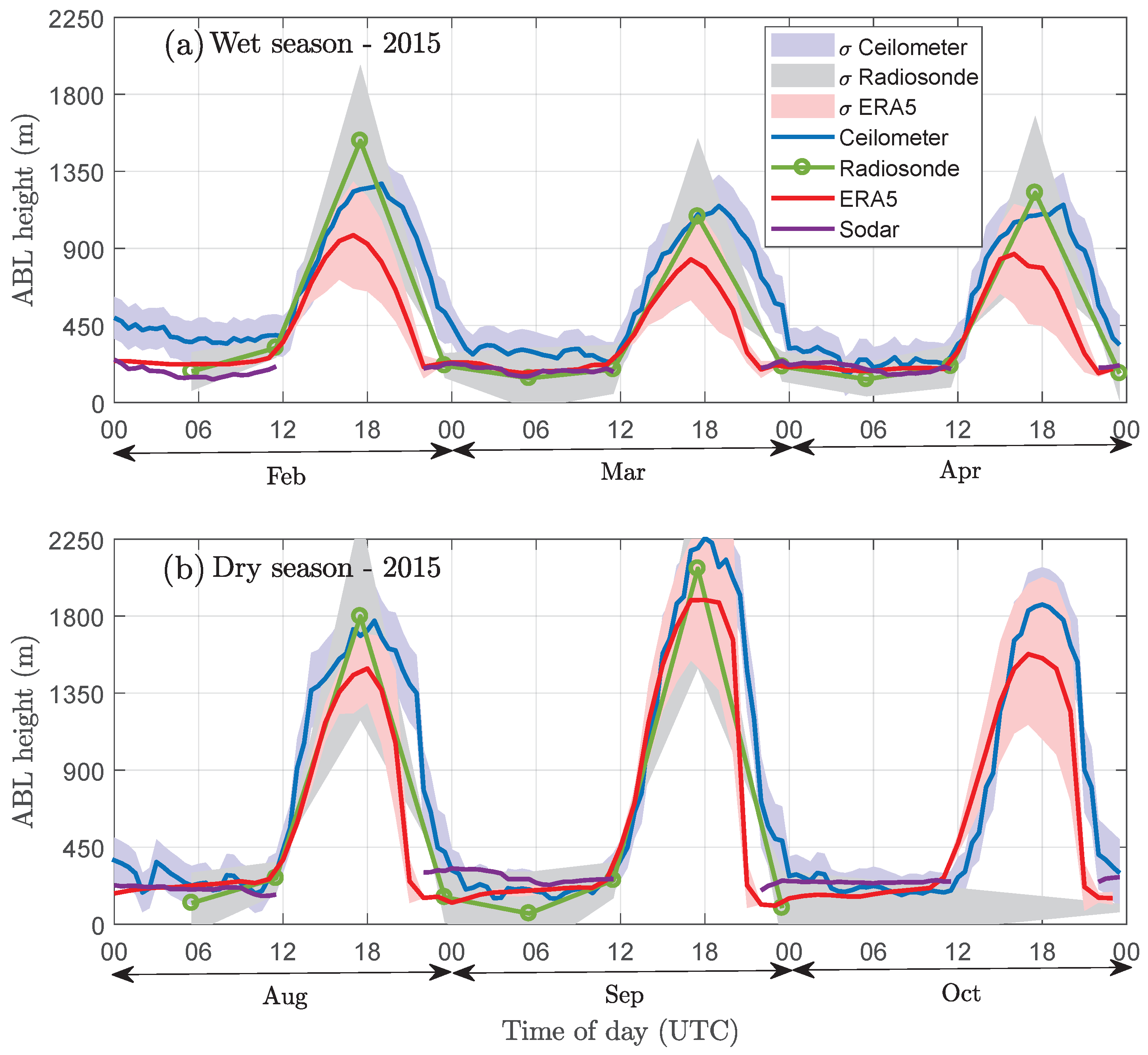
The values at the T3 site obtained by different instruments and by ERA5 estimates during the wet (Figure 2a and Figure 3a) and dry (Figure 2b and Figure 3b) seasons of 2014 (Figure 2) and 2015 (Figure 3) are shown. We can see a clear seasonal change in values for both years that is well captured by both ERA5 and the observations. This seasonality is due to the rainfall regime in Central Amazonia [30,33]. From the experimental data for 2014, the values during the wet season ranged between 900 and 1350 m, and during the dry season they ranged between 1350 and 2000 m. For 2015, the wet season values increased mainly in February with values close to 1350 m. For the dry season in 2015, the PBL heights were around 1800 and 2000 m. It is worthwhile to note the interannual scale mainly during the dry season. The performance of ERA5 relative to the observations seems to be better during the dry season of 2015, which was an El Niño year. In 2014, there is a clear underestimation for both wet and dry periods; this is also the case for the wet season of 2015. In Section 3.3, we present a physical explanation for this behavior.
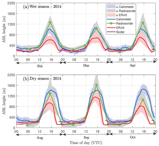
Figure 2.
Average daily cycle (data from entire month) of the PBL height at the T3 site near Manaus during the wet (a) and dry seasons (b) in 2014, derived from ceilometer (blue), SODAR (lilac), and radiosonde (green), as well as ERA5 retrieval (red). 2014 was a non-El Niño year. The shaded area represents the standard deviation.

Figure 3.
The same as Figure 2 for the El Niño-affected year 2015, during the wet (a) and dry seasons (b).
With respect to the diurnal change (Figure 2 and Figure 3), we can still see that is higher during the dry season, for both years. This behavior is well captured by ERA5, and is very close to the observed sounding values. The slope of the PBL growth is very similar between the ERA5 and the observed one. During the decreasing stage at afternoon times, ERA5 tends to anticipate its collapse in relation to the observations, especially during the dry season.
3.2. PBL Heights at the ATTO Site from In Situ Measurements and ERA5 Data
Figure 4 shows all values (derived from ERA5 and measured by a ceilometer and radiosonde) for November 2015. This is the only month with ceilometer and radiosonde data available at the ATTO site for this study. The in situ observations agreed well between them, with maximum values ranging from 1550 m (measured by ceilometer) and 1400 m (derived from radiosondes). These values were lower than the same values for the T3 site (approximately 1800 m; Figure 3b). However, this result is expected as the latter has a higher fraction of pasture, which is almost absent at and around ATTO (Table 1). This same result was demonstrated by [30] for forested and deforested areas in Rondonia State (southwest Amazonia). They showed that the sensible heat flux is higher at a pasture than at a forest site and, consequently, is also higher over deforested areas.
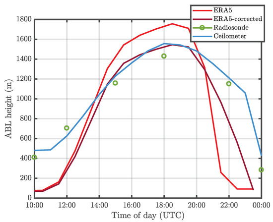
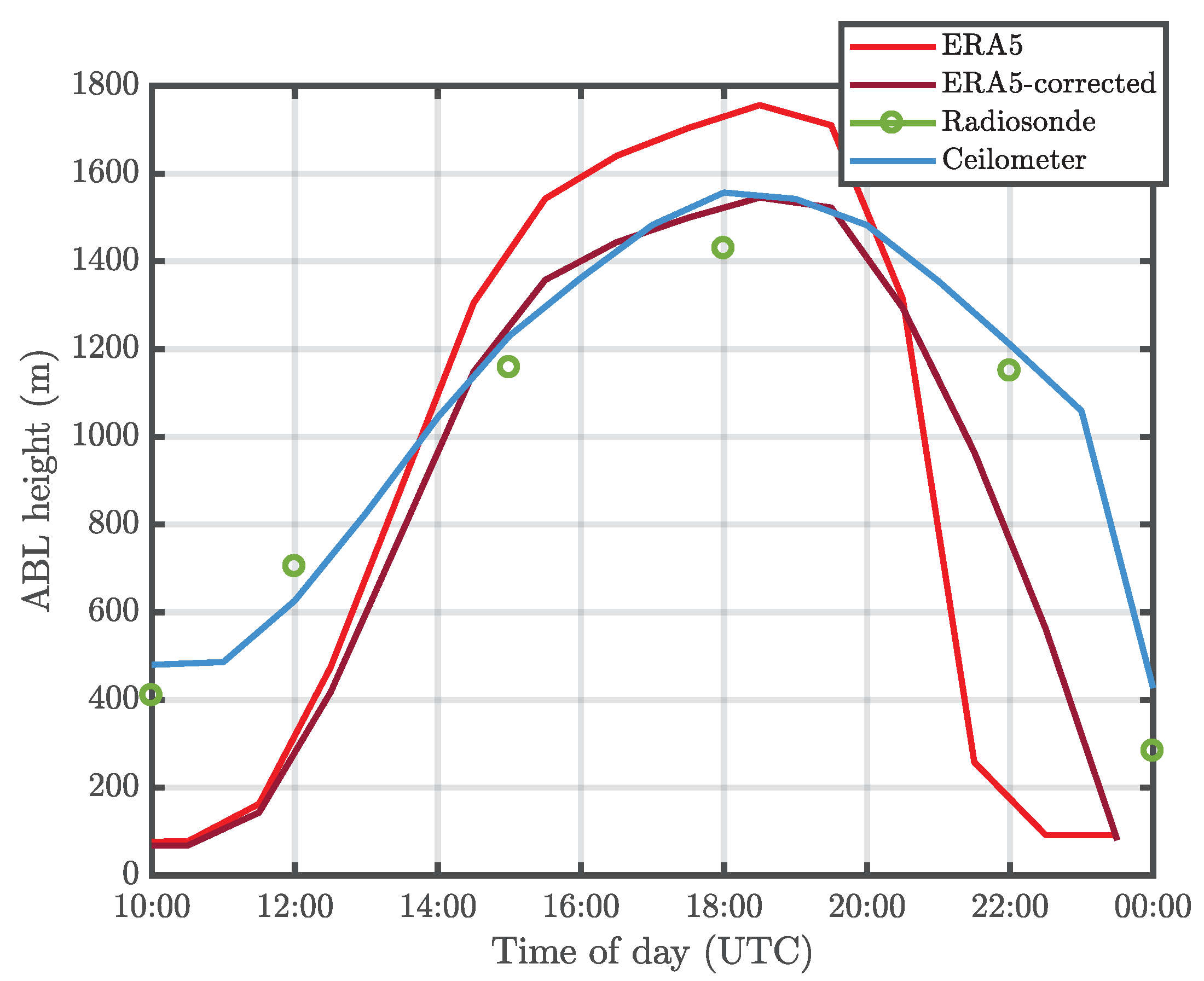
Figure 4.
Average diurnal cycle of the PBL height at ATTO in Nov 2015, obtained from ceilometer (blue) and radiosonde (green, circles, corresponding to the average of the period from 1–6 November) measurements, as well as ERA5 retrievals (red). The corrected ERA5 data (dark red) are shown for comparison, as discussed in detail in Section 3.3.
In contrast to the T3 results (Section 3.1), we found that -ERA5 overestimates the measured at ATTO, with maximum PBL heights of about 1800 m. However, the ATTO site also presented a collapsed CBL in late afternoon, which is discussed in Section 3.3.
3.3. Physical Explanations for Underestimated or Overestimated ERA5 Values
In this section, we provide the potential physical reasons for the observed overestimation of the -ERA5 values for ATTO and underestimation for T3. We believe that the main reasons are associated with the parameterization used by the model related to the sensible heat flux (H) and the atmospheric stability (given by the Richardson number, ). These parameters are shown for both sites in Figure 5, Figure 6, Figure 7 and Figure 8. The H experimental values at both sites (T3 and ATTO) were determined by the eddy covariance (EC) technique, measured by a 3D sonic anemometer. Note that the H values simulated by ERA5 were higher than the ones obtained experimentally for both the T3 and ATTO sites (Figure 5 and Figure 8, respectively). This means that the ERA5 is computing higher sensible heat fluxes for the Central Amazonian. The height of the convective boundary layer is strongly dependent on the surface heat fluxes.
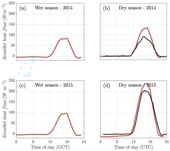
Figure 5.
Sensible heat flux values through experimental data (black line) and ERA5 (red line) at the T3 site. The data correspond to the wet seasons of (a,c) 2014 and 2015, and the dry seasons of (b,d) 2014 and 2015.
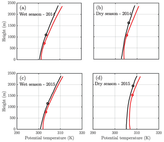
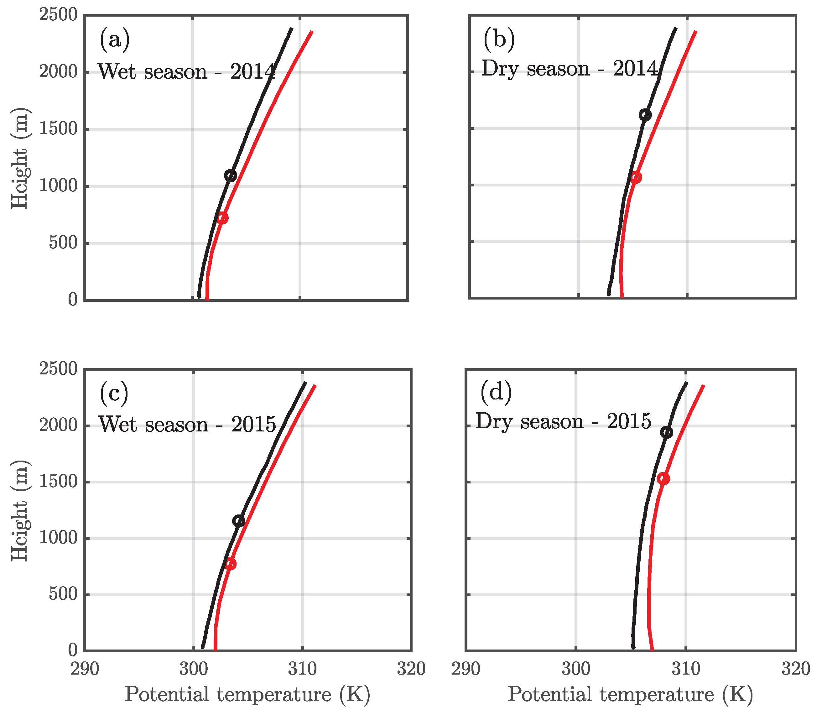
Figure 6.
Potential temperature profile from experimental data (black line) and ERA5 (red line) at the T3 site. The data correspond to the wet seasons of (a,c) 2014 and 2015 and the dry seasons of (b,d) 2014 and 2015. The vertical profiles for both ERA5 and experimental data represent an average of all profiles made at 18:00 UTC (14:00 LT). The black and red circles correspond to the average height of the boundary layer estimated through experimental data and ERA5, respectively.
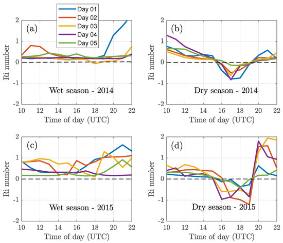
Figure 7.
values obtained through the potential temperature and wind profiles from ERA5 for the T3 site. The data correspond to the wet seasons of (a,c) 2014 and 2015 and the dry seasons of (b,d) 2014 and 2015.
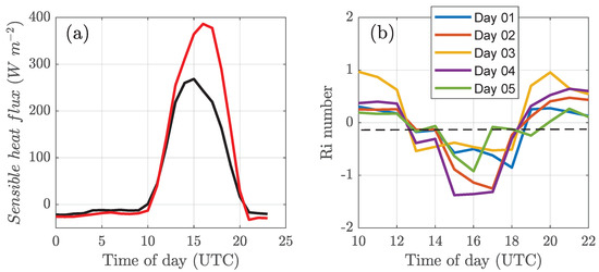
Figure 8.
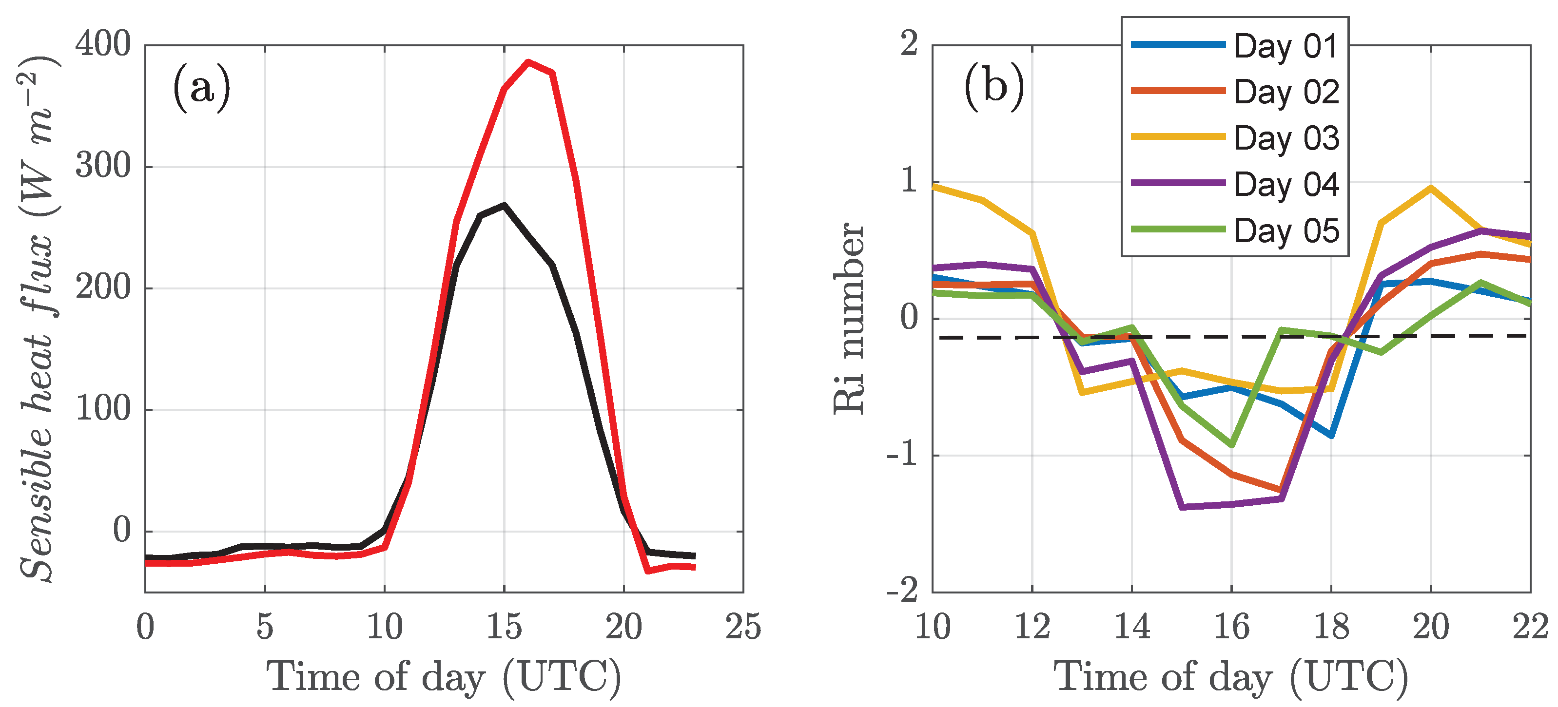
(a) Sensible heat flux values through experimental data (red line) and ERA5 (black line), and (b) values obtained through the temperature and wind profiles from ERA5 for the ATTO site. The data correspond to November 2015.
Figure 6 shows the temperature vertical profiles for both ERA5 and experimental data. The profiles correspond to an average of all profiles at 18 UTC (14 LT). This time was chosen to represent the maximum depth of the convective PBL. It is possible to note that the temperature values of the ERA5 profile were higher than the values obtained experimentally. This is associated with the high surface sensible heat flux of the ERA5 (Figure 5). However, it is interesting to note that even with higher H values, the -ERA5 was lower than the from experimental data. The apparent controversy (higher H at surface and lower depth) for ERA5 is due to the fact that the model was not able to vertically distribute all this heat released from the surface.
Previous studies have already shown that the differences between -ERA5 and from experimental data can be caused by several factors. Among them, the surface heterogeneity plays an important role in this difference [28,51], since ERA5 has difficulties in representing the surface heterogeneity, due to its relatively sparse grid. It is worth noticing that the T3 site has considerable horizontal heterogeneity (Table 1). Additionally, in work by [28], it was shown that the greatest differences between -ERA5 and from experimental data occurred in regions of low and medium latitudes, such as the sites shown in this study. In these regions, the thermal convection is strong, that is, static stability is supposed to exert an important influence on the comparison results. Ref. [28] analyzed this influence on the differences between from experimental data and -ERA5. They found that the -ERA5 values were underestimated due to an inadequate parameterization of the intensity of atmospheric instability in the lower troposphere, which does not ideally portray turbulent transport in that region. Additionally, according to [28], the afternoon values are the ones that suffer the highest errors due to inadequate mixing of air between PBL and the free atmosphere in the models, similar to that observed in this work (Figure 2 and Figure 3).
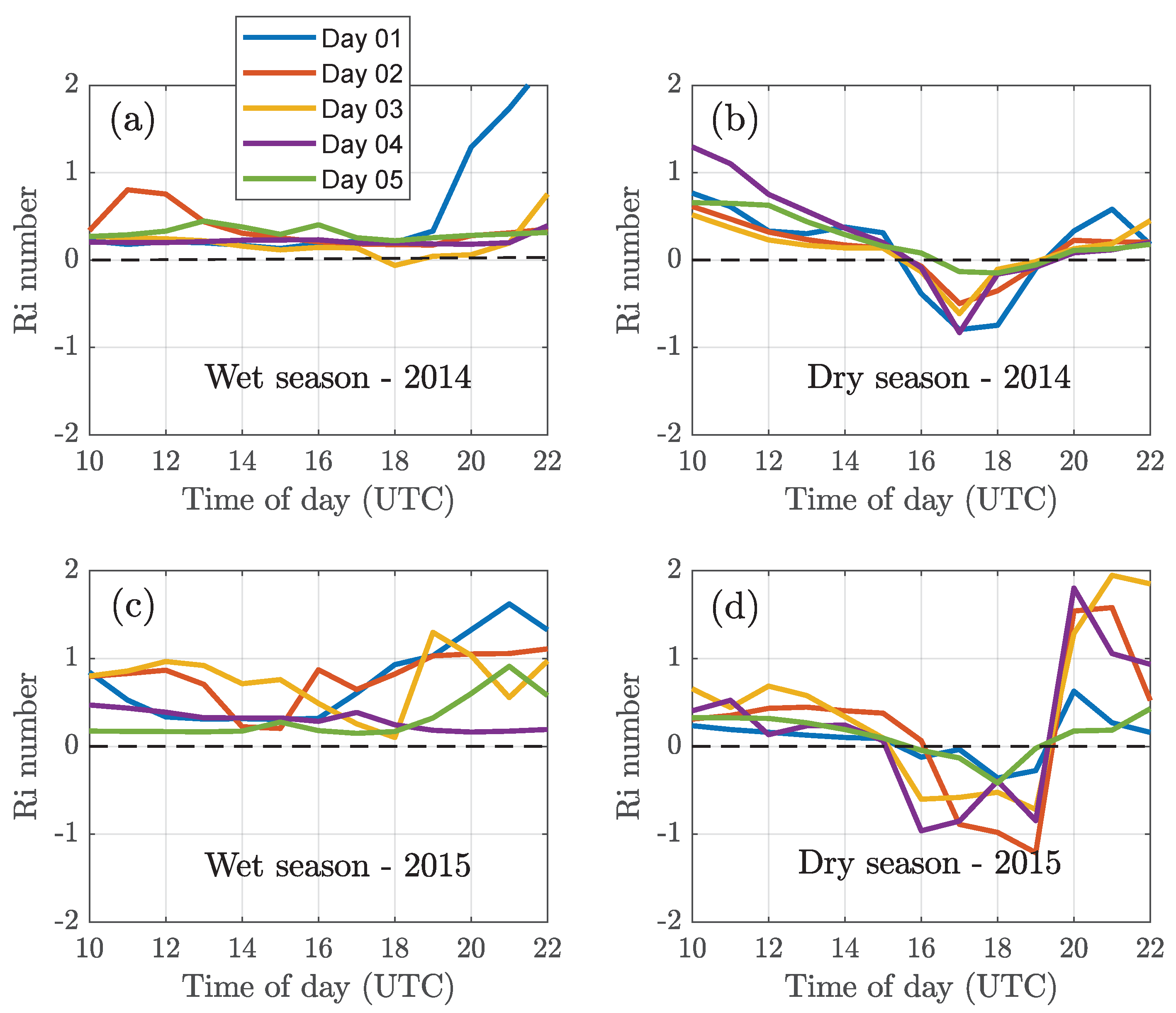
With this information in mind, Figure 7 shows the values calculated for some days of the wet season and the dry season above the T3 site. During both wet seasons (2014 and 2015), the values are always positive, indicating a stable layer, that is, the temperature at the highest level is higher than the temperature near the surface, which does not help the thermal convection mixture in this layer. For the dry season, values show differences between 2014 and 2015. For the dry season of 2014, it is around from 15:30 up to 19:00 UTC (which is from 11:30 up to 15:00 LT) and it reverses its signal (to be positive values) afterwards. Thus, the CBL is generated only for a fraction of the day (until midday). For the year 2015, which was drier, the H is higher in relation to 2014 (Figure 5) and the same behavior happens, although the is stronger (around −1.0) and weakly longer (from 15:00 until 19:30 UTC).
For the ATTO site, the difference between the H values from ERA5 and experimental data was considerably greater than for the T3 site (Figure 8a). Furthermore, for the ATTO site, (Figure 8b) is negative (around −1.5) from 12:30 until 19:00 UTC, provoking an overestimation of PBL heights. After 15:00 UTC, there is a signal reversal and becomes positive, so there is this sharp drop in -ERA5 values (Figure 4). It is believed that the higher sensible heat flux and the stronger thermal instability caused ERA5 to overestimate the values for the ATTO site, and this may be associated with the land use/cover shown in Table 1. It is possible that the presence of a reasonable fraction of water/rivers in the ERA5 grid for the T3 site produces considerable thermal stability within the simulated PBL. As for the ATTO site, the absence of water in the ERA5 grid produces the opposite effect.
3.4. ERA5 Correction for Daytime Period at the T3 and ATTO Sites
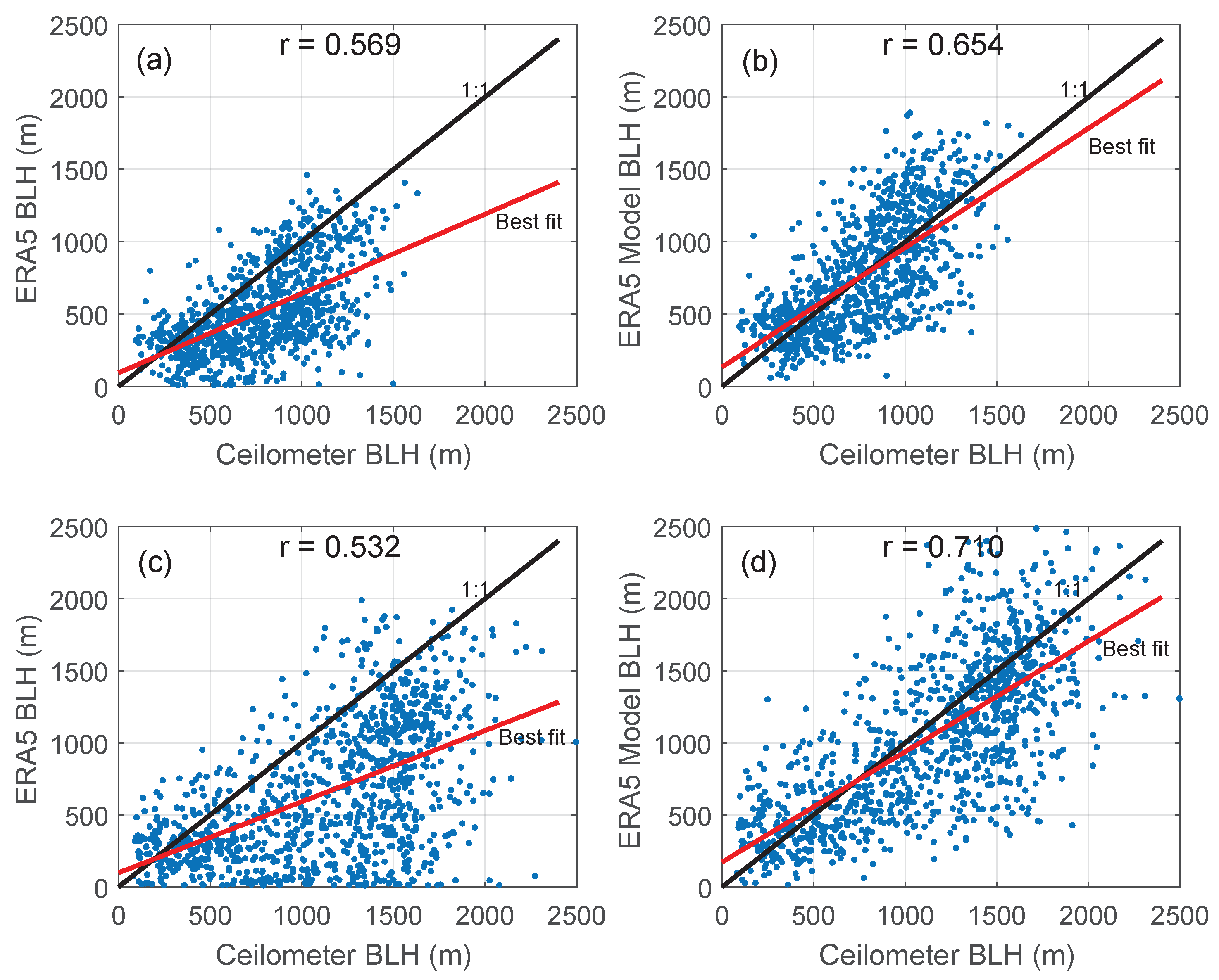
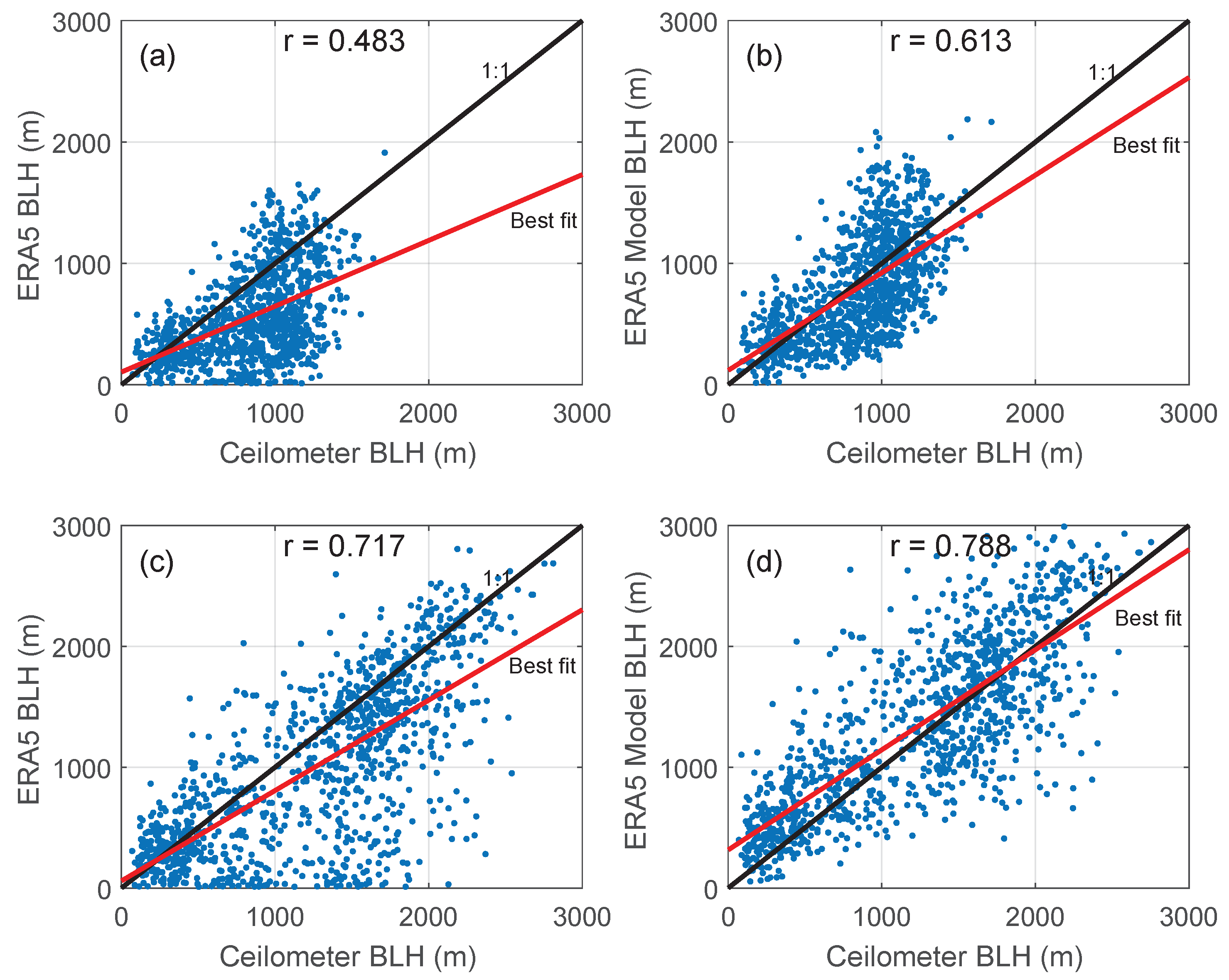
In order to determine the best correction to be applied to the -ERA5 values, a linear regression was applied using the ERA5 and the ceilometer data. The ceilometer was chosen as the best estimator of , according to [33]. This linear regression was made for the years 2014 and 2015, splitting the data available for wet (Figure 9a and Figure 10a) and dry (Figure 9c and Figure 10c) periods. The values derived from ERA5 are lower than from the observations so the slope of the best line adjusted is lower than the 1:1 line. One point that should be observed is the early reduction of the -ERA5 values in the late afternoon (similar to those observed in Figure 2 and Figure 3), associated with an early extinction of the turbulence within the daytime PBL. This may be caused by the method used in ERA5 to compute (potential temperature gradient) that is almost null at this time but the turbulence/convection is still active.
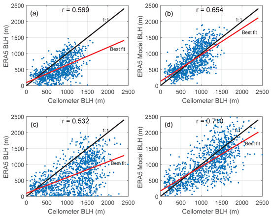
Figure 9.
Scatterplots of daytime PBL heights derived from observational data (ceilometer) and model (ERA5) for before (a,c) and after correction (b,d) for wet (a,b) and dry (c,d) seasons for the year 2014 at the T3 site.
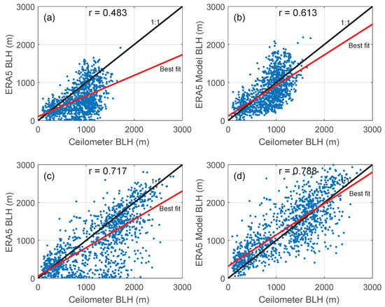
Figure 10.
Similar to Figure 9 for the year 2015: PBL heights derived from observational data (ceilometer) and model (ERA5) for before (a,c) and after correction (b,d) for wet (a,b) and dry (c,d) seasons.
For the values from ERA5 (), two procedures were adopted: (i) a coefficient () associated with an under/overestimation relative to the observations () was found (Equation (1)); (ii) Equation (2) was used to correct the PBL heights derived from ERA5 (). A sinusoidal function was chosen to correct the early reduction of the PBL heights derived from ERA5 in the late afternoon.
where corresponds to the time window of the diurnal cycle (half sinusoidal wave = 12 h). is the maximum value of on that day. The alpha values were for the year 2014 for 2015.
After the corrections were applied (Equations (1) and (2)), not only did the correlation coefficient and the slope improve, but so did the collapse of the PBL height in the late afternoon for both seasons and years.
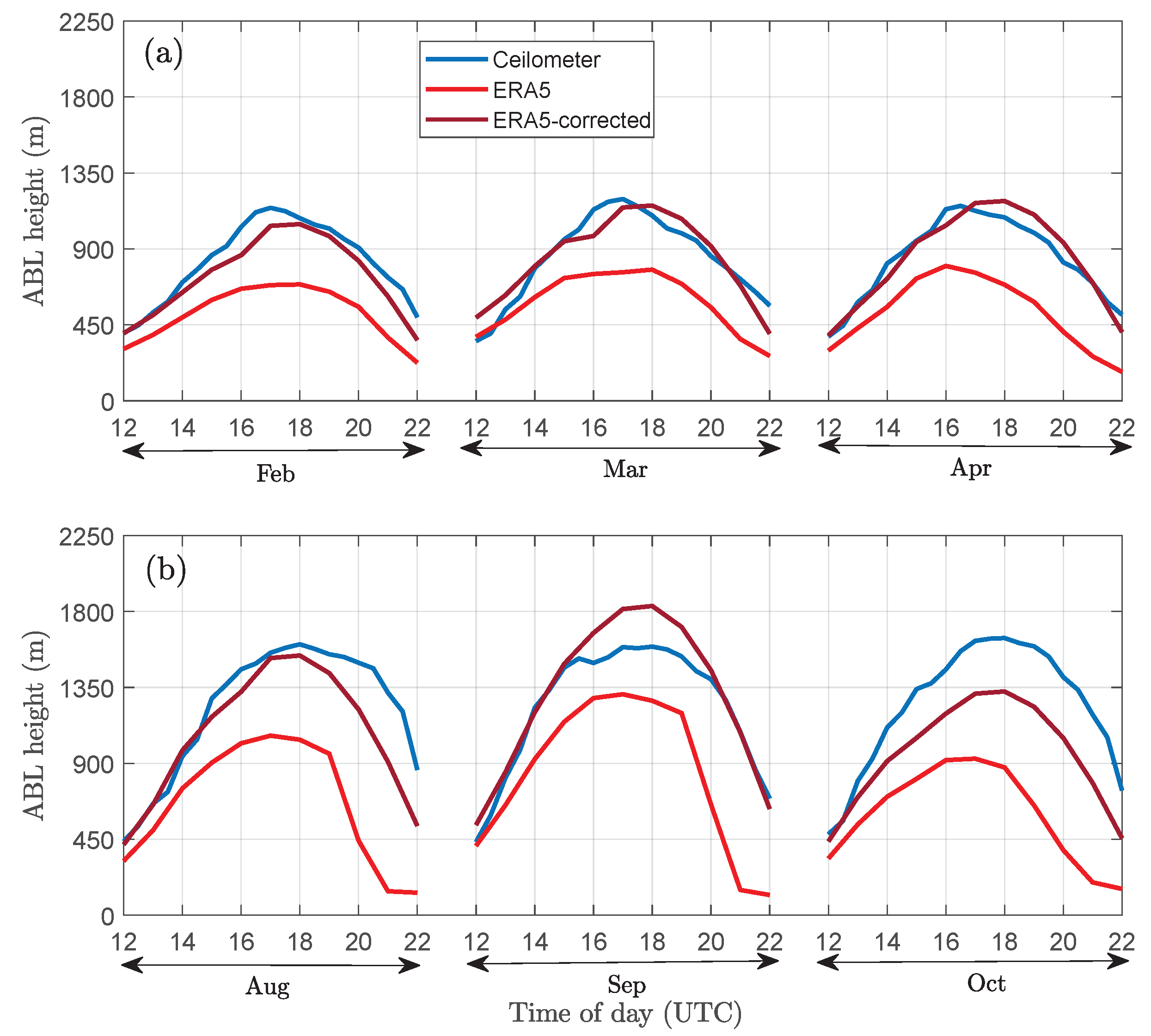
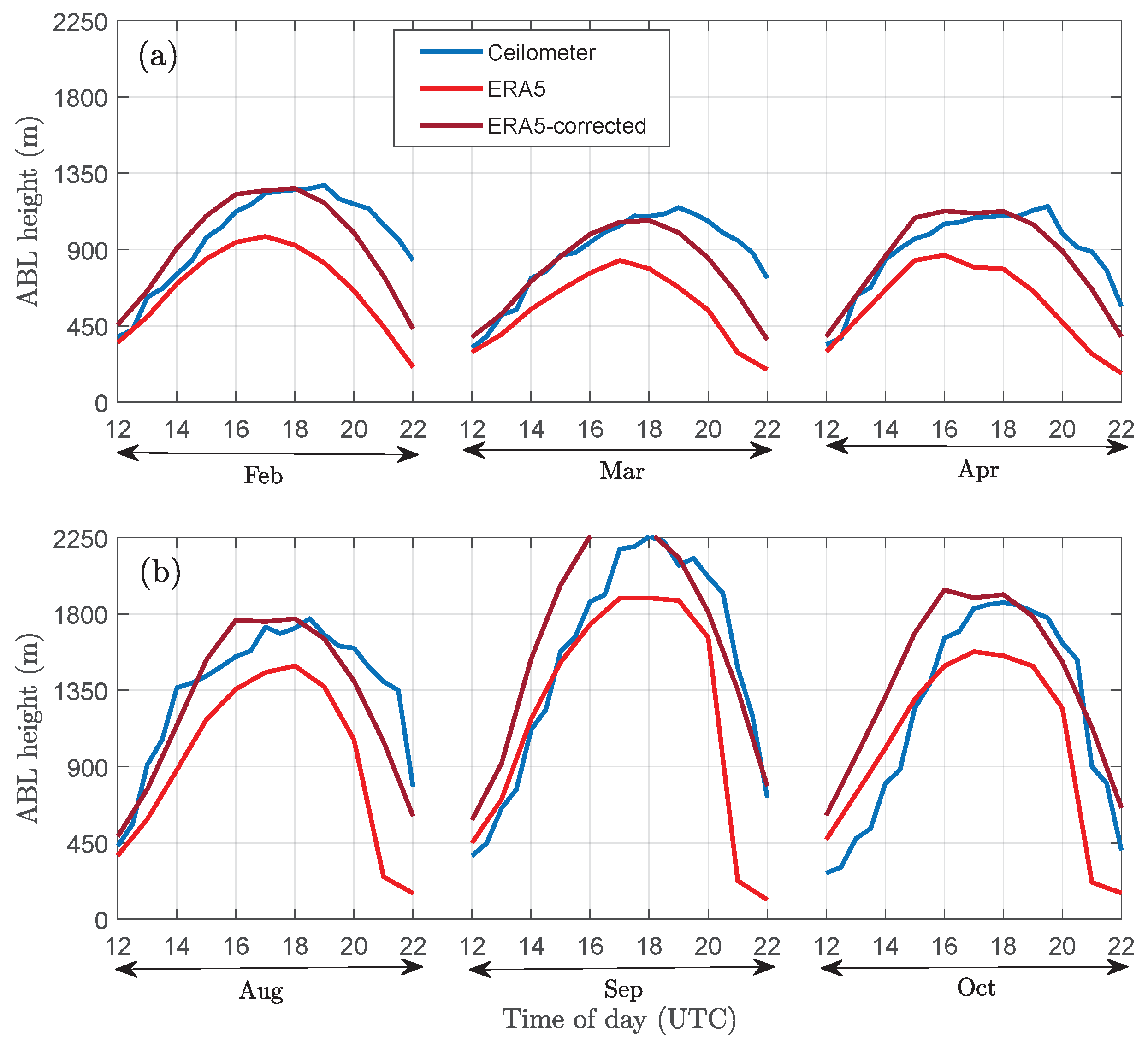
Figure 11 and Figure 12 present all values (observations, ERA5, and ERA5-corrected) for daytime. It was possible to observe that the corrections improved the diurnal cycle, especially for the wet season. For the dry season of 2014, the observations are slightly overestimated but the agreement was better than the original zi-ERA5.
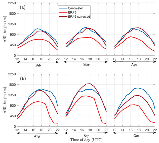
Figure 11.
Average diurnal cycle (data from entire month) for the convective PBL estimated for different instruments: ceilometer (blue line), ERA5 (red line), and ERA5-corrected (Equation (2)) for the wet (a) and dry (b) seasons for 2014 (non-El Niño year).
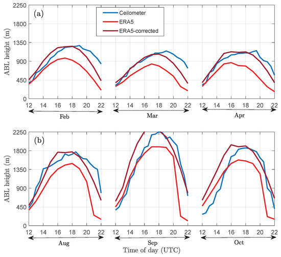
Figure 12.
Average diurnal cycle (data from entire month) for the convective PBL estimated for different instruments: ceilometer (blue line), ERA5 (red line), and ERA5-corrected (Equation (2)) for the wet (a) and dry (b) seasons for 2015 (El Niño year).
The same type of corrections for the daytime zi-ERA5 at T3 were also carried out for ATTO (Equations (1) and (2)), but was estimated to be = −0.12 (Equation (1)). After the correction, there was a better agreement between the ERA5-corrected and the observations related to the radiosondes and ceilometer estimates (Figure 4; dark red line). The earlier collapse of the CBL was quite toned down with the corrections.
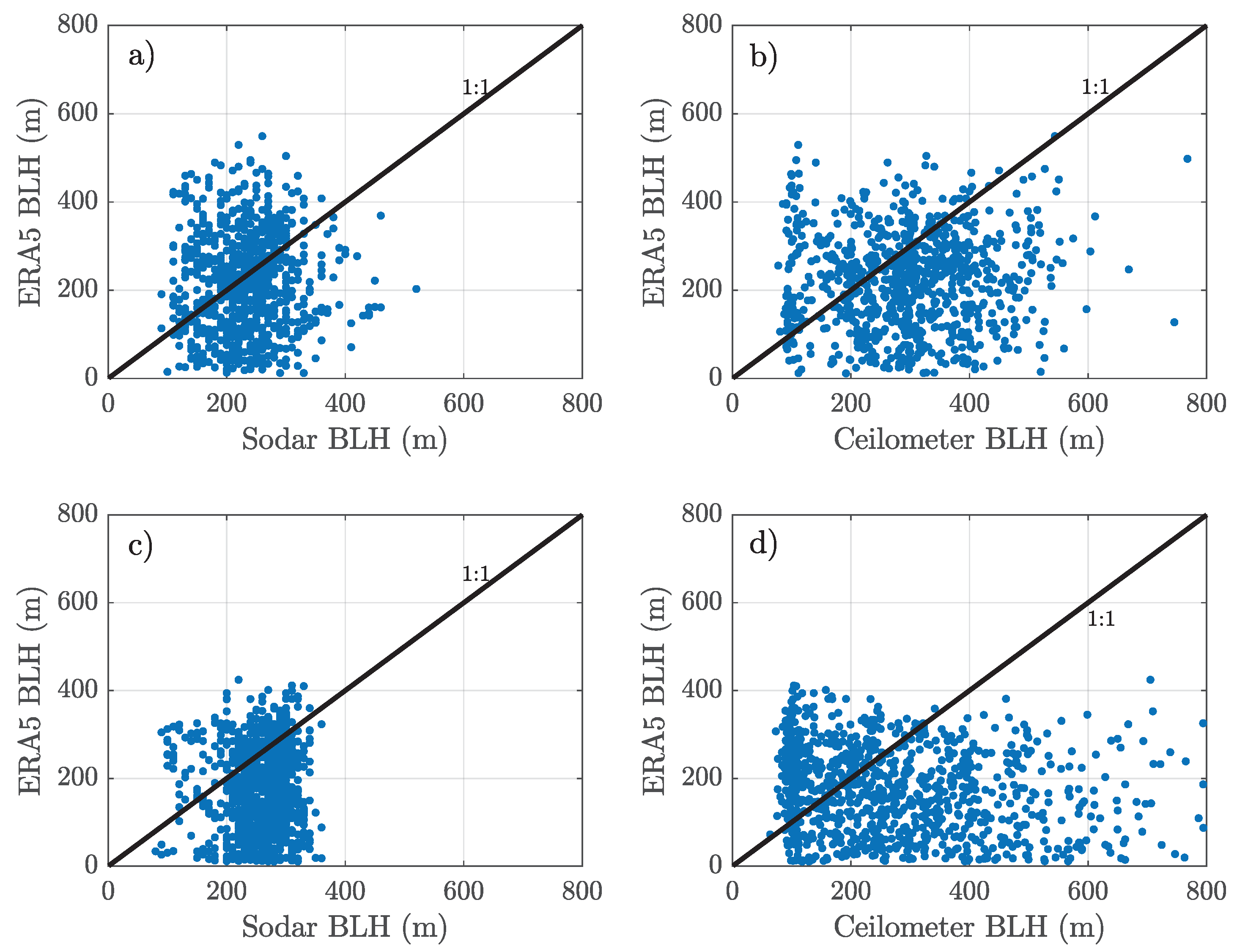
3.5. ERA5 ABL Heights for Nocturnal Periods at the T3 Site
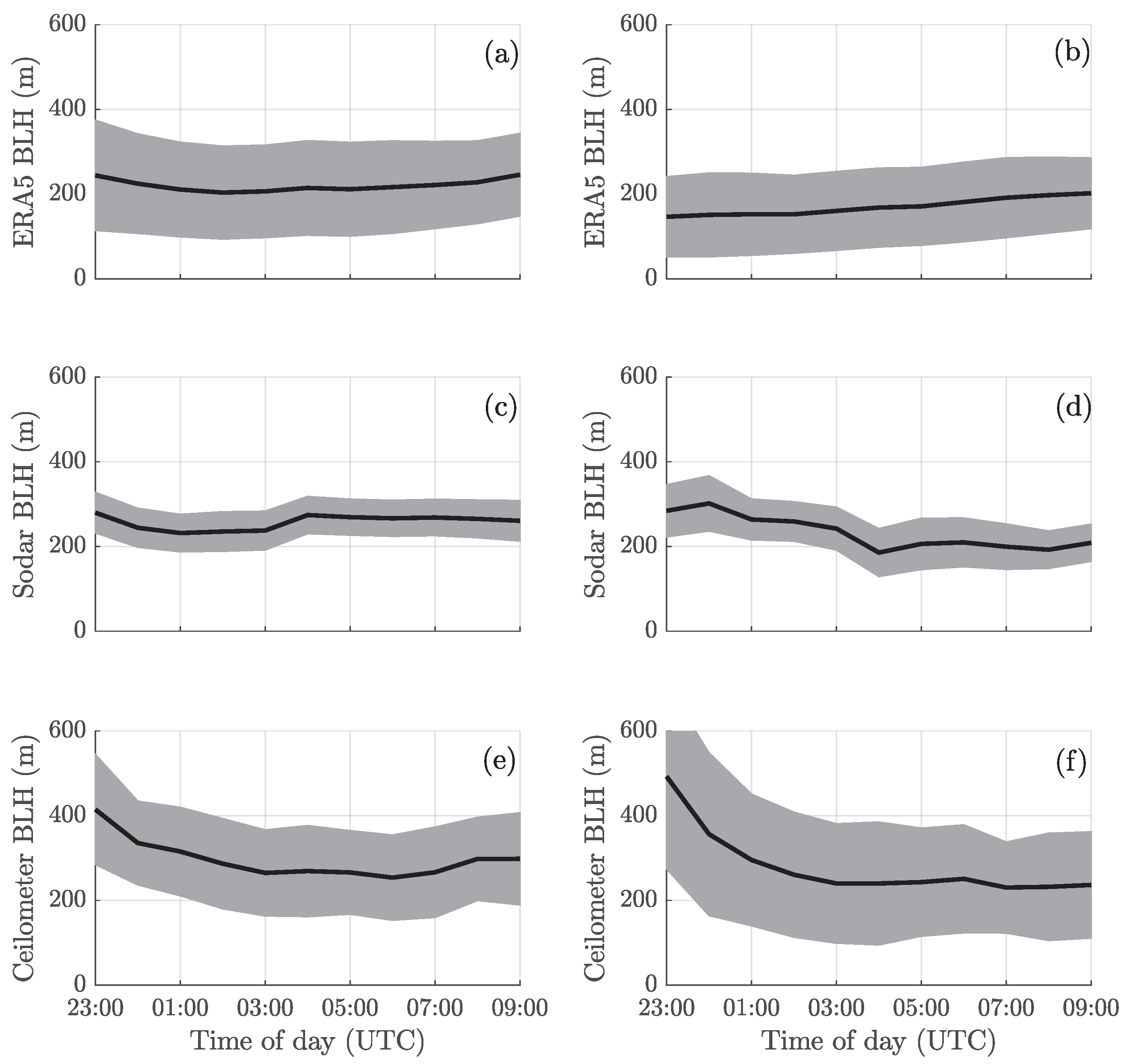
For the nocturnal period of PBL (NBL), a similar procedure to the one applied to the diurnal phase was performed, applying a linear regression during the dry and wet seasons of 2014 (Figure 13), between the -ERA5 versus -ceilometer (Figure 13b,d) and -SODAR (Figure 13a,c) values, since the SODAR also presents accurate NBL measurements [33]. Note that there is no significant relationship between -ERA5 and values obtained with experimental data and, consequently, a possible correction of -ERA5, as performed for the daytime period, becomes unlikely. The same behavior was observed for the night period of the year 2015 (not shown here). All estimates (ERA5, ceilometer, and SODAR) showed values around 250 m, with very small temporal variability during the night (Figure 14). Sometimes, the ceilometer showed values around 400–500 m (Figure 14e,f) which are not the depth of NBL, but instead arethe residual layer, following [42]. This happens as the turbulence intensity is reduced at night, making the ceilometer measurements very difficult [52].

Figure 13.
Linear regression between the -ERA5 against (a) -SODAR and (b) -ceilometer for the wet season and -ERA5 against (c) -SODAR and (d) -ceilometer for the dry season, during the nocturnal period of 2014.
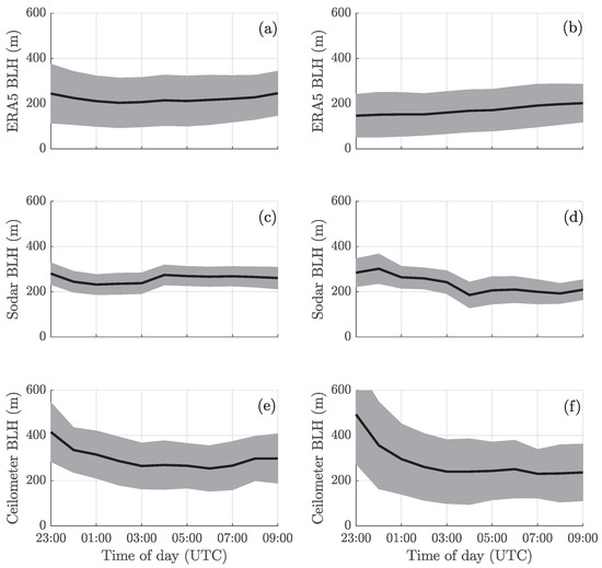
Figure 14.
Time series of the nocturnal boundary layer of -ERA5 (a,b), -SODAR (c,d), and -ceilometer (e,f) for the wet and dry seasons of 2014, respectively. The solid line is the mean value and the grey shaded area represents one standard deviation.
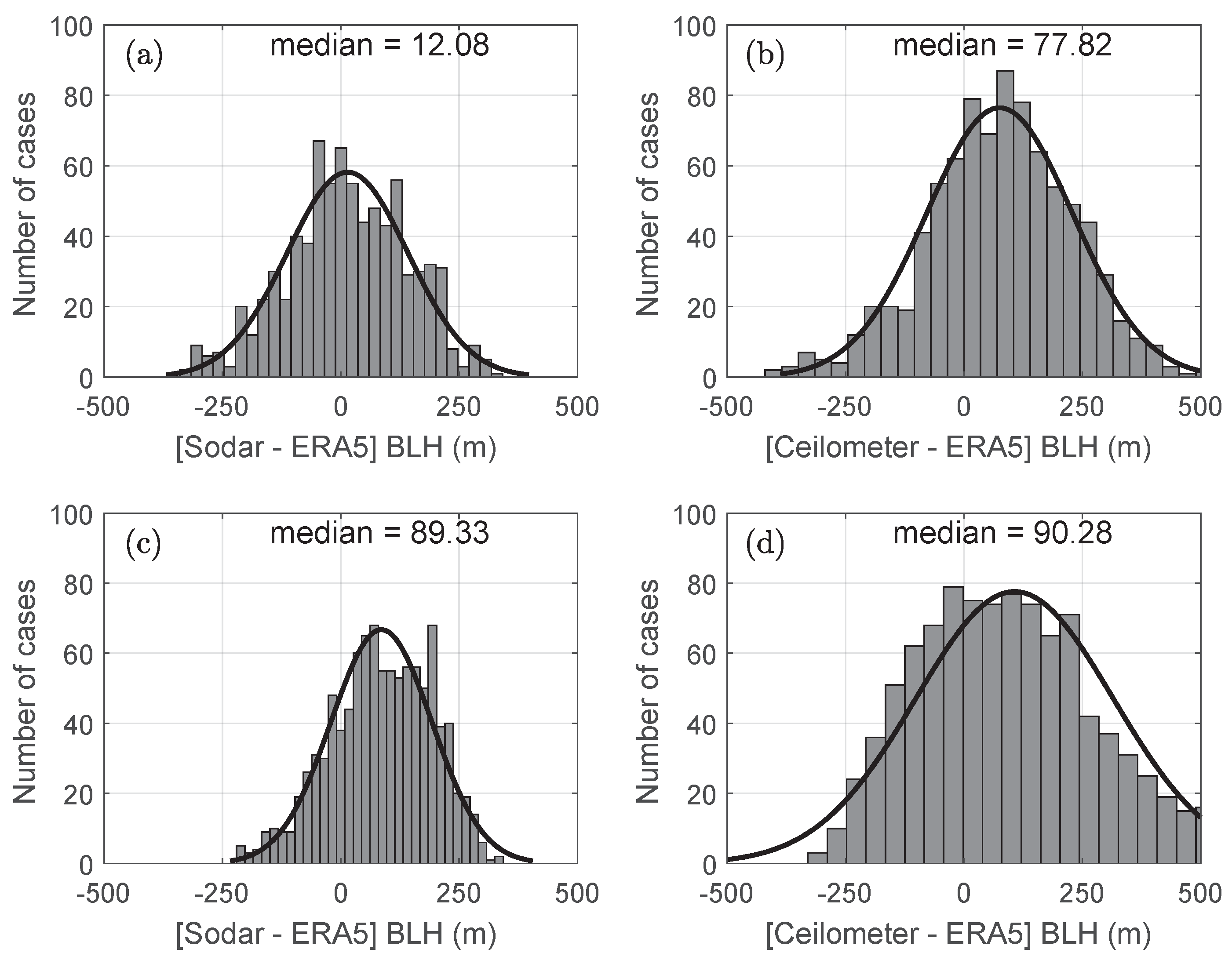
Figure 15 shows a normal (Gaussian) distribution of the differences between ERA5 and SODAR (Figure 15a,c) and ERA5 and ceilometer (Figure 15b,d). It can be noticed that the errors are well distributed along the zero values, and this is a signal that ERA5 gives a good estimate of the NBL heights. The differences were about 80–90 m for the ceilometer and ranged from 10–90 m for the SODAR. In other words, the from ERA5 underestimates (around than 90 m) the observations. The same plots from Figure 14 and Figure 15 were made for 2015 (not presented) and the results were the same.
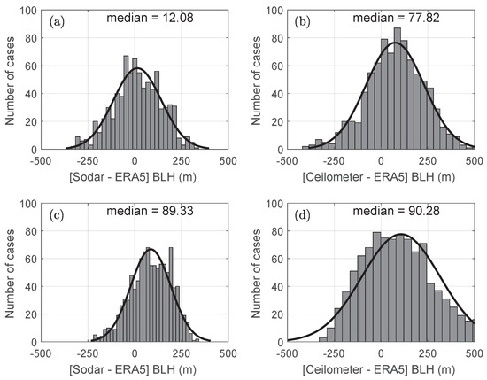
Figure 15.
Normal distribution of the differences between -ERA5 and -SODAR for (a) wet season and (c) dry season of 2014. Normal distribution of the differences between -ERA5 and -ceilometer for (b) wet season and (d) dry season of 2014.
4. Conclusions
This paper presents the first attempt to validate and correct the height of the PBL from ERA5 in Central Amazonian. A new methodology to correct the hourly PBL heights from ERA5 was proposed. The major correction identified is the early reduction of its height in the late afternoon that is not physically reasonable. Probably this is due to not considering the entrainment fluxes contribution to maintain the turbulence at this period. Additionally, due to the heterogeneity of the surface, the values derived from ERA5 are higher than the observations during daytime periods above the forest area (ATTO site), and are always smaller above the forest–pasture–river area (T3 site). Additionally, after the correction of the hourly values of the height of the PBL from ERA5, we obtained a better correlation between the experimental data and ERA5, for both forest and forest–pasture–river areas and for both years: typical and El Niño year.
The ERA5 values did not develop a real thermal stratification when compared with observations. This may be due to the parametrization of H and for the PBL, especially during daytime. Additionally, there is the influence of the heterogeneity of the surface, as the model considered tropical forest, and in fact there is a mixture of different biomass (forest, pasture, and water).
The NBL heights derived from ERA5 were similarly (without any shift or trend) related to the observations (SODAR and Ceilometer). Thus, the outputs of the NBL from ERA5 can be used as typical values, for both seasons (wet and dry), for a non and El Niño year. However, as they present a higher variability they cannot be used at hourly time periods. Based on the analysis performed and expertise gained for nighttime PBL, it should be desirable to conduct new fieldwork in order to validate and calibrate models. The ATTO’s tower (325 m height) is a suitable platform to understand the behavior of the NBL and its erosion as there is a profile of climatic elements (such as temperature, humidity, winds) and turbulent fluxes (such as H). The analysis of all these data with 3D simulations using a very-high-resolution model (such as LES) will permit a better understanding of the NBL.
For the first time, comparisons of the PBL height estimates obtained experimentally with those from the ERA5 reanalysis for the Amazon region are presented. Although the correction/validation proposed in this work was performed using empirical analysis, it can be used in other areas of the Amazonia with similar climate/land use characteristics of the GoAmazon and ATTO sites, if there are no experimental data available. Additionally, it is useful for ongoing and future research that would like to use PBL heights derived from ERA5 for the GoAmazon and ATTO region, and may benefit the scientific community that is working with the coupling between the Amazonia vegetation and atmosphere.
Author Contributions
Conceptualization, C.Q.D.-J., R.G.C., G.F. and M.S.; methodology, C.Q.D.-J., R.G.C. and G.F.; software, C.Q.D.-J. and R.G.C.; validation, C.Q.D.-J. and R.G.C.; formal analysis, C.Q.D.-J., R.G.C., G.F., M.S., F.A.F.D. and S.B.; investigation, C.Q.D.-J., R.G.C. and G.F.; data curation, S.W. and R.M.N.d.S.; writing—original draft preparation, C.Q.D.-J., R.G.C., G.F., S.B., L.A.T.M. and C.P. All authors have read and agreed to the published version of the manuscript.
Funding
This research received no external funding.
Data Availability Statement
The datasets used in this work are available at the ARM Climate Research Facility database for the GoAmazon2014/5 experiment (https://www.arm.gov/research/campaigns/amf2014goamazon, accessed on 1 September 2020) and in the ATTO data portal (https://www.attodata.org/, accessed on 1 September 2020).
Acknowledgments
This work was supported by the Max Planck Society as well as the Amazon State University (UEA), FAPEAM, LBA/INPA, and SDS/CEUC/RDS-Uatumã. We also thank the European Centre for Medium-Range Weather Forecasts (ECMWF) for the reanalysis data. We also would like to thank the GOAMAZON Project group for providing the data for this study.
Conflicts of Interest
The authors declare no conflict of interest.
References
- Garratt, J.R. The Atmospheric Boundary Layer—Cambridge Atmospheric and Space Science Series; Cambridge University Press: Cambridge, UK, 1992. [Google Scholar]
- Stull, R.B. An Introduction to Boundary Layer Meteorology; Springer Science & Business Media: Berlin/Heidelberg, Germany, 2012; Volume 13. [Google Scholar]
- Garratt, J.R. The atmospheric boundary layer. Earth-Sci. Rev. 1994, 37, 89–134. [Google Scholar] [CrossRef]
- Su, T.; Li, Z.; Kahn, R. Relationships between the planetary boundary layer height and surface pollutants derived from lidar observations over China: Regional pattern and influencing factors. Atmos. Chem. Phys. 2018, 18, 15921–15935. [Google Scholar] [CrossRef]
- Henkes, A.; Fisch, G.; Machado, L.A.T.; Chaboureau, J.P. Morning boundary layer conditions for shallow to deep convective cloud evolution during the dry season in the central Amazon. Atmos. Chem. Phys. 2021, 21, 13207–13225. [Google Scholar] [CrossRef]
- Seibert, P.; Beyrich, F.; Gryning, S.E.; Joffre, S.; Rasmussen, A.; Tercier, P. Review and intercomparison of operational methods for the determination of the mixing height. Atmos. Environ. 2000, 34, 1001–1027. [Google Scholar] [CrossRef]
- Hennemuth, B.; Lammert, A. Determination of the atmospheric boundary layer height from radiosonde and lidar backscatter. Bound.-Layer Meteorol. 2006, 120, 181–200. [Google Scholar] [CrossRef]
- Tucker, S.C.; Senff, C.J.; Weickmann, A.M.; Brewer, W.A.; Banta, R.M.; Sandberg, S.P.; Law, D.C.; Hardesty, R.M. Doppler lidar estimation of mixing height using turbulence, shear, and aerosol profiles. J. Atmos. Ocean. Technol. 2009, 26, 673–688. [Google Scholar] [CrossRef]
- Sawyer, V.; Li, Z. Detection, variations and intercomparison of the planetary boundary layer depth from radiosonde, lidar and infrared spectrometer. Atmos. Environ. 2013, 79, 518–528. [Google Scholar] [CrossRef]
- Beyrich, F. Mixing height estimation from sodar data—A critical discussion. Atmos. Environ. 1997, 31, 3941–3953. [Google Scholar] [CrossRef]
- Eresmaa, N.; Karppinen, A.; Joffre, S.; Räsänen, J.; Talvitie, H. Mixing height determination by ceilometer. Atmos. Chem. Phys. 2006, 6, 1485–1493. [Google Scholar] [CrossRef]
- Van der Kamp, D.; McKendry, I. Diurnal and seasonal trends in convective mixed-layer heights estimated from two years of continuous ceilometer observations in Vancouver, BC. Bound.-Layer Meteorol. 2010, 137, 459–475. [Google Scholar] [CrossRef]
- Dai, C.; Wang, Q.; Kalogiros, J.; Lenschow, D.; Gao, Z.; Zhou, M. Determining boundary-layer height from aircraft measurements. Bound.-Layer Meteorol. 2014, 152, 277–302. [Google Scholar] [CrossRef]
- Jordan, N.S.; Hoff, R.M.; Bacmeister, J.T. Validation of Goddard Earth Observing System-version 5 MERRA planetary boundary layer heights using CALIPSO. J. Geophys. Res. Atmos. 2010, 115, D24218. [Google Scholar] [CrossRef]
- Teixeira, J.; Piepmeier, J.; Nehrir, A.; Ao, C.; Chen, S.; Clayson, C.; Fridlind, A.; Lebsock, M.; McCarty, W.; Salmun, H.; et al. Toward a Global Planetary Boundary Layer Observing System: The NASA PBL Incubation Study Team Report; NASA PBL Incubation Study Team, 2021. [Google Scholar]
- Ratnam, M.; Basha, S. A robust method to determine global distribution of atmospheric boundary layer top from COSMIC GPS RO measurements. Atmos. Sci. Lett. 2010, 11, 216–222. [Google Scholar] [CrossRef]
- Guo, P.; Kuo, Y.H.; Sokolovskiy, S.; Lenschow, D. Estimating atmospheric boundary layer depth using COSMIC radio occultation data. J. Atmos. Sci. 2011, 68, 1703–1713. [Google Scholar] [CrossRef]
- McGrath-Spangler, E.L.; Denning, A.S. Estimates of North American summertime planetary boundary layer depths derived from space-borne lidar. J. Geophys. Res. Atmos. 2012, 117, D15101. [Google Scholar] [CrossRef]
- Chahine, M.T.; Pagano, T.S.; Aumann, H.H.; Atlas, R.; Barnet, C.; Blaisdell, J.; Chen, L.; Fetzer, E.J.; Goldberg, M.; Gautier, C.; et al. AIRS: Improving weather forecasting and providing new data on greenhouse gases. Bull. Am. Meteorol. Soc. 2006, 87, 911–926. [Google Scholar] [CrossRef]
- Zhang, W.; Guo, J.; Miao, Y.; Liu, H.; Zhang, Y.; Li, Z.; Zhai, P. Planetary boundary layer height from CALIOP compared to radiosonde over China. Atmos. Chem. Phys. 2016, 16, 9951–9963. [Google Scholar] [CrossRef]
- Su, T.; Li, J.; Li, C.; Xiang, P.; Lau, A.K.H.; Guo, J.; Yang, D.; Miao, Y. An intercomparison of long-term planetary boundary layer heights retrieved from CALIPSO, ground-based lidar, and radiosonde measurements over Hong Kong. J. Geophys. Res. Atmos. 2017, 122, 3929–3943. [Google Scholar] [CrossRef]
- Hersbach, H.; Bell, B.; Berrisford, P.; Hirahara, S.; Horányi, A.; Muñoz-Sabater, J.; Nicolas, J.; Peubey, C.; Radu, R.; Schepers, D.; et al. The ERA5 global reanalysis. Q. J. R. Meteorol. Soc. 2020, 146, 1999–2049. [Google Scholar] [CrossRef]
- Dee, D.P.; Uppala, S.M.; Simmons, A.; Berrisford, P.; Poli, P.; Kobayashi, S.; Andrae, U.; Balmaseda, M.; Balsamo, G.; Bauer, d.P.; et al. The ERA-Interim reanalysis: Configuration and performance of the data assimilation system. Q. J. R. Meteorol. Soc. 2011, 137, 553–597. [Google Scholar] [CrossRef]
- Allabakash, S.; Lim, S. Climatology of Planetary Boundary Layer Height-Controlling Meteorological Parameters Over the Korean Peninsula. Remote Sens. 2020, 12, 2571. [Google Scholar] [CrossRef]
- Zhang, Y.; Sun, K.; Gao, Z.; Pan, Z.; Shook, M.A.; Li, D. Diurnal climatology of planetary boundary layer height over the contiguous United States derived from AMDAR and reanalysis data. J. Geophys. Res. Atmos. 2020, 125, e2020JD032803. [Google Scholar] [CrossRef]
- Saha, S.; Sharma, S.; Kumar, K.N.; Kumar, P.; Lal, S.; Kamat, D. Investigation of Atmospheric Boundary Layer characteristics using Ceilometer Lidar, COSMIC GPS RO satellite, Radiosonde and ERA-5 reanalysis dataset over Western Indian Region. Atmos. Res. 2022, 268, 105999. [Google Scholar] [CrossRef]
- Madonna, F.; Summa, D.; Di Girolamo, P.; Marra, F.; Wang, Y.; Rosoldi, M. Assessment of Trends and Uncertainties in the Atmospheric Boundary Layer Height Estimated Using Radiosounding Observations over Europe. Atmosphere 2021, 12, 301. [Google Scholar] [CrossRef]
- Guo, J.; Zhang, J.; Yang, K.; Liao, H.; Zhang, S.; Huang, K.; Lv, Y.; Shao, J.; Yu, T.; Tong, B.; et al. Investigation of near-global daytime boundary layer height using high-resolution radiosondes: First results and comparison with ERA5, MERRA-2, JRA-55, and NCEP-2 reanalyses. Atmos. Chem. Phys. 2021, 21, 17079–17097. [Google Scholar] [CrossRef]
- Martin, C.L.; Fitzjarrald, D.; Garstang, M.; Oliveira, A.P.; Greco, S.; Browell, E. Structure and growth of the mixing layer over the Amazonian rain forest. J. Geophys. Res. Atmos. 1988, 93, 1361–1375. [Google Scholar] [CrossRef]
- Fisch, G.; Tota, J.; Machado, L.; Dias, M.S.; Lyra, R.d.F.; Nobre, C.; Dolman, A.; Gash, J. The convective boundary layer over pasture and forest in Amazonia. Theor. Appl. Climatol. 2004, 78, 47–59. [Google Scholar] [CrossRef]
- Miranda, F.; Dias-Junior, C.Q.; Souza, C.; Sá, L.D. Estimativa da Altura da Camada Limite Convectiva sobre Floresta Amazônica. Ciência e Natura 2013, 136–138. [Google Scholar] [CrossRef]
- Dias-Júnior, C.Q.; Dias, N.L.; dos Santos, R.M.N.; Sörgel, M.; Araújo, A.; Tsokankunku, A.; Ditas, F.; de Santana, R.A.; von Randow, C.; Sá, M.; et al. Is there a classical inertial sublayer over the Amazon forest? Geophys. Res. Lett. 2019, 46, 5614–5622. [Google Scholar] [CrossRef]
- Carneiro, R.G.; Fisch, G. Observational analysis of the daily cycle of the planetary boundary layer in the central Amazon during a non-El Niño year and El Niño year (GoAmazon project 2014/5). Atmos. Chem. Phys. 2020, 20, 5547–5558. [Google Scholar] [CrossRef]
- De Santana, R.A.S.; Dias-Júnior, C.Q.; Tóta, J.; da Silva, R.; do Vale, R.S.; de Andrade, A.M.D.; Tapajós, R.; Mota, B.F.; Vieira, K.A.S.; de Santana, L.P.A.S. Estimating the atmospheric boundary layer height above multiple surfaces of the amazon region. Ciência e Natura 2020, 42, 25. [Google Scholar] [CrossRef]
- Martin, S.T.; Artaxo, P.; Machado, L.A.T.; Manzi, A.O.; Souza, R.A.F.d.; Schumacher, C.; Wang, J.; Andreae, M.O.; Barbosa, H.; Fan, J.; et al. Introduction: Observations and modeling of the Green Ocean Amazon (GoAmazon2014/5). Atmos. Chem. Phys. 2016, 16, 4785–4797. [Google Scholar] [CrossRef]
- Chamecki, M.; Freire, L.S.; Dias, N.L.; Chen, B.; Dias-Junior, C.Q.; Toledo Machado, L.A.; Sörgel, M.; Tsokankunku, A.; Araújo, A.C.d. Effects of vegetation and topography on the boundary layer structure above the Amazon forest. J. Atmos. Sci. 2020, 77, 2941–2957. [Google Scholar] [CrossRef]
- Vilà-Guerau de Arellano, J.; Wang, X.; Pedruzo-Bagazgoitia, X.; Sikma, M.; Agustí-Panareda, A.; Boussetta, S.; Balsamo, G.; Machado, L.; Biscaro, T.; Gentine, P.; et al. Interactions Between the Amazonian Rainforest and Cumuli Clouds: A Large-Eddy Simulation, High-Resolution ECMWF, and Observational Intercomparison Study. J. Adv. Model. Earth Syst. 2020, 12, e2019MS001828. [Google Scholar] [CrossRef]
- Andreae, M.O.; Acevedo, O.C.; Araùjo, A.; Artaxo, P.; Barbosa, C.G.G.; Barbosa, H.M.J.; Brito, J.; Carbone, S.; Chi, X.; Cintra, B.B.L.; et al. The Amazon Tall Tower Observatory (ATTO): Overview of pilot measurements on ecosystem ecology, meteorology, trace gases, and aerosols. Atmos. Chem. Phys. 2015, 15, 10723–10776. [Google Scholar] [CrossRef]
- Corrêa, P.B.; Dias-Júnior, C.Q.; Cava, D.; Sörgel, M.; Botía, S.; Acevedo, O.; Oliveira, P.E.S.; Manzi, A.O.; Machado, L.A.T.; Martins, H.S.; et al. A case study of a gravity wave induced by Amazon forest orography and low level jet generation. Agric. For. Meteorol. 2021, 307, 108457. [Google Scholar] [CrossRef]
- Von Randow, C.; Manzi, A.O.; Kruijt, B.; De Oliveira, P.; Zanchi, F.B.; Silva, R.d.; Hodnett, M.G.; Gash, J.H.; Elbers, J.A.; Cardoso, F.L.; et al. Comparative measurements and seasonal variations in energy and carbon exchange over forest and pasture in South West Amazonia. Theor. Appl. Climatol. 2004, 78, 5–26. [Google Scholar] [CrossRef]
- Wang, W.; Gong, W.; Mao, F.; Pan, Z. An improved iterative fitting method to estimate nocturnal residual layer height. Atmosphere 2016, 7, 106. [Google Scholar] [CrossRef]
- Carneiro, R.; Fisch, G.; Neves, T.; Santos, R.; Santos, C.; Borges, C. Nocturnal Boundary Layer Erosion Analysis in the Amazon Using Large-Eddy Simulation during GoAmazon Project 2014/5. Atmosphere 2021, 12, 240. [Google Scholar] [CrossRef]
- Neves, T.T.d.A.T.; Fisch, G. Camada limite noturna sobre área de pastagem na Amazônia. Rev. Bras. Meteorol. 2011, 26, 619–628. [Google Scholar] [CrossRef] [Green Version]
- Cohn, S.A.; Angevine, W.M. Boundary layer height and entrainment zone thickness measured by lidars and wind-profiling radars. J. Appl. Meteorol. 2020, 39, 1233–1247. [Google Scholar] [CrossRef]
- Wiegner, M.; Madonna, F.; Binietoglou, I.; Forkel, R.; Gasteiger, J.; Geiß, A.; Pappalardo, G.; Schäfer, K.; Thomas, W. What is the benefit of ceilometers for aerosol remote sensing? An answer from EARLINET. Atmos. Meas. Tech. 2014, 7, 1979–1997. [Google Scholar] [CrossRef]
- Geiß, A.; Wiegner, M.; Bonn, B.; Schäfer, K.; Forkel, R.; Schneidemesser, E.V.; Münkel, C.; Chan, K.L.; Nothard, R. Mixing layer height as an indicator for urban air quality? Atmos. Meas. Tech. 2017, 10, 2969–2988. [Google Scholar] [CrossRef]
- Morris, V.R. Ceilometer Instrument Handbook; Technical report; DOE Office of Science Atmospheric Radiation Measurement (ARM) User Facility, 2016. [Google Scholar]
- Kotthaus, S.; O’Connor, E.; Münkel, C.; Charlton-Perez, C.; Haeffelin, M.; Gabey, A.M.; Grimmond, C.S.B. Recommendations for processing atmospheric attenuated backscatter profiles from Vaisala CL31 ceilometers. Atmos. Meas. Tech. 2016, 9, 3769–3791. [Google Scholar] [CrossRef]
- Geisinger, A.; Behrendt, A.; Wulfmeyer, V.; Strohbach, J.; Förstner, J.; Potthast, R. Development and application of a backscatter lidar forward operator for quantitative validation of aerosol dispersion models and future data assimilation. Atmos. Meas. Tech. 2017, 10, 4705–4726. [Google Scholar] [CrossRef]
- Uzan, L.; Egert, S.; Khain, P.; Levi, Y.; Vadislavsky, E.; Alpert, P. Ceilometers as planetary boundary layer height detectors and a corrective tool for COSMO and IFS models. Atmos. Chem. Phys. 2020, 20, 12177–12192. [Google Scholar] [CrossRef]
- Renfrew, I.A.; Barrell, C.; Elvidge, A.D.; Brooke, J.K.; Duscha, C.; King, J.C.; Kristiansen, J.; Cope, T.L.; Moore, G.W.K.; Pickart, R.S.; et al. An evaluation of surface meteorology and fluxes over the Iceland and Greenland Seas in ERA5 reanalysis: The impact of sea ice distribution. Q. J. R. Meteorol. Soc. 2021, 147, 691–712. [Google Scholar] [CrossRef]
- Kotthaus, S.; Grimmond, C.S.B. Atmospheric boundary-layer characteristics from ceilometer measurements. Part 1: A new method to track mixed layer height and classify clouds. Q. J. R. Meteorol. Soc. 2018, 144, 1525–1538. [Google Scholar] [CrossRef] [Green Version]

Publisher’s Note: MDPI stays neutral with regard to jurisdictional claims in published maps and institutional affiliations. |
© 2022 by the authors. Licensee MDPI, Basel, Switzerland. This article is an open access article distributed under the terms and conditions of the Creative Commons Attribution (CC BY) license (https://creativecommons.org/licenses/by/4.0/).