3D LiDAR Aided GNSS/INS Integration Fault Detection, Localization and Integrity Assessment in Urban Canyons

Abstract

The performance of Global Navigation Satellite System (GNSS) and Inertial Navigation System (INS) integrated navigation can be severely degraded in urban canyons due to the non-line-of-sight (NLOS) signals and multipath effects. Therefore, to achieve a high-precision and robust integrated system, real-time fault detection and localization algorithms are needed to ensure integrity. Currently, the residual chi-square test is used for fault detection in the positioning domain, but it has poor sensitivity when faults disappear. Three-dimensional (3D) light detection and ranging (LiDAR) has good positioning performance in complex environments. First, a LiDAR aided real-time fault detection algorithm is proposed. A test statistic is constructed by the mean deviation of the matched targets, and a dynamic threshold is constructed by a sliding window. Second, to solve the problem that measurement noise is estimated by prior modeling with a certain error, a LiDAR aided real-time measurement noise estimation based on adaptive filter localization algorithm is proposed according to the position deviations of matched targets. Finally, the integrity of the integrated system is assessed. The error bound of integrated positioning is innovatively verified with real test data. We conduct two experiments with a vehicle going through a viaduct and a floor hole, which, represent mid and deep urban canyons, respectively. The experimental results show that in terms of fault detection, the fault could be detected in mid urban canyons and the response time of fault disappearance is reduced by 70.24% in deep urban canyons. Thus, the poor sensitivity of the residual chi-square test for fault disappearance is improved. In terms of localization, the proposed algorithm is compared with the optimal fading factor adaptive filter (OFFAF) and the extended Kalman filter (EKF). The proposed algorithm is the most effective, and the Root Mean Square Error (RMSE) in the east and north is reduced by 12.98% and 35.1% in deep urban canyons. Regarding integrity assessment, the error bound can overbound the positioning errors in deep urban canyons relative to the EKF and the mean value of the error bounds is reduced.

1. Introduction

A reliable positioning system is the basis of autonomous driving [1]. Integrity is an important indicator for ensuring the driving safety of vehicles. The integration of the Global Satellite Navigation System (GNSS) and the Inertial Navigation System (INS) could provide real-time and high-precision positioning and this approach is widely used in military and civil fields [2,3]. However, positioning and navigation in urban canyons is still a challenge [4] because multipath GNSS signals are received due to reflection or non-line-of-sight (NLOS) signals are received due to diffraction; this eventually leads to unacceptable GNSS measurement errors [5,6,7]. The comprehensive positioning performance of the GNSS/INS integrated navigation system is seriously degraded. Therefore, to meet the positioning performance requirements in urban canyons, such as viaducts, floor holes and tunnels, the real-time detection of GNSS/INS integrated system positioning performance is essential. However, in urban canyons, there are a lot of satellites affected by NLOS and multipath. With all four core GNSS constellations of the world in operation, the number of affected satellites is ten or more. It is difficult to detect all the affected satellites and exclude them from the localization solution by traditional algorithm such as Multiple Solution Separation (MSS). Therefore, we detect faults in the positioning domain. After faults are detected, a GNSS/INS integration algorithm can be designed based on the detection results to improve the positioning accuracy and ensure the integrity of the system.

GNSS fault detection methods are mainly divided based on whether to detect specific faulty satellites [8]. Blanch et al. only used GNSS measurement information to propose a method combining a greedy search and L1 norm minimization to detect satellites with pseudo range errors greater than 20 m that were affected by multipath and NLOS signals [9]. However, in urban canyons, rapid changes in observation satellites reduced the performance of the method. Sun et al. proposed a dynamic detection and multiple fault elimination algorithm based on pseudo range comparison [10]. Using inertial measurement unit (IMU) and GNSS pseudo range data, a parallel fault detection and exclusion scheme consisting of a sliding window and a detector was designed, which can detect multiple faulty satellites in real-time. This scheme is suitable for the tightly and loosely coupled architecture. Groves et al. proposed a likelihood-based 3D-mapping-aided (3DMA) GNSS ranging algorithm and signals, which are predicted to be non-line-of-sight (NLOS) to contribute to the position solution without explicitly computing the additional path delay due to NLOS reception, which is computationally expensive [11]. Sun et al. proposed a new measurement noise covariance update scheme, with the adaptive indicator generated from pseudo range error prediction results, for a tightly coupled GNSS/IMU navigation system in urban areas [12]. Shytermeja and Attia et al. proposed the method of using a fisheye camera to suppress NLOS signals and eliminate influenced satellites [13,14]. Fisheye images are divided into sky and non-sky regions. The GNSS fault detection can be realized by identifying GNSS satellites in the non-sky region received by the receiver. However, satellites affected by multipath signals cannot be excluded by this method. Moreover, the processing technique used for camera data is complex. Wen et al. proposed a similar approach using a real-time 3D point cloud or a sliding window map for identifying edges on the top of the given building [15,16]. Based on the relationship between the edges on the top of the building or double-decker bus and all observed satellites, the satellites influenced by the NLOS signals are detected and pseudo ranges are corrected. However, only the satellites affected by NLOS signals are detected, and the environmental conditions are highly demanding. All four of the above methods need to detect specific affected satellites and exclude them from the positioning solution. However, in urban canyons, lots of satellites are affected by NLOS and multipath signals, so it is difficult to exclude them individually. The residual chi-square test is widely used for fault detection; it constructs a fault detector via the innovation of the Kalman filter (KF) [17]. The test is performed at the positioning domain to detect whether a positioning fault is present. The algorithm is efficient and works in real-time, but the sensitivity of the residual chi-square test is poor when faults disappear. As mentioned above, although the effectiveness of the existing fault detection algorithms for detecting satellites affected by multipath and NLOS signals in complex environments has been proven, challenges remain concerning the real-time performance of dynamic applications [18,19]. Therefore, it is necessary to propose a new real-time fault detection algorithm to improve the sensitivity of the residual chi-square test to fault disappearances, and the integrity of this approach should be assessed in terms of its false alarm rate and missed detection rate. LiDAR is an important sensor in autonomous driving localization, which has good performance in ranging and perception [20]. As the cost of solid-state LiDAR decreases, LiDAR has a wider range of applications [21]. LiDAR has robust performance in building high-precision map and object detection for autonomous driving [22,23]. In this paper, we carry out fault detection algorithm aided by LiDAR.

The KF is a famous recursive algorithm for discrete linear systems and has been widely used in many fields [24]. When the given system is linear and the observed noise follows a Gaussian distribution, the KF can be proven to be optimal. However, Chang et al. pointed out that the noise probability does not obey a Gaussian distribution in practice, and it is difficult to determine the dynamic model and statistical information of the noise distribution [25]. Many scholars have studied a series of filters for non-Gaussian-distributed noise. Gordon et al. developed a particle filter (PF) to address the problem of non-Gaussian Bayesian estimation [26]. However, high-dimensional state estimation may result in a heavy computational burden. The H∞ filter was proposed for the uncertainty of measurement noise, but Rigatos pointed out that it could not solve the problem that GNSS-measured values were outliers [27]. The fading filter and adaptive filter are two widely used filters that have been proposed to solve the uncertainty of the noise distribution characteristics of dynamic systems. Chen et al. analyzed the difference between the adaptive filter and fading filter in detail. The fading filter mainly sets the weight of the state covariance matrix, while the adaptive filter mainly sets the weight of the measured noise [28]. Fagin and Sorenson proposed the fading filter algorithm in the 1960s [29]. Lee and Sun et al. proposed utilizing the fading filter method in the field of integrated navigation [30,31]. Although these methods improve the performance of the KF and the resultant positioning accuracy, many matrix multiplication and inversion operations are involved, resulting in poor practicability. Li et al. proposed a dynamic fading filter algorithm to solve problems with difficult matrix multiplication operations, greatly improving the performance of the algorithm [2]. Li et al. proposed a fading filter to defend against outliers. When a GNSS fault occurred, the innovation of the last n epochs was used to estimate the innovation of the current epoch, but the weights of the last n epochs were not considered [32]. Wang et al. developed the Sage–Husa adaptive filter, designed a sliding window and determined the covariance matrix of the current epoch based on an iterative method, but it was quite difficult to choose the window length [33]. Zhou et al. proposed a new adaptive unscented KF (N-AUKF) algorithm [34]. A covariance matching criterion was designed to judge the filtering divergence, and an adaptive weighted coefficient was applied to restrain the divergence. However, this approach requires adequate measurements. Li et al. extended this definition to Kalman filtering to detect gross errors, explained its nature and its relation with the currently adopted Chi-square variables of Kalman filtering in model and data spaces and compared them with the predictive residual statistics, starting by defining an incremental chi-square method of recursive least squares [35]. All of the above algorithms are effective in complex environments. However, the measurement noise is estimated by prior modeling with a certain error. Therefore, it is necessary to estimate the measurement noise with multi-sensor redundant measurement information.

Integrity is an important indicator of GNSS positioning in the aviation field [36]. Integrity evaluation from the GNSS to the GNSS/INS integrated positioning. Protection level is an important index of integrity monitoring, which represents the upper limit of positioning error [37]. However, in the existing research, the protection level in GNSS/INS integrated positioning is mainly based on simulation experiments [38], so it is necessary to carry out the verification protection level using the real test data. The protection level can meet the application requirement of autonomous driving.

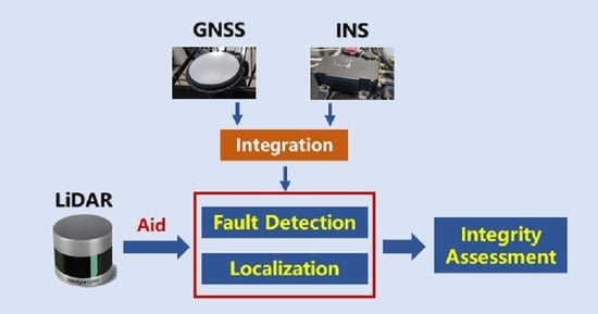
The main contributions of this paper are as follows. (1) Regarding the problem that the residual chi-square test has low sensitivity when faults disappear, a LiDAR aided real-time GNSS/INS integrated fault detection algorithm based on the characteristics of high-precision 3D LiDAR is proposed. The test statistic is constructed based on the mean position deviation of the matched targets, and the dynamic threshold is constructed by a sliding window based on the power series. (2) To solve the problem that the measurement noise is estimated by prior modeling with a certain error, a LiDAR aided measurement noise estimation and filtering algorithm is proposed. The mean position deviations of the matched targets for the last n epochs are normalized, and an adaptive weight sequence is built. The adaptive measurement noise factor is joined with the Extended Kalman Filter (EKF) innovation covariance. (3) For the problem that the integrated navigation error bounds are calculated by simulations in the existing research, we innovatively verify the error bounds of the integrated navigation system on real test data and optimize the algorithm of error bounds by using the filter in (2).

The subsequent sections of this paper are organized as follows. An overview of the proposed algorithm is given in Section 2. The proposed LiDAR aided real-time fault detection algorithm is presented in Section 3. In Section 4, the LiDAR aided measurement noise estimation adaptive filter algorithm is provided. Two experiments are performed to verify the effectiveness of the proposed algorithm, and its integrity is assessed in Section 5. Finally, Section 6 presents the conclusions and directions for future studies.

2. Overview of the Proposed Algorithm

An overview of the algorithm proposed in this paper is shown in Figure 1. First, based on LiDAR’s high-precision ranging and its perception of the surrounding environment, a LiDAR aided real-time GNSS/INS integrated positioning fault detection algorithm is proposed. A 3D LiDAR global point cloud map based on the LiDAR odometry and mapping (LOAM) [39] algorithm is established in this paper, and the map is processed in Cloud Compare software to mark the detected targets and achieve target detection. The targets in this study are mainly rods, including tree trunks and lampposts. Onboard the LiDAR, real-time scanning of the surrounding environment is carried out to detect the targets of interest based on the single frame point cloud. The targets detected based on this single frame point cloud are matched with the targets marked on the global point cloud map. A test statistic is constructed based on the mean position deviation of the matched targets, and a dynamic threshold is constructed by a sliding window based on the power series. A detector is used for the detection of GNSS/INS integrated positioning faults affected by NLOS and multipath signals. The specific implementation and detailed description of the fault detection algorithm is in Section 3.

Second, a LiDAR aided real-time measurement noise estimation adaptive filter positioning algorithm is proposed. Based on the proposed fault detection algorithm, the proposed positioning algorithm is used to improve the performance of GNSS/INS integrated positioning. The adaptive measurement noise factor is joined with the EKF innovation covariance. The mean position deviations of the matched targets for the last n epochs are normalized, and an adaptive weight sequence is built. Then, the innovation of the current epoch is calculated. Thus, the adaptive measurement noise factor for the current epoch is determined to achieve the proposed filtering and localization algorithm. The specific implementation and detailed description of the localization algorithm are in Section 4.

Finally, the integrity of the proposed algorithm is assessed based on real test data; the evaluation metrics include the missed detection and false alarm rates for fault detection and the error bounds of the localization algorithm. The integrity assessment is realized for the proposed LiDAR aided fault detection and localization algorithm under the influence of NLOS and multipath signals.

3. LiDAR Aided Real-Time Fault Detection Algorithm

3.1. KF Architecture and the Residual Chi-Square Test

3.1.1. KF Architecture

The KF is composed of state prediction and measurement update equations, as shown in Equations (1) and (2), respectively [35]. In these equations, $X_k$ represents the state vector of the system at the kth epoch, ${\Phi }_{k/k-1}$ denotes the state transition matrix of the system from the (k − 1)th epoch to the kth epoch, $W_k$ represents the system noise, $Z_k$ is the measurement vector of the system at the kth epoch, $H_k$ represents the system measurement matrix at the kth epoch, $V_k$ is the measurement noise vector and ${\Gamma }_k$ is the system noise distribution matrix.

$$X_k={\Phi }_{k/k-1}{X}_{k-1}+{\Gamma }_k{W}_k$$

(1)

$$Z_k=H_k{X}_k+V_k$$

(2)

In our research, the KF is used for integrating the GNSS and the INS and the loosely coupled architecture is used. According to [40], we estimate a 15-dimensional state vector X, which includes the position error $\delta p$, velocity error $\delta v^n$, attitude error ${\varphi }^n$, static accelerometer bias $\delta b_a$ and static gyroscope bias $\delta b_g$, each of which possesses a 3D vector. The state vector X is given by

$$X={\left[\delta p \delta v^n{\varphi }^n\delta b_a\delta b_g\right]}^T$$

(3)

The measurement vector $Z$ is 3-dimensional, which includes the deviation between the position of GNSS and INS. $p_{GNSS}$ and $p_{INS}$ are the GNSS position and INS position, respectively. The $p_{GNSS}$ is the GNSS position of the output of Newton-M2 receiver with onboard RTK.

$$Z=\left[p_{GNSS}-p_{INS}\right]=\left[\begin{array}{l}{p}_{GNSS}^X-p_{INS}^X\\ p_{GNSS}^Y-p_{INS}^Y\\ p_{GNSS}^Z-p_{INS}^Z\end{array}\right]$$

(4)

The system noise vector W is 6-dimensional, which includes the gyroscope and accelerometer noise. The matrix Q is the covariance of W.

$$Q=diag\left[\begin{array}{cccccc}{\sigma }_{gR}^2& {\sigma }_{gF}^2& {\sigma }_{gU}^2& {\sigma }_{aR}^2& {\sigma }_{aF}^2& {\sigma }_{aU}^2\end{array}\right]$$

(5)

The measurement noise vector V is 3-dimensional, which includes the GNSS uncertainty. The matrix R is the covariance of V.

$$R=diag\left[\begin{array}{ccc}{\sigma }_X^2& {\sigma }_Y^2& {\sigma }_Z^2\end{array}\right]$$

(6)

In the GNSS/INS integrated positioning, the Q is set by IMU sensor information and the R is set by the GNSS uncertainty of the output of Newton-M2 receiver, which changes with time. When the GNSS positioning quality is degraded, the uncertainty becomes significantly larger. The uncertainty of the output is in the Earth-North-Up (ENU) frame and it is transformed to Earth-Centered and Earth-Fixed (ECEF) frame.

When the initial state information, the state vector $X_0$ and the initial value of the one-step prediction covariance matrix $P_0$ is given, the optimal estimation of the state parameters can be achieved according to the time prediction and measurement update processes by using the state prediction and measurement update equations of the system in [31].

3.1.2. The Residual Chi-Square Test

According to [17], the test statistic of the residual chi-square test $q_k$ at the kth epoch is constructed as

$$q_k={\displaystyle \sum _{i=1}^k{\gamma }_i^T{S}_i^{-1}}{\gamma }_i$$

(7)

${\gamma }_k$ is the innovation of KF and $S_i$ is the covariance matrix of ${\gamma }_k$ at the ith epoch.

In the residual chi-square test, the mean value of innovation is 0 under the no-fault hypothesis H₀. The test statistic follows the central chi-square distribution. In contrast, under the fault hypothesis H₁, the mean KF innovation value is not 0 and the test statistic obeys the non-central chi-square distribution.

$$\left\{\begin{array}{l}{\mathrm{H}}_0:\mathrm{E}\left({\gamma }_k\right)=0,q_k~{\mathsf{\chi }}^2\left(n\right)\\ {\mathrm{H}}_1:\mathrm{E}\left({\gamma }_k\right)\ne 0,q_k~{\mathsf{\chi }}^2\left(n,\lambda \right)\end{array}\right.$$

(8)

For a determined false alarm probability $P_{FA}$, the residual chi-square test threshold ${\mathrm{T}}_{\mathrm{D}}$ is determined by the inverse of the chi-square cumulative distribution function (CDF) [3], which is given by

$$P\left(q_k\le {\mathrm{T}}_{\mathrm{D}}/{\mathrm{H}}_0\right)={\displaystyle {\int }_0^T{f}_{{\mathsf{\chi }}^2\left(n+1\right)}\left(x\right)\mathrm{d}x}=1-P_{FA}$$

(9)

The residual chi-square test algorithm is used to detect faults in this study. The performance of this algorithm is compared with that of the proposed algorithm.

3.2. LiDAR Aided Real-Time Fault Detection

3.2.1. The Theory of the Fault Detection Algorithm

The fault detection algorithm is realized by calculating the mean position deviation of all matched targets. The positions of the detected targets can be determined by establishing a global point cloud map. When no fault occurs, the vehicle can be located by GNSS/INS integrated positioning. The observed position of each target can be obtained by jointly exploiting the single frame point cloud target detection process of LiDAR. The position deviation of the matched targets between the real-time observed positions and the detected targets based on the 3D LiDAR map is very small. When the GNSS signals are affected by NLOS and multipath signals, the GNSS/INS integrated positioning results are biased; thus, large position deviations occur among the matched targets. A schematic diagram of the fault detection procedure aided by LiDAR is shown in Figure 2.

3.2.2. Three-Dimensional LiDAR Mapping and Target Detection Based on a Map

An a priori 3D LiDAR global point cloud map is established based on IMU and LiDAR data produced by LOAM [39]. First, the feature points are extracted, including the corner points and flat points. Thus, the odometry is obtained by interframe matching. Then, the map is obtained by matching the current frame with the built 10 Hz odometry to obtain more accurate mileage information and update the 3D LiDAR map. Rods, including lampposts and tree trunks, are extracted from the 3D LiDAR map using Cloud Compare software [41]. They are used as the targets to be detected based on the 3D LiDAR map.

3.2.3. Single Frame Point Cloud Target Detection

Real-time single frame point cloud target detection is mainly achieved based on a point cloud library (PCL) [42]. First, the detection area of the single frame point cloud is set, and then, a voxel grid filter is used to filter the single frame point cloud. Second, the point cloud is segmented based on the road plane and obstacles by random sample consensus (RANSAC). Third, the obstacles on the road are clustered by Euclidean clustering, and a K-dimensional (KD) tree is used to conduct a nearest-neighbor search. Finally, the bounding boxes are associated with the detected targets based on the single frame point cloud [43].

3.2.4. The Construction of the Test Statistic

The targets detected by the single frame point cloud are matched with the targets detected by the global map, and the test statistic is constructed based on the mean position deviation of the matched targets, where the number of matched targets is f.

The real position of the jth matched target $X^j$ can be obtained from the 3D LiDAR map at the kth epoch without faults. The observed position $X_k^j$ can be obtained through the vehicle position $P_{car}^k$, which is estimated by GNSS/INS integrated positioning, and the relative positioning $L_{target}^k$, which is estimated by single frame point cloud target detection. The real position $X^j$ and the observed position $X_k^j$ are approximately equal, as shown below:

$$X^j\approx X_k^j=P_{car}^k+L_{target}^k$$

(10)

The observed position $X_i^j$ of the jth matched target at the ith epoch with GNSS faults can also be obtained, and a large error is present between the 3D LiDAR map position $X^j$ and the matched position $X_i^j$.

$$X^j\ne X_i^j=P_{car}^i+L_{target}^i$$

(11)

The test statistic is then constructed by calculating the mean horizontal difference $\Delta X_i$ between the real target position $X^j$ and the observed target position $X_i^j$ at each epoch for all f matched targets, i.e.,

$$\Delta X_i=\frac{1}{f}{\displaystyle \sum _{j=1}^f{\left(X^j-X_i^j\right)}_{horizontal}}$$

(12)

With the equations described in this section, the test statistic is constructed. In the next section, a threshold calculation approach is provided.

3.2.5. The Threshold Constructed by an Adaptive Sliding Window

An adaptive sliding window approach is proposed to construct a dynamic threshold for fault detection. An adaptive weight sequence is set up to determine the weight of each value in the sliding window.

The threshold of the ith epoch is constructed by selecting the mean position deviation $\Delta X$ over the previous m epochs to construct a sliding window, which is defined as $\left\{\Delta X_{i-m}\cdots \Delta X_{i-2},\Delta X_{i-1}\right\}$. The adaptive weight sequence is selected as $\left\{{\alpha }_n\right\}=\left\{{\alpha }_1,{\alpha }_2,\cdots {\alpha }_m\right\}$, which satisfies the condition ${\displaystyle \sum _{i=1}^m{\alpha }_n}=1$. Each value in the adaptive weight sequence $\left\{{\alpha }_n\right\}$ is determined by a geometric sequence:

$$b^1+b^2+b^3\cdots +b^m=\left(1-b^{m+1}\right)/\left(1-b\right)$$

(13)

As 0 < b < 1, Equation (13) can be transformed into

$$\left(b^1+b^2+b^3\cdots +b^m\right)\left(1-b\right)/\left(1-b^{m+1}\right)=1$$

(14)

Assuming that $\left(1-b\right)/\left(1-b^{m+1}\right)=\delta$, Equation (14) is redefined as

$$\left(b^1+b^2+b^3\cdots +b^m\right)\delta =\delta b+\delta b^2\cdots +\delta b^m=1$$

(15)

Thus, the weight sequence can be determined by

$$\left\{{\alpha }_n\right\}=\left\{{\alpha }_1,{\alpha }_2\cdots ,{\alpha }_m\right\}=\left\{\delta b,\delta b^2\cdots ,\delta b^m\right\}$$

(16)

The threshold can be constructed as

$${\mathrm{T}}_{\mathrm{D}}={\displaystyle \sum _{n=1}^m{\alpha }_n\Delta X_{i-n}}$$

(17)

To avoid false alarms when the threshold is too small while considering the measurement errors of LiDAR and the lateral and longitudinal positioning accuracy standards stated in [44], we set a threshold of 0.5 m when there are no NLOS and multipath effects.

Therefore, the final threshold is given by

$${\mathrm{T}}_{\mathrm{D}}=\max \left\{0.5,{\displaystyle \sum _{n=1}^m{\alpha }_n\Delta X_{i-n}}\right\}$$

(18)

Finally, with the test statistic and threshold, the hypothesis test is constructed as

$$\left\{\begin{array}{ll}{\mathrm{H}}_0:no fault,& \Delta X_i\le {\mathrm{T}}_{\mathrm{D}}\\ {\mathrm{H}}_1:fault,& \Delta X_i>{\mathrm{T}}_{\mathrm{D}}\end{array}\right.$$

(19)

With the hypothesis test given by Equation (19), GNSS positioning faults are detected in this study.

4. LiDAR Aided Measurement Noise Estimation Adaptive Filter Algorithm

4.1. Existing Adaptive Filter Algorithms

4.1.1. Single Fading Factor Adaptive Filter

Li et al. proposed an adaptive filter against outliers in [32] and designed a sliding window with length n to save the innovation of the filter ${\gamma }_k$. If the GNSS fault is detected at the kth epoch, the innovation ${\gamma }_k$ is replaced by the average value of the last n innovation sequences and calculated as follows:

$${\gamma }_k=\left({\gamma }_{k-1}+{\gamma }_{k-2}\cdots +{\gamma }_{k-n}\right)/n$$

(20)

${\gamma }_k$ is brought into the KF calculation, and the modified innovation of the filter is saved in the sliding data window.

4.1.2. Optimal Fading Factor Adaptive Filter

When the GNSS of an integrated navigation system has abnormal errors, the observation noise increases, which leads to an increase in the state covariance matrix P. Therefore, Geng et al. proposed an optimal fading adaptive filter algorithm, adding a fading factor $S_k$ to the state prediction step of the state covariance matrix P [45]:

$$P_{k/k-1}=S_k{\Phi }_{k/k-1}{P}_{k-1}{\Phi }_{{}_{k/k-1}}^T+Q_{k-1}$$

(21)

The convergence criterion of the KF is:

$${\gamma }_k^T{\gamma }_k\le \kappa \mathrm{tr}\left(\mathrm{E}\left({\gamma }_k{\gamma }_k^T\right)\right)$$

(22)

where ${\gamma }_k$ is the KF innovation, $\kappa$ is the regulating coefficient and $\kappa \ge 1$. The strictest convergence condition is $\kappa =1$, and ${\gamma }_k^T{\gamma }_k$ takes the minimum value satisfying Equation (22).

To realize the optimal fading factor, it must meet the strictest convergence condition:

$$\kappa =1, {\gamma }_k^T{\gamma }_k=\mathrm{tr}\left(\mathrm{E}\left({\gamma }_k{\gamma }_k^T\right)\right)$$

(23)

This factor can be obtained from the properties of the innovation sequence:

$$\mathrm{E}\left({\gamma }_k{\gamma }_k^T\right)=H_k{P}_{k/k-1}{H}_k^T+R_k$$

(24)

We substitute Equation (21) into Equations (23) and (24) to obtain:

$${\gamma }_k^T{\gamma }_k=S_k{H}_k{\Phi }_{k/k-1}{P}_{k-1}{\Phi }_{{}_{k/k-1}}^T{H}_k^T+H_k{Q}_{k-1}{H}_k^T+R_k$$

(25)

Equation (25) is traced and simplified, and the formula of $S_k$ is obtained:

$$S_k=\frac{{\gamma }_k^T{\gamma }_k-\mathrm{tr}\left(H_k{Q}_{k-1}{H}_k^T+R_k\right)}{\mathrm{tr}\left(H_k{\Phi }_{k/k-1}{P}_{k-1}{\Phi }_{{}_{k/k-1}}^T{H}_k^T\right)}$$

(26)

It can be seen from Equation (26) that when the observed data are abnormal, the sum squares of the innovation ${\gamma }_k^T{\gamma }_k$ increase. Since the other parameters of the system remain unchanged in Equation (26), the current $S_k$ is increased correspondingly, which is equivalent to increasing the state error covariance matrix P in Equation (21).

4.2. LiDAR Aided Real-Time Measurement Noise Estimation of Adaptive Filter

Single fading factor adaptive filter and optimal fading factor adaptive filter algorithms are used to solve the uncertainty of measurement noise when GNSS is affected by multipath and NLOS. The above algorithms can realize the optimal estimate in theory, but are based on prior modeling. The real measurement noise is not considered.

Taking advantage of the above two algorithms and considering the specific problem, we propose a LiDAR aided real-time measurement noise estimation adaptive filter algorithm. In the proposed algorithm, a sliding window with a length of n is constructed. The data in the sliding window are determined by the normalization of the mean position deviation of the matched targets. The innovation of the filter at the fault epoch is estimated in real-time. The value of the adaptive measurement noise factor is determined based on the strict theoretical derivation of the filter with the optimal fading factor. Real-time measurement noise estimation is realized. Finally, the accuracy and robustness of GNSS/INS integrated positioning are improved.

When faults are detected by the LiDAR aided real-time fault detection algorithm, the LiDAR aided real-time measurement noise estimation adaptive filter is applied for GNSS/INS integration. When faults are not detected, the EKF is applied. The algorithm flow chart is shown in Figure 3.

The specific implementation of the LiDAR aided real-time measurement noise estimation adaptive filter algorithm is shown in the following steps.

(1)

An adaptive measurement noise factor ${\lambda }_k$ is added to the innovation covariance $A_k$ to produce Equation (27):

$$A_k=\mathrm{E}\left({\gamma }_k{\gamma }_k^T\right)=H_k{P}_{k/k-1}{H}_k^T+{\lambda }_k{R}_k$$

(27)

(2)

According to the filter convergence conditions for Equations (23) and (24), the adaptive measurement noise factor ${\lambda }_k$ can be calculated [43].

$${\lambda }_k=\frac{{\gamma }_k^T{\gamma }_k-\mathrm{tr}\left(H_k{P}_{k/k-1}{H}_k^T\right)}{\mathrm{tr}\left(R_k\right)}$$

(28)

(3)

The filter innovation in a fault epoch is calculated based on the sliding window. ${\lambda }_k$ is only related to ${\gamma }_k$ from Equation (28), and ${\gamma }_k$ in the kth epoch is constructed by selecting the $\gamma$ obtained with the previous n epochs to construct a sliding window, which is defined as $\left\{{\gamma }_{k-1},{\gamma }_{k-2}\cdots ,{\gamma }_{k-n}\right\}$. The adaptive weight sequence is selected as $\left\{{\beta }_i\right\}=\left\{{\beta }_1,{\beta }_2,\cdots {\beta }_n\right\}$. The mean value $\Delta \overline{X}$ of the corresponding epochs $\left\{\Delta X_{target}^{k-1},\Delta X_{target}^{k-2}\cdots ,\Delta X_{target}^{k-n}\right\}$ is normalized, and the adaptive weight sequence is determined.

$${\beta }_i=\frac{\Delta X_{target}^i-\Delta \overline{X}}{\max \left\{\Delta X_{target}^i\right\}-\Delta \overline{X}}$$

(29)

$${\gamma }_k={\beta }_1{\gamma }_{k-1}+{\beta }_2{\gamma }_{k-2}\cdots +{\beta }_n{\gamma }_{k-n}$$

(30)

(4)

Intelligent switching between the LiDAR aided real-time measurement noise estimation adaptive filter algorithm and the EKF algorithm is realized to adapt to real-time environmental changes.

(5)

Finally, the proposed algorithm is compared with the optimal fading factor adaptive filter (OFFAF) and the EKF.

5. Experimental Results and Discussion

5.1. Introduction to the Experiment

5.1.1. Sensor Setups

In both experiments, Newton-M2, a low-accuracy GNSS/INS integrated navigation system, was used to collect real-time kinematic (RTK) GNSS data at a frequency of 1 Hz and INS data at a frequency of 100 Hz. A 3D LiDAR sensor (Velodyne 16) was to collect raw 3D point clouds at a frequency of 10 Hz. In addition, the NovAtel SPAN-CPT7, a high-accuracy GNSS (GPS, Global Navigation Satellite System (GLONASS), and Beidou) RTK/INS integrated navigation system, was used to provide the ground truth positioning data. The RTK is onboard and runs in real-time. The NovAtel SPAN-CPT7 is also affected by multipath and NLOS, but the accuracy is higher and our research focuses on low-precision and cheap integrated navigation devices. Therefore, the SPAN-CPT7 was used for providing the ground truth. The coordinate systems between all the sensors were calibrated before conducting the experiments. The experimental equipment is shown in Figure 4.

The Apollo 5.5 was used to collect GNSS and INS data from Newton-M2 and LiDAR data from Velodyne 16. The data format is Protobuf. The Novatel SPAN-CPT7 saves the data through the serial port. The data format is OEM7. The Newton-M2 and the Novatel SPAN-CPT7 are synchronized to the GNSS and INS through GPS timing, and the LiDAR is synchronized by the pulse per second (PPS) of the GPS timing.

5.1.2. Experimental Scenes

Since the residual chi-square test is widely used to detect faults in the positioning domain and the traditional EKF is the most commonly used GNSS/INS integrated navigation algorithm, the proposed algorithm was compared with the EKF to verify its performance. Two experiments were carried out in typical urban canyons in Beijing. The scenarios are shown in Figure 5a,b, representing mid and deep urban canyons, respectively. We first tested the situation in which the vehicle went through the narrow viaduct and the GNSS signals were slightly affected for a short time, as shown in Figure 5a. Then, we carried out another experiment in which the vehicle went through a wide floor hole, and the GNSS signals were seriously affected for a long time, as shown in Figure 5b.

5.2. Case One: The Narrow Viaduct

In case one, the GNSS signal was slightly affected by multipath and NLOS signals when the vehicle went through the narrow viaduct. The trajectory of the vehicle is shown in Figure 6a. In our analysis, the positioning error is higher in the period from 149th s to 164th s. It happens to be similar that according to the onboard RTK data, the solution type of GNSS positioning in the period from 149th s to 164th s was not “NARROW INT” (the “NARROW INT” indicates that the multi-frequency RTK is a fixed solution in the NovAtel receiver). Therefore, we needed to perform fault detection in this period. The positioning errors in the east and north are shown in Figure 6b. The maximum errors in the east and north were 1.1156 m and −0.84 m, respectively.

The top view of the 3D LiDAR global point cloud map built by the LOAM algorithm is shown in Figure 7. Figure 8 shows 31 tree trunks and lampposts marked in the 3D LiDAR global point cloud map as detection targets. These targets are marked with colored points in Figure 8 and numbered 0–30 from left to right in the east view.

Two frame point clouds are randomly selected to present the point cloud target detection results, as shown in Figure 9. Figure 9a shows the 645th frame, and a total of 10 targets were detected, including targets No. 8–10 marked in Figure 8. Figure 9b shows the 1023rd frame, and a total of four targets were detected, including targets No. 17–18 marked in Figure 8.

Figure 10a shows the matched targets between the single frame target detection outputs and the global map-based target detection results. Figure 10b shows the number of detected targets and matched targets in each frame. It can be seen that at least one matched target is present in each frame. This meets the time continuity requirement of matched targets and can support subsequent fault detection processes.

Table 1. The number of detected and matched targets for single frame target detection.

	Mean	Max	Min
The number of detected targets	9.297	20	2
The number of matched targets	2.092	5	1

summarizes the number of detected targets and matched targets obtained with single frame detection.

The position deviations of all matched targets in each frame in the east and north directions are shown in Figure 11a,b, respectively. Figure 12 shows the mean position deviation of the matched targets in each frame, which is used as the test statistic for the proposed fault detection algorithm.

Sensitivity is an important fault detection performance evaluation index, and the missed detection rate and false alarm rate are important integrity assessment indices. Figure 13a shows the fault detection result produced by the residual chi-square test, and Figure 13b is the result of the proposed LiDAR aided real-time fault detection algorithm. The fault detection performance of the two algorithms is compared in

Table 2. The fault detection performance of the chi-square test and the proposed algorithm.

	The Residual Chi-Square Test	Proposed Algorithm
The period of the fault	From 149th to 164th s
Time of the first detected fault	-	160.02nd s
Time of the last detected fault	-	164.75nd s
Missed detection epochs	1600	1102
False alarm epochs	132	75
Response time of fault occurrence	-	11.02 s
Response time of fault disappearance	-	0.75 s
Percentage of false alarm	0.75%	0.43%
Percentage of missed detection	100%	68.88%

. The fault could not be detected by the residual chi-square test, while the proposed algorithm could detect the fault from 160.02th to 164.75th s. Therefore, it can be proven that the proposed algorithm has higher sensitivity. The percentages of false alarms and missed detections were reduced by 42.67% and 31.2%, respectively, relative to those of the residual chi-square test.

The proposed algorithm can mainly be used to solve the existing problems faced by the EKF algorithm during the fault period. The positioning errors of the EKF, OFFAF and the proposed algorithm in the east and north are shown in Figure 14. The results are analyzed in

Table 3. The GNSS/INS integrated positioning performance of the EKF and the proposed algorithm.

	East			North
	Mean (m)	Max (m)	RMSE (m)	Mean (m)	Max (m)	RMSE (m)
GNSS/INS EKF	0.303	1.156	0.387	0.232	0.84	0.247
OFFAF	0.2	0.9132	0.2768	0.192	0.777	0.203
Proposed Algorithm	0.098	0.556	0.11	0.202	0.613	0.164

. Compared with the EKF, the mean, maximum and root mean square error (RMSE) positioning errors of the proposed algorithm were reduced by 67.66%, 51.9% and 71.58% in the east and 12.93%, 27.02% and 33.6% in the north, respectively. Compared with the OFFAF, the mean, maximum and root mean square error (RMSE) positioning errors of the proposed algorithm were reduced by 51%, 39.1% and 60.3% in the east and −5.2%, 21.1% and 19.2% in the north, respectively. The proposed algorithm is more effective than the OFFAF.

The error bound, which is the upper limit of positioning error, is an important integrity assessment index. When the positioning error exceeds the error bounds, an alarm is triggered. The existing research on integrated navigation error bounds were mainly performed by simulation experiments in [38]. In this study, the error bound of integrated navigation is innovatively verified with real test data. The error bounds and horizontal positioning error for the EKF and the proposed algorithm are shown in Figure 15a,b, respectively. In the two algorithms, the error bounds could overbound the horizontal error. From

Table 4. The error bounds of the EKF and proposed algorithm during the fault period.

Error Bounds	GNSS/INS EKF	Proposed Algorithm
Fail to overbound epochs	0	0
Mean (m)	10.1346	4.76
Max (m)	14.6365	6.165

, the mean value and maximum value of the error bounds of the proposed algorithm were reduced by 53.03% and 57.88%, respectively, relative to the EKF during the fault period.

5.3. Case Two: The Wide Floor Hole

In case two, the GNSS signal was seriously affected by multipath and NLOS signals when the vehicle went through the wide floor hole. The trajectory of the vehicle during data collection is shown in Figure 16a. The vehicle circled twice around the red trajectory in Figure 5b. In our analysis, the positioning error is higher in the period from the 179th to 198th s and from the 377th to 401st s. It happens to be similar according to the onboard RTK data, the solution types of the GNSS positioning results in this period were not “NARROW INT”. It is believed that the GNSS was affected by multipath and NLOS signals. The positioning errors induced in the east and north during data collection are shown in Figure 16b. The maximum errors in the east and north were −4.2601 m and −19.5848 m, respectively.

Figure 17 shows the top view of the 3D LiDAR global point cloud map built by the LOAM algorithm. Figure 18 shows 26 tree trunks and lampposts marked as detection targets in the 3D LiDAR global point cloud map. They are marked with colored points in Figure 18 and numbered from 0–25.

Figure 19 shows the results of single frame target detection. We took two frames as the vehicle went through the floor hole. Figure 19a shows the 1742nd frame, and a total of nine targets were detected, including targets numbered twenty-three to twenty-four marked in Figure 18. Figure 19b shows the 1856th frame, and a total of twelve targets were detected, including targets numbered twenty-three to twenty-five marked in Figure 18.

Figure 20a shows the matched targets between the single frame target detection outputs and the global map-based target detection results. Figure 20b shows the number of detected targets and matched targets in each frame. It can be seen that at least one matched target was observed in any epoch. This outcome meets the time continuity requirement of matched targets and can support subsequent fault detection processes.

Table 5. The number of detected targets and matched targets.

	Mean	Max	Min
The number of detected targets	8.40	27	2
The number of matched targets	2.19	6	1

summarizes the number of detected targets and matched targets obtained with single frame target detection.

The position deviations of all matched targets in each frame in the east and north directions are shown in Figure 21a,b, respectively. Figure 22 shows the mean position deviation of the matched targets in each frame, which is used as the test statistic for the proposed fault detection algorithm.

Similar with Figure 13, Figure 23a shows the fault detection results produced by the residual chi-square test. The results of the two fault detection algorithms are locally magnified in Figure 24a,b. Figure 23b is the result of the proposed LiDAR aided real-time fault detection algorithm. The results of the two fault detection approaches are locally magnified in Figure 24c,d. The fault detection performances of the two algorithms are compared in

Table 6. The fault detection performance of the residual chi-square test and the proposed algorithm.

	The Residual Chi-Square Test		Proposed Algorithm
The fault period	From 179th to 198th s	From 377th to 401th s	From 179th to 198th s	From 377th to 401th s
Time of the first detected fault	179.71th s	379.34th s	179.34th s	377.51th s
Time of the last detected fault	206.94th s	407.62th s	200.91th s	402.72th s
Missed detection epochs	1145		269
False alarm epochs	1287		271
Response time of fault occurrence	0.71 s	2.34 s	0.34 s	0.51 s
Response time of fault disappearance	8.94 s	6.62 s	2.91 s	1.72 s
Percentage of false alarm	26.63%		6.26%
Percentage of missed detection	3.29%		0.69%

. The response time of fault disappearance was 8.94 s and 6.62 s for the residual chi-square test, but they were reduced by 5.465 s on average with the proposed algorithm. Therefore, the low-sensitivity problem of the residual chi-square test for the fault disappearance case is effectively ameliorated. Furthermore, the percentages of false alarm and missed detection were 6.26% and 0.69% for the proposed LiDAR aided real-time fault detection algorithm, which are reductions of 76.49% and 79.03% relative to the residual chi-square test results, respectively.

Similar with Figure 14, the positioning errors of the EKF, OFFAF and the proposed algorithm in the east and north for case two are shown in Figure 25. The results are analyzed in

Table 7. The GNSS/INS integrated positioning performance of the EKF, OFFAF and the proposed algorithm.

	East			North
	Mean (m)	Max (m)	RMSE (m)	Mean (m)	Max (m)	RMSE (m)
GNSS/INS EKF	1.094	4.26	1.007	8.876	19.5848	6.137
OFFAF	1.372	3.517	1.009	3.84	7.669	2.524
Proposed Algorithm	1.013	3.387	0.878	1.853	6.224	1.638

. Compared with the EKF, the mean, maximum and RMSE positioning errors of the proposed algorithm were reduced by 7.4%, 20.49% and 12.81% in the east and 79.12%, 68.22% and 73.31% in the north, respectively, during the fault period. Compared with the OFFAF, the mean, maximum and RMSE positioning errors of the proposed algorithm were reduced by 26.2%, 3.7% and 12.98% in the east and 51.7%, 18.8% and 35.1% in the north, respectively, during the fault period. The proposed algorithm is more effective than the OFFAF.

Similar with Figure 15, the error bounds and positioning errors induced by the EKF and the proposed algorithm in the horizontal direction in case two are shown in Figure 26a,b, respectively. The error bounds of the EKF could not overbound the horizontal errors in some epochs. However, the error bound of the proposed algorithm could overbound the horizontal error in all epochs. From

Table 8. The error bounds of the EKF and the proposed algorithm during the fault period.

Error Bounds	GNSS/INS EKF	Proposed Algorithm
Fail to overbound epochs	1490	0
Mean (m)	11.771	5.137
Max (m)	28.546	7.649

, the error bounds failed to overbound the horizontal error in 1490 epochs. The mean value and maximum value of the error bounds yielded by the proposed algorithm were reduced by 56.35% and 73.2%, respectively, relative to the EKF during the fault period. Therefore, the integrity of the system could be guaranteed by the proposed algorithm.

5.4. Discussion

In our research, the LiDAR aided GNSS/INS integration fault detection and localization algorithm is proposed. The proposed fault detection algorithm could effectively improve the sensitivity of residual chi-square test when the fault disappears. The response time for fault disappearance is an important indicator. The localization algorithm could reduce the positioning error compared to EKF. Finally, the integrity of the proposed algorithm is evaluated including false alarm rate, missed detection rate and error bounds. The algorithms proposed in this paper are oriented to the autonomous driving for level four (L4) or level five (L5). However, due to the limitation of experimental conditions, some problems should be considered.

Firstly, in terms of prior point cloud map, the map constructed by LOAM has errors. However, in our experiments, the map is built on a small scene and the error of the map established by LOAM is less than 0.3 m, which is very small compared with the error caused by multipath and NLOS. Therefore, the error of LOAM is acceptable and it has little effect on the performance of the algorithm. The cost of construction of a prior global point cloud map is high only for the proposed algorithm. However, a high-precision point cloud map is an indispensable part of autonomous localization in the existing research. In the future, the HD map can be produced in the industry which is cheaper and more accurate. The proposed algorithm can be applied with the help of HD map and produce more effect. The map is established offline and will not affect the real-time performance of our algorithm. Storing maps takes up a lot of memory, but is not a major direction in our research. We believe this problem of memory will be solved with the autonomous driving implementation.

Secondly, in terms of point cloud processing being involved in target detection, in this paper, the target detection of a single frame point cloud is carried out by clustering. Object detection of single frame is required in the perception module of autonomous driving. Our algorithm can reuse relevant results in the application process. Therefore, we believe that real-time performance could be guaranteed when the autonomous driving is implemented. In the meanwhile, time delay is also our main research direction in the future, and proposed algorithms need more lightweight processing. The research on the time delay model in [46,47,48] provides us with a good reference.

Thirdly, in terms of target matching, in this paper, target matching is used instead of scan matching. On the one hand, the target is generally marked in the high-precision semantic map of autonomous driving. We hope that the proposed algorithm can make better use of high-precision semantic map information in future autonomous driving applications. On the other hand, the real-time performance of the proposed algorithm is considered. There are many feature points to be matched on scan matching, reducing the efficiency of the algorithm. Therefore, we apply target matching.

Fourthly, in terms of GNSS/INS integration device and ground truth. In our research, we focus on solving the error problem of the low-cost GNSS/INS integration device so that the low-cost device has a better application value in autonomous driving. The NovAtel SPAN-CPT7 is also affected by multipath and NLOS, but it is more expensive and the positioning accuracy is higher compared to the Newton-M2. Therefore, the SPAN CPT7 is used for providing the ground truth. We are also looking forward to better ground truth solutions in dynamic scenarios for urban canyons positioning.

Finally, in terms of data collection. Due to the limitation of experimental conditions, we conducted tests in two scenarios in this paper with small data samples. In the future, we will collect a large amount of data in urban canyons to verify the performance of our algorithm and make further improvements.

6. Conclusions

GNSS/INS integrated positioning is widely used in intelligent transportation systems (ITS). However, in urban canyons, due to the reception of NLOS and multipath, GNSS positioning performance is significantly affected, which in turn seriously affects the performance of GNSS/INS integrated positioning systems. First, a 3D LiDAR aided real-time fault detection algorithm was proposed. Then, a LiDAR aided real-time measurement noise estimation algorithm with an adaptive filter was proposed. Finally, the integrity of the proposed algorithms was assessed. To verify the performance of the proposed algorithm, experiments were carried out to compare it with the current method; the test scenario involved a vehicle going through a narrow viaduct and a wide floor hole in case one and case two, respectively. The experimental results were as follows.

(1)

In terms of the fault detection performance evaluation, the response time for fault disappearance is an important indicator. A slight fault could be detected by the proposed algorithm, but not by the residual chi-square test in case one. Therefore, the slight fault could be detected by our proposed algorithm. The response time of fault disappearance was reduced by 5.465 s on average in case two. Therefore, the low-sensitivity problem of the residual chi-square test with respect to fault disappearance was effectively ameliorated.

(2)

In terms of localization, the horizontal positioning error is an important indicator. Compared with the EKF, the RMSEs in the east and north were reduced by 71.58% and 33.6% in case one and 12.98% and 35.1% in case two, respectively, by the proposed positioning algorithm. Compared with the OFFAF, the RMSEs in the east and north were reduced by 60.3% and 19.2% in case one and 12.81% and 73.31% in case two, respectively, by the proposed positioning algorithm.

(3)

In terms of the integrity assessment, the false alarm rate, missed detection rate and the error bounds are the three important indicators. The percentage of false alarm and missed detection were reduced by 42.67% and 31.2% in case one and 76.49% and 79.03% in case two, respectively. The performance of the proposed fault detection algorithm was better in more complex environments. The error bounds of the EKF and the proposed algorithm could effectively overbound the positioning errors in case one. However, the error bound of the proposed algorithm could tightly overbound the positioning errors, and the mean value of the error bounds was reduced by 53.03%. In case two, the error bound of the EKF could not overbound the positioning errors in 1490 epochs. However, the error bounds of the proposed algorithm could overbound the positioning errors in all epochs, and the mean value of the error bounds was reduced by 56.35%.

In general, the proposed algorithm can achieve significantly improved positioning performance in terms of accuracy and integrity. It is necessary to verify the performance of the proposed algorithms in different scenarios to satisfy industrial requirements, and this will be the focus of future work.

References

1. Sun, R.; Zhang, W.; Zheng, J.; Ochieng, W.Y. GNSS/INS Integration with Integrity Monitoring for UAV No-fly Zone Management. Remote Sens. 2020, 12, 524. [Google Scholar] [CrossRef]
2. Wang, Z.; Li, X.; Zhu, Y.; Li, Q.; Fang, K. Integrity monitoring of Global Navigation Satellite System/Inertial Navigation System integrated navigation system based on dynamic fading filter optimization. IET Radar Sonar Navig. 2022, 16, 515–530. [Google Scholar] [CrossRef]
3. Ma, C.; Zhang, Q.; Meng, X.; Zheng, N.; Pan, S. A Novel Ambiguity Parameter Estimation and Elimination Strategy for GNSS/INS Tightly Coupled Integration. Remote Sens. 2020, 12, 3514. [Google Scholar] [CrossRef]
4. Schütz, A.; Sánchez-Morales, D.E.; Pany, T. Precise Positioning Through a Loosely-coupled Sensor Fusion of GNSS-RTK, INS and LiDAR for Autonomous Driving. In Proceedings of the 2020 IEEE/ION Position, Location and Navigation Symposium (PLANS), Portland, OR, USA, 20–23 April 2020; pp. 219–225. [Google Scholar]
5. Zhou, T.; Hasheminasab, S.M.; Ravi, R.; Habib, A. LiDAR Aided Interior Orientation Parameters Refinement Strategy for Consumer-Grade Cameras Onboard UAV Remote Sensing Systems. Remote Sens. 2020, 12, 2268. [Google Scholar] [CrossRef]
6. Masiero, A.; Toth, C.; Gabela, J.; Retscher, G.; Kealy, A.; Perakis, H.; Gikas, V.; Grejner-Brzezinska, D. Experimental Assessment of UWB and Vision-Based Car Cooperative Positioning System. Remote Sens. 2021, 13, 4858. [Google Scholar] [CrossRef]
7. Sun, R.; Qiu, M.; Liu, F.; Wang, Z.; Ochieng, W.Y. A Dual w-Test Based Quality Control Algorithm for Integrated IMU/GNSS Navigation in Urban Areas. Remote Sens. 2022, 14, 2132. [Google Scholar] [CrossRef]
8. Li, B.; Dan, Z.; Fang, K.; Guo, K.; Wang, Z.; Zhu, Y. A LiDAR Aided Real-time GNSS Fault Detection Algorithm in Urban Environments. In Proceedings of the 2022 International Technical Meeting of The Institute of Navigation, Long Beach, CA, USA, 25–27 January 2022; pp. 1273–1287. [Google Scholar]
9. Blanch, J.; Walter, T.; Enge, P. Fast multiple fault exclusion with a large number of measurements. In Proceedings of the 2020 International Technical Meeting of The Institute of Navigation, Dana Point, CA, USA, 26–28 January 2015; pp. 696–701. [Google Scholar]
10. Sun, R.; Wang, J.; Cheng, Q. A new IMU-aided multiple GNSS fault detection and exclusion algorithm for integrated navigation in urban environments. GPS Solut. 2021, 25, 147. [Google Scholar] [CrossRef]
11. Groves, P.; Adjrad, M. Likelihood-based GNSS positioning using LOS/NLOS predictions from 3D mapping and pseudoranges. GPS Solut. 2017, 21, 1805–1816. [Google Scholar] [CrossRef]
12. Sun, R.; Zhang, Z.; Cheng, Q.; Ochieng, W.Y. Pseudorange error prediction for adaptive tightly coupled GNSS/IMU navigation in urban areas. GPS Solut. 2022, 26, 1–13. [Google Scholar] [CrossRef]
13. Shytermeja, E.; Garcia-Pena, A.; Julien, O. Proposed architecture for integrity monitoring of a GNSS/MEMS system with a Fisheye camera in urban environment. In Proceedings of the International Conference on Localization and GNSS 2014 (ICL-GNSS 2014), Helsinki, Finland, 24–26 June 2014; pp. 1–6. [Google Scholar]
14. Attia, D.; Meurie, C.; Ruichek, Y.; Marais, J.; Flancquart, A. Image analysis based real time detection of satellites reception state. In Proceedings of the 13th International IEEE Annual Conference on Intelligent Transportation Systems, Funchal, Portugal, 19–22 September 2010; pp. 1651–1656. [Google Scholar]
15. Wen, W.; Zhang, G.; Hsu, L.-T. Correcting NLOS by 3D LiDAR and building height to improve GNSS single point positioning. Navigation 2019, 66, 705–718. [Google Scholar] [CrossRef]
16. Wen, W.; Hsu, L.-T. 3D LiDAR Aided GNSS NLOS Mitigation in Urban Canyons. In Proceedings of the IEEE Transactions on Intelligent Transportation Systems, Macau, China, 8–12 October 2022; pp. 1–13. [Google Scholar]
17. Liu, B.; Gao, Y.; Gao, Y.; Wang, S. HPL calculation improvement for Chi-squared residual-based ARAIM. GPS Solut. 2022, 26, 45. [Google Scholar] [CrossRef]
18. Qian, C.; Liu, H.; Tang, J.; Chen, Y.; Kaartinen, H.; Kukko, A.; Zhu, L.; Liang, X.; Chen, L.; Hyyppä, J. An Integrated GNSS/INS/LiDARSLAM Positioning Method for Highly Accurate Forest Stem Mapping. Remote Sens. 2017, 9, 3. [Google Scholar] [CrossRef]
19. Feng, S.; Ochieng, W.Y. A difference test method for early detection of slowly growing errors in GNSS positioning. J. Navig. 2007, 60, 427. [Google Scholar] [CrossRef]
20. Aldibaja, M.; Suganuma, N.; Yoneda, K.; Yanase, R. Challenging Environments for Precise Mapping Using GNSS/INS-RTK Systems: Reasons and Analysis. Remote Sens. 2022, 14, 4058. [Google Scholar] [CrossRef]
21. Wang, Y.; Lou, Y.; Zhang, Y.; Song, W.; Huang, F.; Tu, Z. A Robust Framework for Simultaneous Localization and Mapping with Multiple Non-Repetitive Scanning Lidars. Remote Sens. 2021, 13, 2015. [Google Scholar] [CrossRef]
22. Wang, W.; Liu, J.; Wang, C.; Luo, B.; Zhang, C. DV-LOAM: Direct Visual LiDAR Odometry and Mapping. Remote Sens. 2021, 13, 3340. [Google Scholar] [CrossRef]
23. Fiorucci, M.; Verschoof-van der Vaart, W.B.; Soleni, P.; Le Saux, B.; Traviglia, A. Deep Learning for Archaeological Object Detection on LiDAR: New Evaluation Measures and Insights. Remote Sens. 2022, 14, 1694. [Google Scholar] [CrossRef]
24. Jiang, H.; Li, T.; Song, D.; Shi, C. An Effective Integrity Monitoring Scheme for GNSS/INS/Vision Integration Based on Error State EKF Model. IEEE Sens. J. 2022, 22, 7063–7073. [Google Scholar] [CrossRef]
25. Chang, G. Robust Kalman filtering based on Mahalanobis distance as outlier judging criterion. J. Geodesy. 2014, 88, 391–401. [Google Scholar] [CrossRef]
26. Gordon, N.J.; Salmond, D.J.; Smith, A.F.M. Novel approach to non-linear/non-Gaussian Bayesian state estimation. IEE Proc. F-Radar Signal Process 1993, 140, 107–113. [Google Scholar] [CrossRef] [Green Version]
27. Rigatos, G.; Siano, P.; Wira, P.; Busawon, K.; Binns, R. A nonlinear H-infinity control approach for autonomous truck and trailer systems. Unmanned Syst. 2020, 8, 49–69. [Google Scholar] [CrossRef]
28. Jiang, C.; Zhang, S.; Li, H. Performance evaluation of the filters with adaptive factor and fading factor for GNSS/INS integrated systems. GPS Solut. 2021, 25, 130. [Google Scholar] [CrossRef]
29. Fagin, S.L. Recursive linear regression theory, optimal filter theory and error analysis of optimal systems. IEEE Int. 1964, 12, 216–240. [Google Scholar]
30. Lee, T. Theory and application of adaptive fading memory Kalman filters. IEEE Trans. Circuits Syst. 1988, 35, 474–477. [Google Scholar] [CrossRef]
31. Sun, J.; Ye, Q.; Lei, Y. In-Motion Alignment Method of SINS Based on Improved Kalman Filter under Geographic Latitude Uncertainty. Remote Sens. 2022, 14, 2581. [Google Scholar] [CrossRef]
32. Li, W. Research on Adaptive Kalman Filter and Fault-Tolerant Algorithm Used in in-Vehicle Integrated Navigation System. Master’s Thesis, National University of Defense Technology, Changsha, China, 2008. [Google Scholar]
33. Wang, Y.; Liu, J.; Wang, J.; Zeng, Q.; Shen, X.; Zhang, Y. Micro Aerial Vehicle Navigation with Visual-Inertial Integration Aided by Structured Light. J. Navig. 2020, 73, 16–36. [Google Scholar] [CrossRef]
34. Zhou, H.; Huang, H.; Zhao, H.; Zhao, X.; Yin, X. Adaptive Unscented Kalman Filter for Target Tracking in the Presence of Nonlinear Systems Involving Model Mismatches. Remote Sens. 2017, 9, 657. [Google Scholar] [CrossRef]
35. Li, B.; Chen, W.; Peng, Y.; Dong, D.; Wang, Z.; Xiao, T.; Yu, C.; Liu, M. Robust Kalman Filtering Based on Chi-square Increment and Its Application. Remote Sens. 2020, 12, 732. [Google Scholar] [CrossRef]
36. Gao, Z.; Fang, K.; Wang, Z.; Guo, K.; Liu, Y. An Error Overbounding Method Based on a Gaussian Mixture Model with Uncertainty Estimation for a Dual-Frequency Ground-Based Augmentation System. Remote Sens. 2022, 14, 1111. [Google Scholar] [CrossRef]
37. Fang, X.; Song, D.; Shi, C.; Fan, L.; Hu, Z. Multipath Error Modeling Methodology for GNSS Integrity Monitoring Using a Global Optimization Strategy. Remote Sens. 2022, 14, 2130. [Google Scholar] [CrossRef]
38. Lee, J.; Kim, M.; Lee, J.; Pullen, S. Integrity assurance of Kalman-filter based GNSS/IMU integrated systems against IMU faults for UAV applications. In Proceedings of the 31st International Technical Meeting of the Satellite Division of The Institute of Navigation (ION GNSS+ 2018), Miami, FL, USA, 24–28 September 2018; pp. 2484–2500. [Google Scholar]
39. Zhang, J.; Singh, S. Low-drift and real-time lidar odometry and mapping. Auton. Robots 2017, 41, 401–416. [Google Scholar] [CrossRef]
40. Wan, G.; Yang, X.; Cai, R.; Li, H.; Zhou, Y.; Wang, H.; Song, S. Robust and Precise Vehicle Localization Based on Multi-Sensor Fusion in Diverse City Scenes. In Proceedings of the 2018 IEEE International Conference on Robotics and Automation (ICRA), Brisbane, QLD, Australia, 21–25 May 2018; pp. 4670–4677. [Google Scholar]
41. CloudCompare. Available online: https://www.cloudcompare.org/doc/qCC (accessed on 22 August 2022).
42. Rusu, R.; Cousins, S. 3D is here: Point Cloud Library (PCL). In Proceedings of the 2011 IEEE International Conference on Robotics and Automation (ICRA), Shanghai, China, 9–13 May 2011; pp. 1–4. [Google Scholar]
43. Teng, D. Resaeach on Dynamic Path Planning for Driverless Vehicles Based on LiDAR and Camera. Master’s Thesis, Nanjing University of Aeronautics and Astronautics, Nanjing, China, 2020. [Google Scholar]
44. Groves, P.D. Principles of GNSS, Inertial, and Multi Sensor Integrated Navigation Systems; Artech House: London, UK, 2013. [Google Scholar]
45. Geng, Y.; Wang, J. Adaptive estimation of multiple fading factors in Kalman filter for navigation applications. GPS Solut. 2008, 12, 273–279. [Google Scholar] [CrossRef]
46. Zhou, Z.; Mertikopoulos, P.; Bambos, N.; Glynn, P.; Ye, Y. Distributed Stochastic Optimization with Large Delays. Math. Oper. Res. 2021. ahead of print. [Google Scholar] [CrossRef]
47. Zhou, Z.; Mertikopoulos, P.; Bambos, N.; Glynn, P.; Ye, Y.; Li, L.; Li, F. Distributed Asynchronous Optimization with Unbounded Delays: How Slow Can You Go? In Proceedings of the 35th International Conference on Machine Learning Conference (ICML 2018), Stockholm, Sweden, 10–15 July 2018; pp. 597–5979. [Google Scholar]
48. Wright, J.; Ma, Y. High-Dimensional Data Analysis with Low-Dimensional Models: Principles, Computation, and Applications, 1st ed.; Cambridge University Press: Cambridge, UK, 2020; pp. 54–80. [Google Scholar]
Figure 1. System framework of the proposed algorithm.
Remotesensing 14 04641 g001
Figure 2. Schematic diagram of the fault detection process aided by LiDAR.
Remotesensing 14 04641 g002
Figure 3. Schematic diagram of the LiDAR aided measurement noise estimation adaptive filter.
Remotesensing 14 04641 g003
Figure 4. The experimental equipment for data collection. (a) The vehicle used for data collection and the installation positions of the sensors. (b) Local magnification of the Newton-M2 and NovAtel Span CPT7.
Remotesensing 14 04641 g004
Figure 5. The experimental scenes of cases 1 and 2. (a) Case 1: The GNSS was slightly affected when the vehicle passed the narrow viaduct. (b) Case 2: The GNSS was seriously affected when the vehicle passed the wide floor hole.
Remotesensing 14 04641 g005
Figure 6. Trajectory and positioning errors in the east and north. (a) The trajectory of the vehicle in case 1. (b) The positioning errors in the east and north.
Remotesensing 14 04641 g006
Figure 7. Three-Dimensional LiDAR global point cloud map in case one.
Remotesensing 14 04641 g007
Figure 8. Target detection in map numbered 0–30, including tree trunks and lampposts, derived from the east view.
Remotesensing 14 04641 g008
Figure 9. Single frame point cloud target detection. (a) The 645th frame and No. 8–10 targets in Figure 8. (b) The 1023rd frame and No. 17–18 targets in Figure 8.
Remotesensing 14 04641 g009
Figure 10. Matched targets between the single frame and map-based target detection results. (a) The No. 0–30 of matched targets for target detection in global map. (b) The number of detected and matched targets in each frame.
Remotesensing 14 04641 g010
Figure 11. The position deviations of the matched targets in the east and north. (a) The position deviation of the matched targets in the east. (b) The position deviation of the matched targets in the north.
Remotesensing 14 04641 g011
Figure 12. The mean position deviations of the matched targets in the east and north in case one.
Remotesensing 14 04641 g012
Figure 13. Fault detection results of the residual chi-square test and the proposed algorithm. (a) The fault detection result of the residual chi-square test. (b) The LiDAR aided real-time fault detection result. (c) Local magnification for fault detection of proposed algorithm.
Remotesensing 14 04641 g013
Figure 14. Positioning errors in the east and north for the EKF, OFFAF and the proposed algorithm.
Remotesensing 14 04641 g014
Figure 15. The error bounds and horizontal error of the EKF and the proposed algorithm in case one. (a) The error bounds and horizontal error of the EKF. (b) The error bounds and horizontal error of the proposed algorithm.
Remotesensing 14 04641 g015
Figure 16. Trajectory and positioning errors in the east and north. (a) The trajectory of the vehicle in case 2. (b) The positioning errors in the east and north.
Remotesensing 14 04641 g016
Figure 17. Three-Dimensional LiDAR global point cloud map in case two.
Remotesensing 14 04641 g017
Figure 18. Detection targets in the map numbered 0–25, including tree trunks and lampposts.
Remotesensing 14 04641 g018
Figure 19. Single frame point cloud target detection results. (a) The 1742nd frame and No. 23–24 targets in Figure 18. (b) The 1856th frame and No. 23–25 targets in Figure 18.
Remotesensing 14 04641 g019
Figure 20. Matched targets between the single frame and map-based target detection results. (a) The No. 0–25 of matched targets for target detection in the global map. (b) The number of detected and matched targets in each frame.
Remotesensing 14 04641 g020
Figure 21. The position deviations of the single frame matched targets in the east and north. (a) The position error of the matched targets in the east. (b) The position error of the matched targets in the north.
Remotesensing 14 04641 g021
Figure 22. The mean position deviations of the matched targets in the east and north in case two.
Remotesensing 14 04641 g022
Figure 23. Fault detection results of the residual chi-square test and the proposed algorithm. (a) The fault detection results of the residual chi-square test. (b) The LiDAR aided real-time fault detection results.
Remotesensing 14 04641 g023
Figure 24. Local magnifications of Figure 23 for the fault detection algorithm. (a) The first fault detected by the residual chi-square test. (b) The second fault detected by the residual chi-square test. (c) The first fault detected by the LiDAR aided fault detection algorithm. (d) The second fault detected by the LiDAR aided fault detection algorithm.
Remotesensing 14 04641 g024
Figure 25. Positioning errors of the proposed algorithm in the east and north in case two.
Remotesensing 14 04641 g025
Figure 26. The error bounds and horizontal error of the EKF and the proposed algorithm in case 2. (a) The error bounds and horizontal error of the EKF. (b) The error bounds and horizontal error of the proposed algorithm.
Remotesensing 14 04641 g026