


An Efficient Feature Extraction Network for Unsupervised Hyperspectral Change Detection


Abstract
1. Introduction
- The sequence information of HSIs can be retained. The previous band selection method will destroy the time sequence of feature space, while RNN will give each sequence a new weight to maintain the spectral information, and the importance of each spectral can be enhanced or inhibited by the weights.
- The sequence process of RNN is beneficial when reducing the redundant information in HSI. As the features between adjacent channels of a hyperspectral channel are similar, it is even possible to predict the current channel’s information from the previous channel’s features. RNN can make full use of this feature to filter redundant information.
- A feature extraction network based on RNN is proposed, which can better retain the time sequence information of HSIs and is also more conducive to filtering out redundant information.
- The subsequent CNN structure utilizes the spectral information of adjacent regions to suppress noise and improve change detection results.
- For binary change detection, our method can extract the most relevant feature channel for each pixel. It can relieve the mixture problem of remote sensing image change detection.
2. Related Work
2.1. Change Vector Analysis (CVA) Based Methods
2.2. Spectral Unmixing Based Methods
2.3. Deep Neural Network Based Methods
2.4. Pseudo Label Generation Methods
3. Method
3.1. Low-Dimensional Feature Extractor
3.2. Feature Learning of Hybrid RNN and CNN
3.3. Change Detection Head Based on Fully Connected Network
3.4. Unsupervised Sample Generation
3.5. Network Overall Structure and Training Details
4. Result
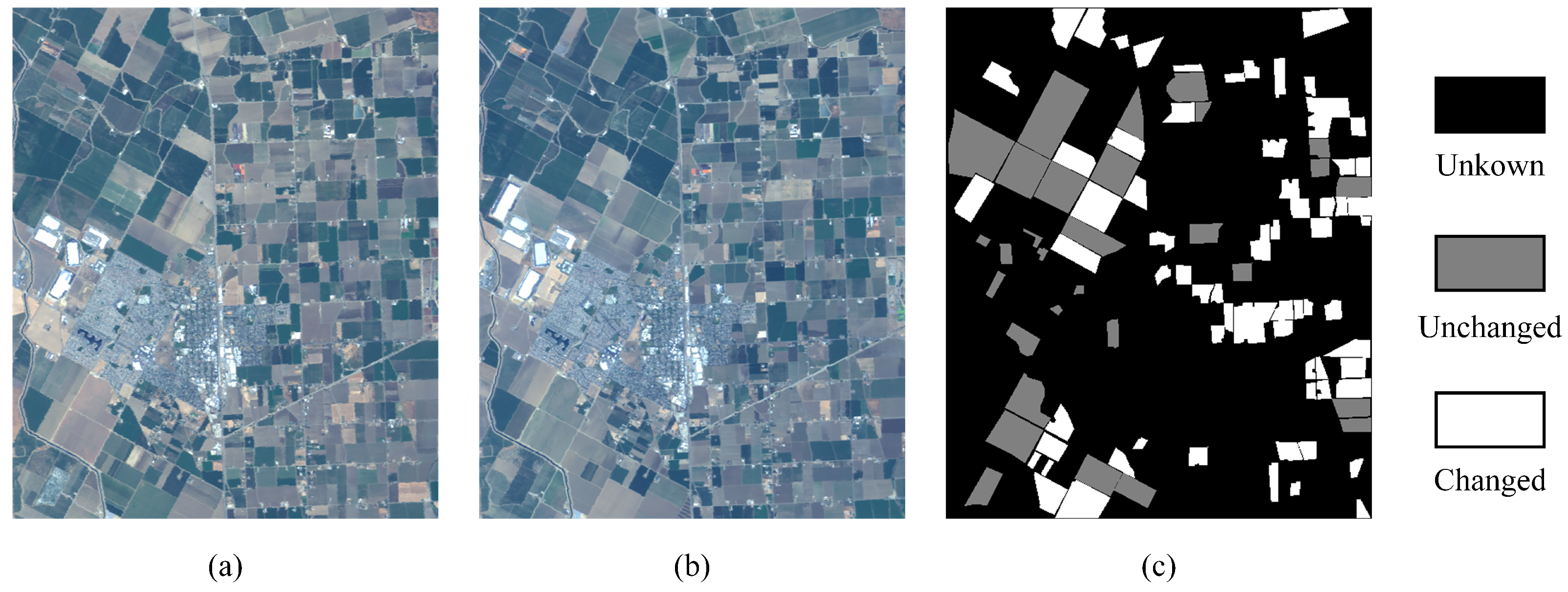
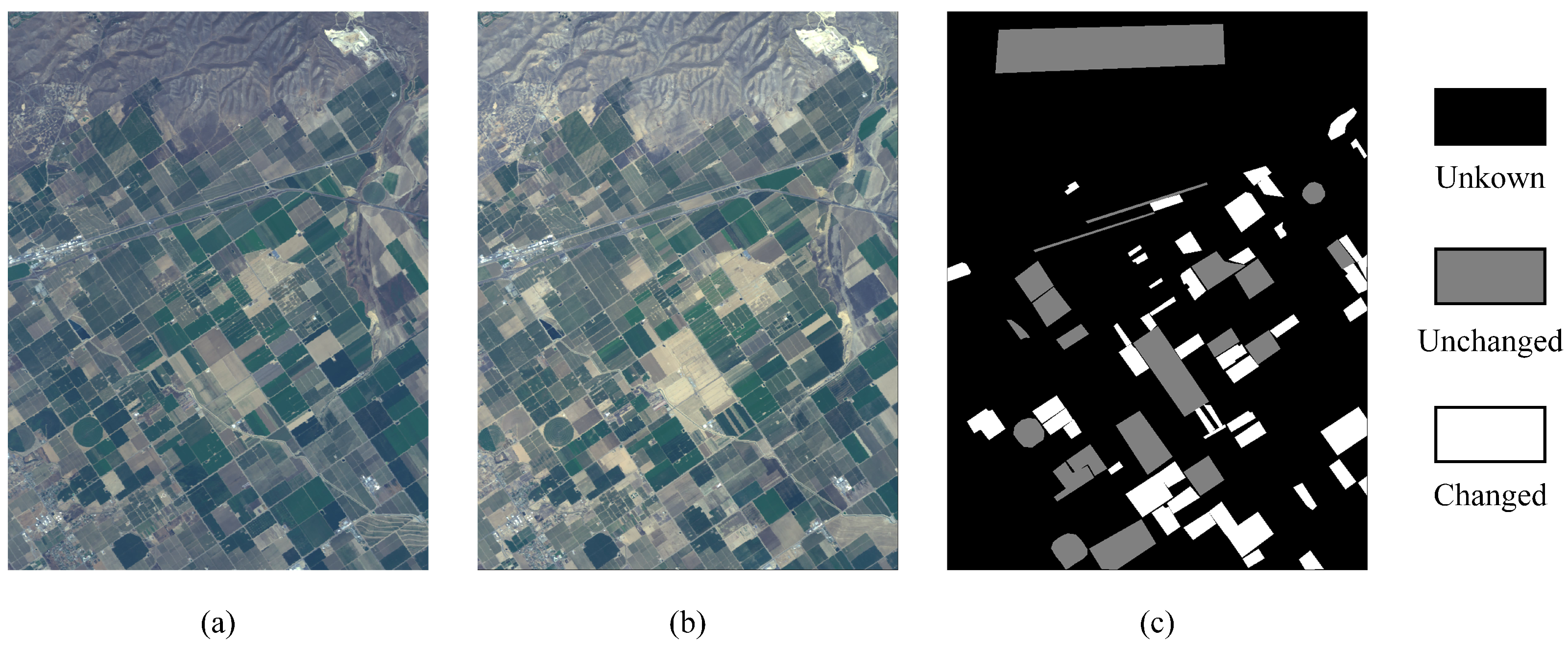
4.1. Datasets and Evaluation Criteria
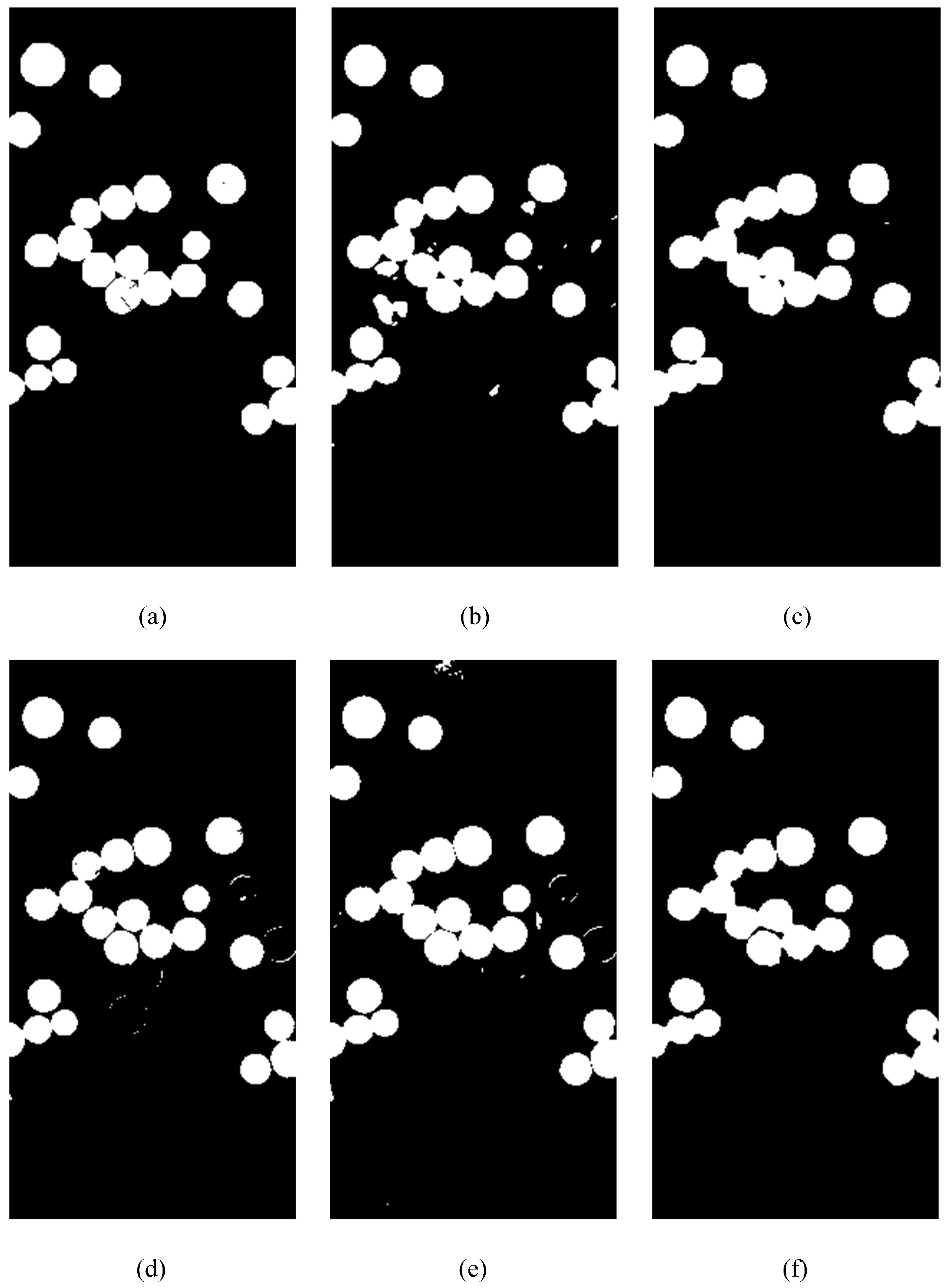
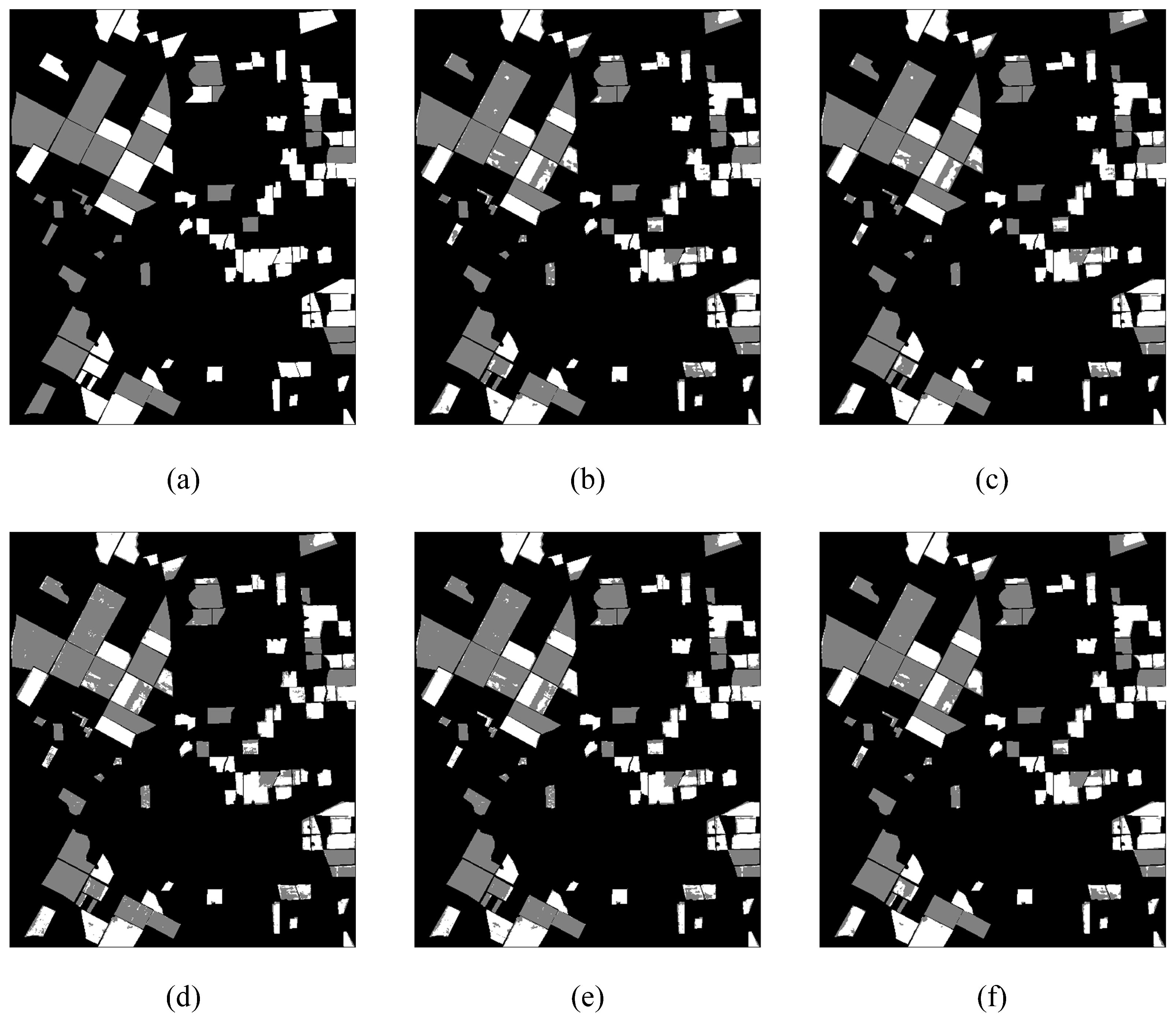
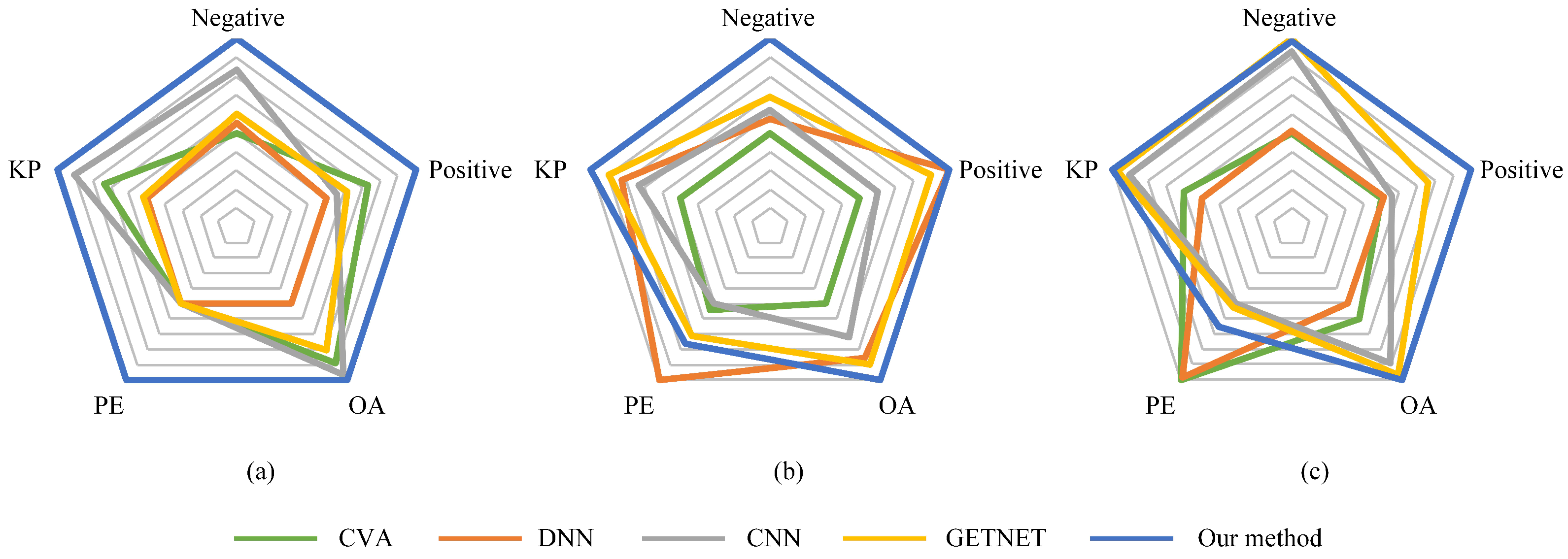
4.2. Comparison Results and Analysis
4.3. Ablation Study
5. Discussion
5.1. Effectiveness of RNN on Spectra
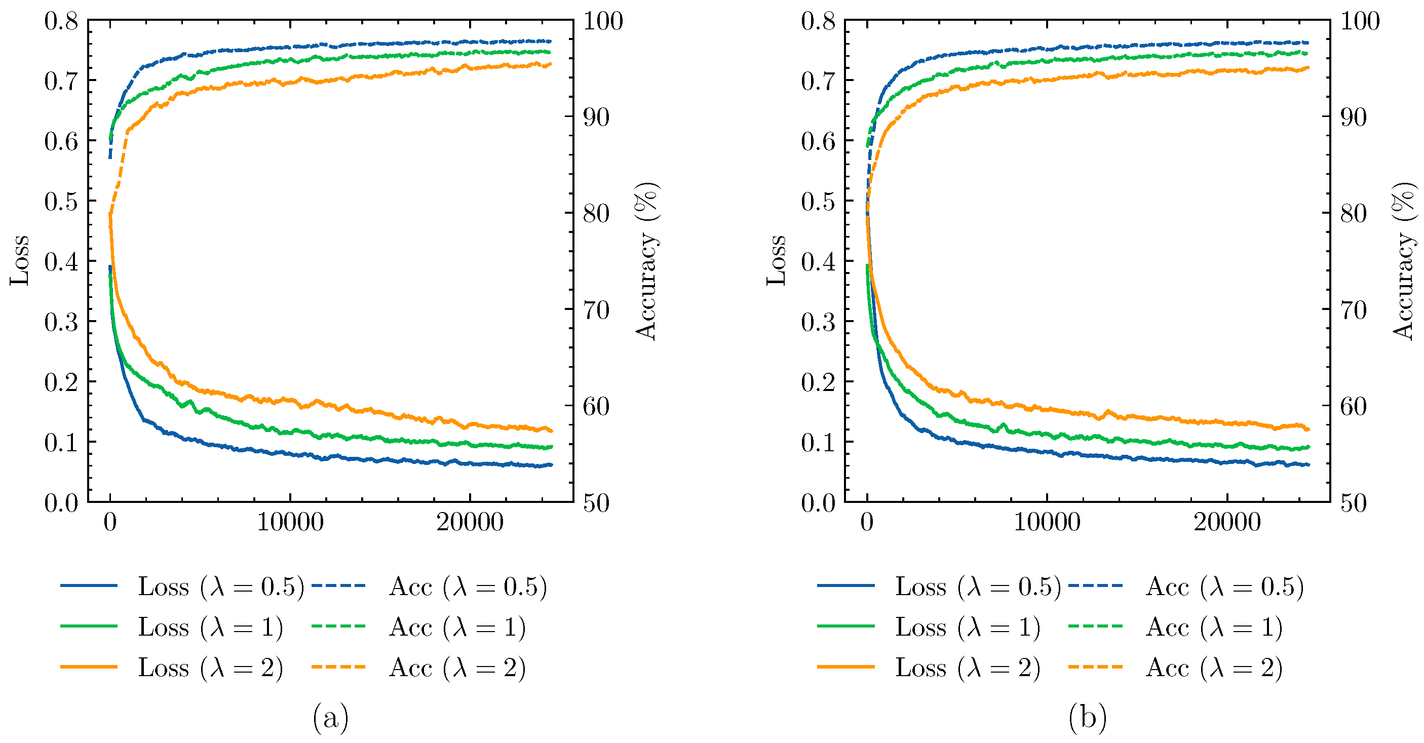
5.2. Selection of Hyperparameters in Sample Generation
5.3. Compare the Performance of the Algorithm
5.4. Shortcomings of This Paper and Future Work
6. Conclusions
Author Contributions
Funding
Conflicts of Interest
References
- Cheng, G.; Yao, Y.; Li, S.; Li, K.; Xie, X.; Wang, J.; Yao, X.; Han, J. Dual-aligned oriented detector. IEEE Trans. Geosci. Remote Sens. 2022, 60, 5618111. [Google Scholar] [CrossRef]
- Liu, J.; Gong, M.; Qin, K.; Zhang, P. A deep convolutional coupling network for change detection based on heterogeneous optical and radar images. IEEE Trans. Neural Netw. Learn. Syst. 2016, 29, 545–559. [Google Scholar] [CrossRef]
- Zhang, P.; Gong, M.; Su, L.; Liu, J.; Li, Z. Change detection based on deep feature representation and mapping transformation for multi-spatial-resolution remote sensing images. ISPRS J. Photogramm. Remote Sens. 2016, 116, 24–41. [Google Scholar] [CrossRef]
- Gong, M.; Zhan, T.; Zhang, P.; Miao, Q. Superpixel-based difference representation learning for change detection in multispectral remote sensing images. IEEE Trans. Geosci. Remote Sens. 2017, 55, 2658–2673. [Google Scholar] [CrossRef]
- Zhang, H.; Gong, M.; Zhang, P.; Su, L.; Shi, J. Feature-level change detection using deep representation and feature change analysis for multispectral imagery. IEEE Geosci. Remote Sens. Lett. 2016, 13, 1666–1670. [Google Scholar] [CrossRef]
- Wu, Y.; Mu, G.; Qin, C.; Miao, Q.; Ma, W.; Zhang, X. Semi-supervised hyperspectral image classification via spatial-regulated self-training. Remote Sens. 2020, 12, 159. [Google Scholar] [CrossRef]
- Wu, Y.; Li, J.; Yuan, Y.; Qin, A.K.; Miao, Q.; Gong, M. Commonality autoencoder: Learning common features for change detection from heterogeneous images. IEEE Trans. Neural Netw. Learn. Syst. 2021, 33, 4257–4270. [Google Scholar] [CrossRef]
- Cheng, G.; Wang, G.; Han, J. ISNet: Towards Improving Separability for Remote Sensing Image Change Detection. IEEE Trans. Geosci. Remote Sens. 2022, 60, 5623811. [Google Scholar] [CrossRef]
- Liu, J.; Gong, M.; Miao, Q.; Su, L.; Li, H. Change detection in synthetic aperture radar images based on unsupervised artificial immune systems. Appl. Soft Comput. 2015, 34, 151–163. [Google Scholar] [CrossRef]
- Zhao, Q.; Ma, J.; Gong, M.; Li, H.; Zhan, T. Three-class change detection in synthetic aperture radar images based on deep belief network. J. Comput. Theor. Nanosci. 2016, 13, 3757–3762. [Google Scholar] [CrossRef]
- Ma, W.; Wu, Y.; Gong, M.; Xiong, Y.; Yang, H.; Hu, T. Change detection in SAR images based on matrix factorisation and a Bayes classifier. Int. J. Remote Sens. 2019, 40, 1066–1091. [Google Scholar] [CrossRef]
- Wang, Q.; Yuan, Z.; Du, Q.; Li, X. GETNET: A general end-to-end 2-D CNN framework for hyperspectral image change detection. IEEE Trans. Geosci. Remote Sens. 2018, 57, 3–13. [Google Scholar] [CrossRef]
- Deng, J.; Wang, K.; Deng, Y.; Qi, G. PCA-based land-use change detection and analysis using multitemporal and multisensor satellite data. Int. J. Remote Sens. 2008, 29, 4823–4838. [Google Scholar] [CrossRef]
- Bovolo, F.; Marchesi, S.; Bruzzone, L. A framework for automatic and unsupervised detection of multiple changes in multitemporal images. IEEE Trans. Geosci. Remote Sens. 2011, 50, 2196–2212. [Google Scholar] [CrossRef]
- Liu, S.; Bruzzone, L.; Bovolo, F.; Zanetti, M.; Du, P. Sequential spectral change vector analysis for iteratively discovering and detecting multiple changes in hyperspectral images. IEEE Trans. Geosci. Remote Sens. 2015, 53, 4363–4378. [Google Scholar] [CrossRef]
- Thonfeld, F.; Feilhauer, H.; Braun, M.; Menz, G. Robust Change Vector Analysis (RCVA) for multi-sensor very high resolution optical satellite data. Int. J. Appl. Earth Obs. Geoinf. 2016, 50, 131–140. [Google Scholar] [CrossRef]
- Malila, W. Change vector analysis: An approach for detecting forest changes with Landsat. In Proceedings of the Machine Processing of Remotely Sensed Data Symposium, Purdue University, West Lafayette, IN, USA, 3–6 June 1980; pp. 326–335. [Google Scholar]
- Bruzzone, L.; Prieto, D.F. Automatic analysis of the difference image for unsupervised change detection. IEEE Trans. Geosci. Remote Sens. 2000, 38, 1171–1182. [Google Scholar] [CrossRef]
- Bovolo, F.; Bruzzone, L. A theoretical framework for unsupervised change detection based on change vector analysis in the polar domain. IEEE Trans. Geosci. Remote Sens. 2006, 45, 218–236. [Google Scholar] [CrossRef]
- Saha, S.; Bovolo, F.; Bruzzone, L. Unsupervised deep change vector analysis for multiple-change detection in VHR images. IEEE Trans. Geosci. Remote Sens. 2019, 57, 3677–3693. [Google Scholar] [CrossRef]
- Nielsen, A.A.; Conradsen, K.; Simpson, J.J. Multivariate alteration detection (MAD) and MAF postprocessing in multispectral, bitemporal image data: New approaches to change detection studies. Remote Sens. Environ. 1998, 64, 1–19. [Google Scholar] [CrossRef]
- Gong, M.; Zhou, Z.; Ma, J. Change detection in synthetic aperture radar images based on image fusion and fuzzy clustering. IEEE Trans. Image Process. 2011, 21, 2141–2151. [Google Scholar] [CrossRef] [PubMed]
- Celik, T. Unsupervised change detection in satellite images using principal component analysis and k-means clustering. IEEE Geosci. Remote Sens. Lett. 2009, 6, 772–776. [Google Scholar] [CrossRef]
- Nielsen, A.A. The regularized iteratively reweighted MAD method for change detection in multi-and hyperspectral data. IEEE Trans. Image Process. 2007, 16, 463–478. [Google Scholar] [CrossRef] [PubMed]
- Tang, P.; Yang, J.; Zhang, C.; Zhu, D.; Su, W. An object-oriented post-classification remote sensing change detection after the pixel ratio. Remote Sens. Inf. 2010, 1, 69–72. [Google Scholar]
- Al Rawashdeh, S.B. Evaluation of the differencing pixel-by-pixel change detection method in mapping irrigated areas in dry zones. Int. J. Remote Sens. 2011, 32, 2173–2184. [Google Scholar] [CrossRef]
- Liu, S.; Bruzzone, L.; Bovolo, F.; Du, P. Unsupervised multitemporal spectral unmixing for detecting multiple changes in hyperspectral images. IEEE Trans. Geosci. Remote Sens. 2016, 54, 2733–2748. [Google Scholar] [CrossRef]
- Hsieh, C.C.; Hsieh, P.F.; Lin, C.W. Subpixel change detection based on abundance and slope features. In Proceedings of the 2006 IEEE International Symposium on Geoscience and Remote Sensing, Denver, CO, USA, 31 July–4 August 2006; pp. 775–778. [Google Scholar]
- Ertürk, A.; Iordache, M.D.; Plaza, A. Sparse unmixing with dictionary pruning for hyperspectral change detection. IEEE J. Sel. Top. Appl. Earth Obs. Remote Sens. 2016, 10, 321–330. [Google Scholar] [CrossRef]
- Ertürk, A.; Iordache, M.D.; Plaza, A. Sparse unmixing-based change detection for multitemporal hyperspectral images. IEEE J. Sel. Top. Appl. Earth Obs. Remote Sens. 2015, 9, 708–719. [Google Scholar] [CrossRef]
- Li, H.; Wu, K.; Xu, Y. An Integrated Change Detection Method Based on Spectral Unmixing and the CNN for Hyperspectral Imagery. Remote Sens. 2022, 14, 2523. [Google Scholar] [CrossRef]
- Qu, Y.; Wang, W.; Guo, R.; Ayhan, B.; Kwan, C.; Vance, S.; Qi, H. Hyperspectral anomaly detection through spectral unmixing and dictionary-based low-rank decomposition. IEEE Trans. Geosci. Remote Sens. 2018, 56, 4391–4405. [Google Scholar] [CrossRef]
- Seydi, S.T.; Hasanlou, M. A new structure for binary and multiple hyperspectral change detection based on spectral unmixing and convolutional neural network. Measurement 2021, 186, 110137. [Google Scholar] [CrossRef]
- Seydi, S.T.; Shah-Hosseini, R.; Hasanlou, M. New framework for hyperspectral change detection based on multi-level spectral unmixing. Appl. Geomat. 2021, 13, 763–780. [Google Scholar] [CrossRef]
- Huang, F.; Yu, Y.; Feng, T. Hyperspectral remote sensing image change detection based on tensor and deep learning. J. Vis. Commun. Image Represent. 2019, 58, 233–244. [Google Scholar] [CrossRef]
- Zhan, Y.; Fu, K.; Yan, M.; Sun, X.; Wang, H.; Qiu, X. Change detection based on deep siamese convolutional network for optical aerial images. IEEE Geosci. Remote Sens. Lett. 2017, 14, 1845–1849. [Google Scholar] [CrossRef]
- Mou, L.; Bruzzone, L.; Zhu, X.X. Learning spectral-spatial-temporal features via a recurrent convolutional neural network for change detection in multispectral imagery. IEEE Trans. Geosci. Remote Sens. 2018, 57, 924–935. [Google Scholar] [CrossRef]
- Ken, S.; Akayuki, O. Change Detection from a Street Image Pair Using CNN Features and Superpixel Segmentation. 2015. Available online: http://www.ucl.nuee.nagoya-u.ac.jp/~sakurada/document/71-Sakurada-BMVC15.pdf (accessed on 1 September 2022).
- Wang, Q.; Zhang, X.; Chen, G.; Dai, F.; Gong, Y.; Zhu, K. Change detection based on Faster R-CNN for high-resolution remote sensing images. Remote Sens. Lett. 2018, 9, 923–932. [Google Scholar] [CrossRef]
- Li, X.; Yuan, Z.; Wang, Q. Unsupervised deep noise modeling for hyperspectral image change detection. Remote Sens. 2019, 11, 258. [Google Scholar] [CrossRef]
- Li, L.; Yang, Z.; Jiao, L.; Liu, F.; Liu, X. High-resolution SAR change detection based on ROI and SPP net. IEEE Access 2019, 7, 177009–177022. [Google Scholar] [CrossRef]
- Gao, F.; Wang, X.; Gao, Y.; Dong, J.; Wang, S. Sea ice change detection in SAR images based on convolutional-wavelet neural networks. IEEE Geosci. Remote Sens. Lett. 2019, 16, 1240–1244. [Google Scholar] [CrossRef]
- Zhang, X.; Su, H.; Zhang, C.; Atkinson, P.M.; Tan, X.; Zeng, X.; Jian, X. A Robust Imbalanced SAR Image Change Detection Approach Based on Deep Difference Image and PCANet. arXiv 2020, arXiv:2003.01768. [Google Scholar]
- Liu, J.; Chen, K.; Xu, G.; Sun, X.; Yan, M.; Diao, W.; Han, H. Convolutional neural network-based transfer learning for optical aerial images change detection. IEEE Geosci. Remote Sens. Lett. 2019, 17, 127–131. [Google Scholar] [CrossRef]
- Zhou, Y.; Li, X. Unsupervised Self-training Algorithm Based on Deep Learning for Optical Aerial Images Change Detection. arXiv 2020, arXiv:2010.07469. [Google Scholar]
- López-Fandiño, J.; Garea, A.S.; Heras, D.B.; Argüello, F. Stacked autoencoders for multiclass change detection in hyperspectral images. In Proceedings of the IGARSS 2018—2018 IEEE International Geoscience and Remote Sensing Symposium, Valencia, Spain, 22–27 July 2018; pp. 1906–1909. [Google Scholar]


| Stage | Module | Parameter |
|---|---|---|
| Block1 | Conv | channel = 128 |
| size = 1 | ||
| ReLU | ||
| Conv | channel = 128 | |
| stride = 2 | ||
| size = 3 | ||
| ReLU | ||
| Block2 | RNN | channel = 32 |
| Tanh | ||
| Conv | channel = 32 | |
| stride = 2 | ||
| size = 3 | ||
| ReLU | ||
| Block3 | RNN | channel = 8 |
| Tanh | ||
| Conv | channel = 8 | |
| stride = 2 | ||
| size = 3 | ||
| ReLU | ||
| Flatten | ||
| Head | Linear | channel = 32 |
| ReLU | ||
| Linear | channel = 8 | |
| ReLU | ||
| Linear | channel = 2 |
| Algorithm | Negative | Positive | OA | PE | KC |
|---|---|---|---|---|---|
| CVA | 0.99 | 0.90 | 97.94 | 77.30 | 90.93 |
| DNN | 0.99 | 0.96 | 98.40 | 78.20 | 92.68 |
| CNN | 0.99 | 0.91 | 98.22 | 77.22 | 92.20 |
| GETNET | 0.99 | 0.94 | 98.45 | 77.63 | 93.08 |
| Ours (without RNN) | 0.99 | 0.94 | 98.37 | 77.66 | 92.70 |
| Ours (with RNN) | 0.99 | 0.95 | 98.58 | 77.73 | 93.63 |
| Algorithm | Negative | Positive | OA | PE | KC |
|---|---|---|---|---|---|
| CVA | 0.78 | 0.95 | 85.37 | 49.55 | 71.00 |
| DNN | 0.78 | 0.94 | 82.73 | 49.54 | 69.73 |
| CNN | 0.79 | 0.94 | 85.84 | 49.60 | 71.91 |
| GETNET | 0.78 | 0.94 | 84.80 | 49.57 | 69.85 |
| Ours | 0.79 | 0.95 | 86.08 | 59.55 | 72.41 |
| Algorithm | Negative | Positive | OA | PE | KC |
|---|---|---|---|---|---|
| CVA | 0.88 | 0.79 | 84.74 | 51.96 | 68.23 |
| DNN | 0.88 | 0.79 | 84.06 | 51.94 | 66.83 |
| CNN | 0.92 | 0.79 | 86.59 | 51.28 | 72.47 |
| GETNET | 0.93 | 0.80 | 87.03 | 51.24 | 73.39 |
| Ours | 0.92 | 0.81 | 87.25 | 51.46 | 73.72 |
| Network Structure | Parameters | FLOPs |
|---|---|---|
| Without RNN | 0.221M | 43.679M |
| With RNN | 0.192M | 42.277M |
| Method | Pearson Correlation Coefficients |
|---|---|
| CNN-based | −0.398 |
| RNN-based | 0.275 |
Publisher’s Note: MDPI stays neutral with regard to jurisdictional claims in published maps and institutional affiliations. |
© 2022 by the authors. Licensee MDPI, Basel, Switzerland. This article is an open access article distributed under the terms and conditions of the Creative Commons Attribution (CC BY) license (https://creativecommons.org/licenses/by/4.0/).
Share and Cite
Zhao, H.; Feng, K.; Wu, Y.; Gong, M. An Efficient Feature Extraction Network for Unsupervised Hyperspectral Change Detection. Remote Sens. 2022, 14, 4646. https://doi.org/10.3390/rs14184646
Zhao H, Feng K, Wu Y, Gong M. An Efficient Feature Extraction Network for Unsupervised Hyperspectral Change Detection. Remote Sensing. 2022; 14(18):4646. https://doi.org/10.3390/rs14184646
Chicago/Turabian StyleZhao, Hongyu, Kaiyuan Feng, Yue Wu, and Maoguo Gong. 2022. "An Efficient Feature Extraction Network for Unsupervised Hyperspectral Change Detection" Remote Sensing 14, no. 18: 4646. https://doi.org/10.3390/rs14184646
APA StyleZhao, H., Feng, K., Wu, Y., & Gong, M. (2022). An Efficient Feature Extraction Network for Unsupervised Hyperspectral Change Detection. Remote Sensing, 14(18), 4646. https://doi.org/10.3390/rs14184646