Estimating Crop Seed Composition Using Machine Learning from Multisensory UAV Data

Abstract

The pre-harvest estimation of seed composition from standing crops is imperative for field management practices and plant phenotyping. This paper presents for the first time the potential of Unmanned Aerial Vehicles (UAV)-based high-resolution hyperspectral and LiDAR data acquired from in-season stand crops for estimating seed protein and oil compositions of soybean and corn using multisensory data fusion and automated machine learning. UAV-based hyperspectral and LiDAR data was collected during the growing season (reproductive stage five (R5)) of 2020 over a soybean test site near Columbia, Missouri and a cornfield at Urbana, Illinois, USA. Canopy spectral and texture features were extracted from hyperspectral imagery, and canopy structure features were derived from LiDAR point clouds. The extracted features were then used as input variables for automated machine-learning methods available with the H2O Automated Machine-Learning framework (H2O-AutoML). The results presented that: (1) UAV hyperspectral imagery can successfully predict both the protein and oil of soybean and corn with moderate accuracies; (2) canopy structure features derived from LiDAR point clouds yielded slightly poorer estimates of crop-seed composition compared to the hyperspectral data; (3) regardless of machine-learning methods, the combination of hyperspectral and LiDAR data outperformed the predictions using a single sensor alone, with an R² of 0.79 and 0.67 for corn protein and oil and R² of 0.64 and 0.56 for soybean protein and oil; and (4) the H2O-AutoML framework was found to be an efficient strategy for machine-learning-based data-driven model building. Among the specific regression methods evaluated in this study, the Gradient Boosting Machine (GBM) and Deep Neural Network (NN) exhibited superior performance to other methods. This study reveals opportunities and limitations for multisensory UAV data fusion and automated machine learning in estimating crop-seed composition.

1. Introduction

The global population is estimated to increase almost 40% from 7.8 billion to 9.6 billion by 2050 [1], requiring a 70% increase in global food production [2]. Food security is increasingly becoming a critical issue around the globe due to climate change and population growth [3,4]. As staple crops, soybean (Glycine max L. Merrill) and corn (Zea mays L.) are used for multiple purposes, such as food for humans, feed for livestock and ingredients for a green alternative energy resource biodiesel [5]. The composition of soybean and corn make them reliable primary feedstocks for bioenergy production. About 50% of biodiesel feedstock in the United States comes from soybean oil [6], and 94% of ethanol production comes from corn starch [7].

Due to their nutritional and economic values, improving their productivity and quality is significant for farmers and companies seeking higher yield and profitability [8]. Seed composition primarily refers to major constituents found within the seed, including the protein, oil, fatty acids and carbohydrates, and it also extends to other less-prominent components, such as isoflavones and minerals, which determine the seed’s nutritional value [9].

A good understanding of seed composition and the factors that modulate it is critical to improving its quality through management practices and breeding efforts to achieve composition targets [10]. A variety of approaches have been developed and implemented to assess seed composition. Wet-chemistry laboratory analysis is a traditional standard method for seed-composition measurement, which is accurate but expensive and time-consuming.

In recent years, non-destructive and less expensive lab-based methods have also been widely employed to determine seed composition in agriculture and food industries. These non-destructive lab-based methods often leverage spectral or other signals retrieved from crop seed to predict chemical component composition. Specifically, techniques, such as Near-infrared (NIR) spectroscopy, Middle infrared spectroscopy (MIR) [11,12], Raman spectroscopy [13], as well as Nuclear Magnetic Resonance Spectrometry (NMRS) [14] have been used to assess both major seed components, such as the protein, oil and fatty acids, and micronutrients composition, such as B, Ca, Cu, Fe, Mg, Mn, Mo and Zn [11,12].

Lab-based methods, either destructive or non-destructive, take measurements directly from seeds; additionally, those methods are only applicable after harvest when the seeds are available and cannot be used to predict seed composition while the crops are in the field. Field-based methods use ground or aerial platforms and sensors to acquire data from standing crops during the growing season and offer opportunities to estimate seed composition before the harvest.

Canopy spectral signals obtained from ground-based handheld spectroscopy have been used for seed composition estimation for a variety of crops, including rice [15], wheat [16,17], barley [18,19] and soybean [20,21]. Airborne platform-based hyperspectral remote sensing has also been used for predicting wheat grain protein content [22] and soybean protein and oil composition [23]. Additionally, satellite remote sensing showed its potential for grain chemical component estimation, such as wheat protein, at a large scale using multispectral imagery [24,25,26].

In recent years, Unmanned Aerial Vehicles (UAV) have been employed in various agricultural applications. The flexibility, low cost and the ability to collect data at high spatial, spectral and temporal resolution, have contributed to the popularity of UAV for diverse applications, including precision agriculture and plant phenotyping [27,28]. While monitoring and assessment of crop growth, health and stress status have dominated the applications for UAV in agriculture, UAV have also been used for seed protein composition estimation in rice [29,30] and wheat [31] using multispectral imaging.

Notably, the versatility of the UAV platforms enables the integration of multiple sensors, providing opportunities for implementing multisensory data fusion. The combination of data acquired from different sensors mounted on UAV becomes popular because an amalgamation of thermal, spatial, structural and spectral information from various sensors provides complementary canopy information, thus, increasing the accuracy of assessing plant traits [28,32,33].

Previous studies on estimating seed composition using remote sensing mainly leveraged canopy spectral features, such as reflectance bands or vegetation indices (VIs), as input variables for prediction model development [21,23,31]. Texture features of remote sensing imagery consider both spectral and spatial domains and suppress the noise that often happens to spectral features, potentially offering additional information associated with canopy spatial and subtle structure characteristics [34]. Texture features can provide comparable or even superior performance for the estimation of various plant traits and grain yield [35,36].

Nonetheless, the potential of texture features has not been investigated in estimating crop-seed composition. It is worth noting that remote-sensing-imagery-based canopy spectral information often undergoes optical saturation issues when the plant canopy has higher Leaf Area Index (LAI) (i.e., >3.0) [35,37,38,39]; furthermore, remote-sensing-imagery-based spectral information only captures a top-view of the canopy growth status and misses data of three-dimensional (3D) canopy vertical profile (the canopy height, canopy structure, etc.); this potentially further limits its applications in spatially heterogeneous and dense agricultural fields [28,40].

Canopy structure features that contain 3D canopy information have been derived from photogrammetry or LiDAR-based point clouds and have been successfully implemented in estimating a variety of plant traits, such as biomass and LAI estimation [41,42] and crop yield prediction [35,43]. However, point-cloud-based canopy structure information has not been used for crop-seed-composition estimation. The formation of seed composition depends on multiple factors, including biotic and abiotic conditions, such as sunshine hours and water and nutrient availability.

Sunlight is the most crucial element that catalyzes photosynthetic activity, and the canopy architecture (the closure, canopy height and leaf angle distribution, etc.) plays a vital role in light absorption by plants [44]. Although LiDAR point-cloud-based canopy structure information does not directly relate to photosynthetic activities, it characterizes canopy structure patterns, such as canopy closure status, canopy height and leaf angle distribution, thus, affecting the seed composition [45]. Therefore, with respect to agronomic mechanisms, canopy structure information could potentially be applied in estimating the crop-seed composition.

Moreover, due to the weakened optical saturation issues, along with complementary information, a combination of canopy spectral information (i.e., VIs) obtained from multispectral/hyperspectral imagery with point-cloud-based 3D canopy structure features has proved to yield more robust models with improved accuracies in plant traits estimation and grain yield prediction in many cases [28,43,46,47]. Nonetheless, multisensory data fusion/combination (in particular, the combination of UAV hyperspectral and LiDAR data-derived canopy spectral and structure features) has not been examined in estimating crop-seed composition.

Rapid advances in machine learning (ML) provide enormous opportunities to develop remote sensing-based data-driven models for crop monitoring, plant trait estimations and grain yield prediction [48,49,50,51]. ML conducts the efficient identification of complex-linear/non-linear relationships, and extracting spatiotemporal features automatically from various input variables has the potential to better estimate plant traits and grain yield and potentially seed composition [52].

The recent development of automated machine learning frameworks, such as H2O Automated Machine Learning (H2O-AutoML) [53] and AutoKeras [54], facilitates the implementation of ML in remote sensing-based applications through automated and streamlined feature selection, hyperparameter optimization and model evaluation functions [52,55]. However, automated ML frameworks have not been broadly employed in remote-sensing agricultural applications; in particular, it has not been attempted in crop-seed-composition estimation.

Therefore, this research aims to: (1) evaluate the potential of UAV-based hyperspectral and LiDAR data, as well as their combination for the estimation of seed protein and oil composition of soybean and corn; and (2) to evaluate the potential of machine-learning methods, particularly the automated machine learning framework H2O-AutoML in crop-seed-composition estimation.

2. Test Site and Data

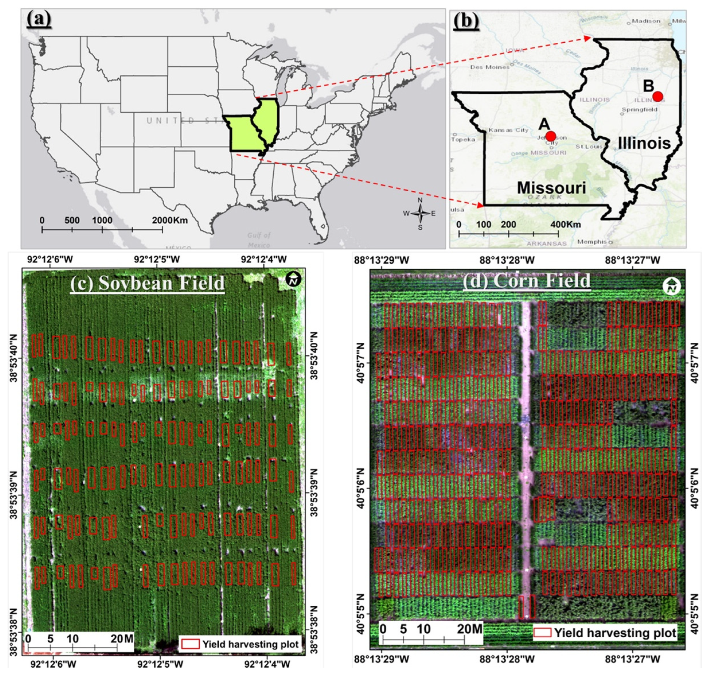
2.1. Test Sites

2.1.1. Soybean Field and Experiment Setup

A soybean experiment was conducted at the University of Missouri’s Bradford Research Center (BRC) near Columbia, Missouri, USA (Figure 1). The field is 77 m in length and 65 m in width. The field used for this experiment was modified to restrict the maximum rooting depth, and roots can explore to 0.3, 0.45, 0.6, 0.75 or 0.9 m depth [56]. These rooting restriction treatments were established more than 40 years ago by inserting a plastic liner at the respective depths in excavated channels separated by undisturbed buffer areas. After adding drainage tiles on top of the plastic liner to avoid waterlogging, the channels were refilled with soil. Restricting the rooting zone to different depths generates treatments that also differ in the amount of plant-available soil moisture.

A maturity group 4.4 (‘Pioneer P44A37L’) and a maturity group 2.9 (‘Pioneer P29A85L’) soybean cultivars were no-till sown in strips perpendicular to the five different rooting depth zones in two different row-spacing (0.38 and 0.76 m) on 8 June 2020. Both row-spacing treatments were sown to a density of 347,000 seeds per hectare. Cultivars and row spacings were randomly arranged within four replications. The two cultivars, five rooting depth treatments and two-row spacings resulted in 20 different treatments.

Weeds were controlled using a burn-down treatment and pre-emergence herbicide application. Post-emergence weed control was conducted by glufosinate and complemented with manual mechanical removal. According to the onsite Bradford weather station, the study area has a humid continental climate. The average monthly growing season temperatures reach 24.8 °C in July and go down to 10.7 °C in October. Average monthly perceptions were 89 mm in May, 156 mm in June, 94 mm in July, 113 mm in August, 96 mm in September and 35 mm in October.

2.1.2. Cornfield and Experiment Setup

The experimental cornfield is located in Urbana, Illinois, at the Crop Sciences Research and Education Center near the campus of the University of Illinois at Urbana-Champaign (Figure 1). The field is 100 m in length and 82 m in width. Sixty-two corn hybrids were planted on 12 May 2020 in a split-plot design where each genotype was paired in adjacent plots receiving either no supplemental N fertilizer or granular ammonium sulfate applied to a band near the plants at a rate of 225 kg N per hectare.

N was applied on 3 June 2020, when plants were at the V3 growth stage. Each plot was 5.3 m long and 0.76 m wide. The field was rainfed and received no supplemental irrigation. Plots were maintained weed-free by pre-plant and post-emergence (15 June) applications of herbicide (atrazine + metolachlor + mesotrione), followed by hand cultivation as needed.

The nearby weather station shows that the average monthly temperatures were 25.1 °C in July and dropped to 11.4 °C in October. The average monthly perceptions were 104 mm in May, 149 mm in June, 120 mm in July, 34 mm in August, 74 mm in September and 66 mm in October.

2.2. Data Acquisition

2.2.1. Soybean Grain Yield Sampling and Seed Composition Measurement

Soybean harvest was conducted on 20 November 2020, using a small-plot research combine. A total of 91 plots (the locations of those plots are marked with red polygons in the “(A) Soybean Field” image in Figure 1) across the soybean field were selected and used for yield harvesting. An area measuring 4.57 m in length and 1.52 m in width was harvested from the center of each plot to determine the grain yield. A subsample of 60 mL of harvested soybean seeds per plot was used to measure the soybean seed composition (protein, oil, carbohydrates, fatty acids and amino acids) using a lab-based NIR spectrometer (Perkin Elmer, DA 7250 NIR Analyzer, Waltham, MA, USA).

2.2.2. Corn Grain Yield Sampling and Seed Composition Measurement

Corn harvesting was conducted on four different days in 2020 to ensure that each plot was harvested when the plants reached physiological maturity prior to full senescence (R6 growth stage). Five representative plants from each two-row plot were harvested manually by cutting the plant at the base of the stalk, removing the cob and grain and then drying the ears at 35 °C until reaching a target grain moisture of approximately 10%.

A total of 369 plots (locations of those plots were marked with the red polygons in the “(B) Corn Field” image in Figure 1) across the corn field were selected and used for yield harvesting. Grain was shelled from the five ears, and two subsamples of approximately 300 mL volume were measured for seed composition (protein, oil, starch and water) using a Perkin Elmer DA 7200 NIR Analyzer (Waltham, MA, USA) and a custom-built calibration that includes samples representing a broad range of maize grain compositions.

A summary of the statistics on lab-based seed protein and oil compositions from soybean and corn is displayed in

Table 1. Summary statistics of soybean and corn seed composition datasets.

Seed Composition	*NO.	Mean	Max.	Min.	SD	CV (%)
Soybean protein (%)	91	38.5	41.2	36.7	0.87	2.3%
Soybean oil (%)	91	22.9	24.5	21.0	0.83	3.6%
Corn protein (%)	369	7.7	15.3	5.7	1.45	18.9%
Corn oil (%)	369	3.9	5.3	2.1	0.57	14.5%

*NO.: Number of total yield samples; SD: standard deviation; CV: coefficient of variation.

. Additionally, the scatter plot of protein against oil and the distribution of protein and oil composition data are shown in Figure 2.

2.2.3. UAV Data Collection

Field campaigns were conducted to collect UAV hyperspectral and LiDAR data from the soybean field (Columbia, MO, USA) on 24 July 2020 (reproductive five stage of soybean) and the corn field (Champaign, IL, USA) on 26 August 2020 (reproductive five stage of corn). ). UAV hyperspectral and LiDAR systems described below were owned and operated by the Remote Sensing Lab at the Taylor Geospatial Institute. As shown in Figure 3 and

Table 2. Hyperspectral and LiDAR sensors used in this study.

Sensor	Vender/Brand	Recorded Info.	Spectral Properties	*GSD/ Point-Density
Hyperspectral	Headwall Hyperspec Nano	269 VNIR bands	400–1000 nm with FWHM of 6 nm	3 cm
LiDAR	Velodyne HDL-32	LAS point clouds	/	900 pts/m2

*GSD: ground sampling distances. Hyperspectral and LiDAR data were collected at 50 m; VNIR: visible and near-infrared; FWHM: full width at half maximum; and nm: nanometer.

, the Headwall Nano-Hyperspec sensor (Headwall Photonics Inc., Boston, MA, USA) mounted on a DJI M600 Pro UAV platform (DJI Technology Co., Ltd., Shenzhen, China) was used for hyperspectral data collection. The UAV platform has its GPS that mainly used for flight navigation.

Additionally, it is also equipped with an Applanix APX-15 GPS/inertial measuring unit (IMU) system (Applanix, Richmond Hill, ON, Canada) (Figure 3a). The hyperspectral sensor is fixed on a 3-axis gimbal system (Figure 3b), to cope with small fluctuations during the flight and acquire less distorted and high-quality image cube. The Headwall Nano-Hyperspec is a push broom scanner that collects data in the VNIR (visible and near-infrared) spectral range covering 400 to 1000 nm at 640 pixels spatial resolution and 12 bits radiometric resolution and generates hyperspectral image cubes with 269 spectral bands.

The UAV flight was conducted at 50 m height and 3 m/s speed, which generated imagery with 3 cm ground sampling distance (GSD) (Table 2). For radiometric calibration, a reflectance tarp that has three strips with distinct reflectance factors (56%, 30% and 11% reflectance) was set up in the field within the flight coverage during the flight (Figure 3c).

LiDAR data was acquired via the Phoenix Scout-32 system (Phoenix LiDAR Systems, Los Angeles, CA, USA) integrated on a DJI M600 Pro UAV platform (Figure 3d). The Phoenix Scout-32 system includes an RGB camera and a Velodyne HDL-32 LiDAR sensor (Figure 3e). The Velodyne HDL-32 LiDAR is a 32-channel dual-return sensor with a reported ±0.02 m accuracy (Table 2).

Additionally, an X900-GNSS (CHCNAV, Shanghai, China) ground-based RTK-GPS reference station (Figure 3f) was set up in the field during the LiDAR data collection to assist flight trajectory correction and generate point clouds with high accuracy [57]. The UAV flight mission for LiDAR data collection was planned using the Phoenix LiDAR Flight Planner tool (Phoenix LiDAR Systems, Los Angeles, CA, USA; www.phoenixlidar.com/flightplan, accessed on the dates of data collection in 2022), and the mission was conducted at a flight height of 50 m and a flight speed of 5 m/s.

2.2.4. UAV Data Preprocessing

Hyperspectral Image Processing

Radiometric calibration, geometric correction and orthomosaicing were applied to the raw hyperspectral image cubes via the SpectralView software (version 3.1.4) (Headwall Photonics, Fitchburg, MA, USA). Dark and white reference information taken before each flight along with the factory calibration files were used to convert the 12-bit digital numbers (D.N.s) of the raw data cubes to radiance values, and then the radiance values were further converted to surface reflectance factor by utilizing the imaged reflectance tarp [57].

Orthorectification and geometric correction were conducted by incorporating the 3D sensor positional information recorded by onboard IMU and high resolution (10 m) digital elevation model (DEM) through relevant functions of the SpectralView tool. Finally, the geometrically corrected and orthorectified reflectance image cubes were stitched as a single image cube covering the whole field [58]. Due to low flight height, the effect of the atmosphere was not considered in this work [59], and the atmospheric correction was not conducted. The mean and standard deviation (STD) of reflectance values of each band derived from sampling plots in soybean (Figure 4) and corn (Figure 4) fields are displayed below.

LiDAR Data Processing

To preprocess the LiDAR data, the cloud-based LiDAR data processing pipeline LiDARMill (Phoenix LiDAR Systems, Los Angeles, CA, USA), software version 3 was employed. Specifically, the raw LiDAR point clouds, along with trajectory files and the GNSS ground reference station-based GPS information, was provided to the LiDARMill framework. Point cloud data processing in LiDARMill pipeline conducts IMU and GNSS data combination to generate smooth and accurate trajectory (SBET) files.

The detect flight lines reduce the processing time by automatically detecting and omitting turns and calibration maneuvers to focus on the data-collecting flight lines LiDAR snap process, which optimizes alignment parameters and minimizes offsets from multiple flight lines comparing geometric observations made across overlapping flight lines [60].

Finally, the pipeline provides classified (ground/non-ground) point clouds with ±2 cm position accuracy according to the LiDAR sensor manufacturer’s report. The preprocessed LiDAR point clouds of soybean and corn fields are displayed in Figure 5; note that the height dimension values of the point clouds are the elevation values, not the canopy height values. The red color points are mostly the higher canopy areas, and the blue color points represent the ground points primarily.

3. Methodology

3.1. Feature Extraction

3.1.1. Hyperspectral-Imagery-Based Feature Extraction

Table 3. Descriptions of spectral and structure features used for model building.

Spectral Features	Formulation	Ref.
269 raw bands	The reflectance value of each band	/
Ratio vegetation index	RVI = R800/R680	[61]
Simple Ratio Index750	SR705 = R750/R705	[62]
Modified Red Edge Simple Ratio Index	mSR705 = (R750 − R705)/(R750 + R705 − 2R445)	[63]
Normalized Difference Vegetation Index750	ND705 = (R750 − R445)/(R705 − R445)	[63]
Modified Normalized Difference Vegetation Index	mND705 = (R750 − R445)/(R700 − R445)	[63]
Modified simple ratio	MSR = (R800/R700 − 1)/(R800/R700 + 1)0.5	[64]
Difference vegetation index	DVI = R800 − R680	[65]
Red-edge Chlorophyll Index	CIred-edge = R790/R720 − 1	[66]
Green Chlorophyll Index	CIgreen=(R840 − R870)/R550 − 1	[66]
Normalized difference vegetation index	NDVI = (R800 − R670)/(R800 + R670)	[61]
Green normalized difference vegetation index	GNDVI = (R750 – R550)/(R750 + R550)	[67]
Normalized difference red-edge	NDRE = (R790 − R720)/(R790 + R720)	[68]
MERIS terrestrial Chlorophyll index	MTCI = (R754 − R709)/(R709 − R681)	[69]
The enhanced vegetation index	EVI = 2.5((R800 − R670)/(R800+6R670 − 7.5R475 + 1))	[70]
Enhanced vegetation Index (2-band)	EVI2 = 2.5(R800 − R670)/(R800 + 2.4R670 + 1)	[71]
Improved soil adjusted vegetation index	MSAVI = 0.5[2R800 + 1 − ((2R800 + 1)0.5 − 8(R800 − R670))0.5]	[72]
Optimized soil adjusted vegetation index	OSAVI = 1.16(R800 − R670)/(R800 + R670 + 0.16)	[73]
Optimized soil adjusted vegetation index2	OSAVI2 = 1.16(R750 − R705)/(R750 + R705 + 0.16)	[74]
Modified chlorophyll absorption in reflectance index	MCARI = [(R700 − R670) − 0.2(R700 − R550)] (R700/R670)	[75]
Transformed chlorophyll absorption in reflectance index	TCARI = 3[(R700 − R670) − 0.2(R700 − R550) (R700/R670)]	[76]
MCARI/OSAVI	MCARI/OSAVI	[75]
TCARI/OSAVI	TCARI/OSAVI	[76]
Wide dynamic range vegetation index	WDRVI = (aR810 − R680)/(aR810 + R680) (a = 0.12)	[77]
Visible atmospherically resistance index	VARI = (R550 − R670)/(R550 + R670 − R475)	[78]
Triangular Vegetation Index	TVI = 0.5[120(R750 – R550) − 200(R670 – R550)]	[79]
Modified Triangular Vegetation Index 1	MTVI1 = 1.2[1.2(R800 – R550) − 2.5(R670 – R550)]	[80]
Modified Triangular Vegetation Index 2	MTVI2 = 1.5[1.2(R800 – R550) − 2.5(R670 – R550)]/[(2R800+1)2 − 6R800+5(R670)0.5 − 0.5)]0.5	[80]
Spectral Polygon Vegetation Index	SPVI = 0.4[3.7(R800 − R670) − 1.2|R530 − R670|]	[81]
Photochemical Reflectance Index	PRI = (R531 − R570)/(R531 + R570)	[82]
Renormalized difference vegetation index	RDVI = (R800 − R670)/(R800 + R670)0.5	[83]
Vogelmann Red Edge Index 1	VOG1 = R740/R720	[84]
Vogelmann Red Edge Index 2	VOG2 = (R734 − R747)/(R715 + R726)	[85]
Vogelmann Red Edge Index 3	VOG3 = (R734 − R747)/(R715 + R720)	[85]
Nonlinear Vegetation Index	NLI = (R8102 − R680)/(R8102 + R680)	[86]
Modified Nonlinear Vegetation Index	MNLI = (1 + 0.5) (R8102 − R680)/(R8102 + R680 + 0.5)	[87]

shows the spectral features derived from the UAV hyperspectral imagery. Specifically, for both soybean and cornfields, along with the original 269 reflectance bands of hyperspectral imagery, a set of vegetation indices that are commonly used for plant trait estimations and grain yield prediction were computed, and the plot-level mean values of each spectral feature were derived and used as input variables for the machine-learning-prediction models.

In addition to canopy spectral features, the grey level co-occurrence matrix (GLCM) canopy texture features were also derived from UAV hyperspectral imagery. GLCM, introduced by Haralick, et al. [88], is a widely used image texture feature in remote sensing applications. It characterizes the joint probability of pixel pairs at any grey level and statistically represents an image’s texture. To reduce the dimension and noise, the popular hyperspectral data denoising method Minimum Noise Fraction (MNF) [89] was applied to the hyperspectral data cube.

Based on the eigenvalue curve, the first 20 MNF components were selected for computing the GLCM. For each of these 20 layers, eight GLCM-based features—namely the mean (M.E.), variance (V.A.), homogeneity (H.O.), contrast (C.O.), dissimilarity (DI), entropy (EN), second moment (S.M.) and correlation (CC)—were calculated and used as hyperspectral sensor-based input variables for the machine-learning-prediction models (Figure 6). The details of the GLCM feature are presented in

Table 4. The grey level co-occurrence matrix (GLCM) texture features and their definitions.

NO.	Texture Measures	Formula
1	Mean (M.E.)	$ME={\displaystyle {\displaystyle \sum }_{k=0}^{N-1}}{\displaystyle {\displaystyle \sum }_{m=0}^{N-1}}k\times P\left(k,m\right)$
2	Variance (V.A.)	$VA={\displaystyle {\displaystyle \sum }_{k=0}^{N-1}}{\displaystyle {\displaystyle \sum }_{m=0}^{N-1}}{\left(k-\mu \right)}^{2}P\left(k,m\right)$
3	Homogeneity (H.O.)	$HO={\displaystyle {\displaystyle \sum }_{k=0}^{N-1}}{\displaystyle {\displaystyle \sum }_{m=0}^{N-1}}\frac{1}{1+{\left(k-m\right)}^2}P\left(k,m\right)$
4	Contrast (C.O.)	$CO={\displaystyle {\displaystyle \sum }_{i=0}^{N-1}}{\displaystyle {\displaystyle \sum }_{j=0}^{N-1}}P\left(i,j\right){\left(i-j\right)}^2$
5	Dissimilarity (DI)	$DI={\displaystyle {\displaystyle \sum }_{k=0}^{N-1}}{\displaystyle {\displaystyle \sum }_{m=0}^{N-1}}P\left(k,m\right)\left|k-m\right|$
6	Entropy (EN)	$EN=-{\displaystyle {\displaystyle \sum }_{k=0}^{N-1}}{\displaystyle {\displaystyle \sum }_{m=0}^{N-1}}P\left(k,m\right)\mathit{log}\left(P\left(k,m\right)\right)$
7	Second Moment (S.M.)	$SM={\displaystyle {\displaystyle \sum }_{k=0}^{N-1}}{\displaystyle {\displaystyle \sum }_{m=0}^{N-1}}{\left(P\left(k,m\right)\right)}^2$
8	Correlation (CC)	$CC={\displaystyle {\displaystyle \sum }_{k=0}^{N-1}}{\displaystyle {\displaystyle \sum }_{m=0}^{N-1}}P\left(k,m\right)\left[\frac{\left(k-ME\right)\left(m-ME\right)}{\sqrt{V{A}_{k}V{A}_m}}\right]$

Note: $P\left(i,j\right)=V\left(i,j\right)/{\displaystyle \sum }_{i=0}^{N-1}{\displaystyle \sum }_{j=0}^{N-1}V\left(i,j\right)$, where V(k,m) is the value in the cell k,m (row k and column m) of the moving window, and N is the number of rows or columns.

.

3.1.2. LiDAR Data-Based Canopy Structure Feature Extraction

A statistical outlier removal (SOR) algorithm was applied to remove outliers of the LiDAR point clouds [90]. Plot boundary polygons were used to split the point clouds of the whole field (Figure 5) and achieve plot-level point clouds, which resulted in a number of plot-level 3D point-cloud groups. For each point-cloud group, a Digital Terrain Model (DTM) was derived using the first percentile of the cumulative probability distribution of point clouds’ height values; thus, the actual height (or canopy height) for each point was derived by subtracting the DTM from original height value of each point of the Canopy Surface Model (CSM) [60].

Additionally, points below the first percentile of the cumulative probability distribution of original elevation were treated as ground points, while the remaining points were regarded as non-ground canopy points [91]. As shown in

Table 5. LiDAR point-cloud-derived canopy structure metrics.

Metrics	Descriptions
Hmax	Maximum of canopy height (intensity)
Hmin	Minimum of canopy height (intensity)
Hmean	Mean of canopy height (intensity)
Hmedian	Median of canopy height (intensity)
Hmode	Mode of canopy height (intensity)
Hsd	Standard deviation of canopy height (intensity)
Hcv	Coefficient of variation of canopy height (intensity)
Hmad	Hmad = 1.4826 × median (|height (intensity) − Hmedian (Imedian)|)
Haad	Haad = mean (|height (intensity) − Hmean (Imean)|)
Hper	Percentile of canopy height/intensity: H10 (I10), H20 (I20), H30 (I30), H40 (I40), H50 (I50), H60 (I60), H70 (I70), H80 (I80), H90 (I90), H95 (I95), H98 (I98), H99 (I99)
Hiqr	The Interquartile Range (iqr) of canopy height (intensity), Hiqr (Iiqr) = H75 (I75) − H25 (I25)
Hskn	Skewness of canopy height (intensity)
Hkurt	Kurtosis of canopy height (intensity)
Hcrd	Canopy return (intensity) density is the proportion of points (intensity) above the height quantiles (10th, 30th, 50th, 70th and 90th) to the total number of points (or sum of intensity): Hd10 (Id10), Hd30 (Id30), Hd50 (Id50), Hd70 (Id70) and Hd90 (Id90)
Hcrr	Canopy relief ratio of height (Intensity): (Hmean (Imean) − Hmin (Imin))/(Hmax (Imax) − Hmin (Imin))
Hlii	Laser intercept index (canopy returns/total returns), a description of fractional canopy cover.
Hcg	The ratio of canopy returns (intensity) and ground returns (intensity)

, a series of canopy height metrics that usually represent canopy structural characteristics were derived from each normalized plot-level point cloud. Additionally, LiDAR intensity-based metrics were extracted at plot level as well [60]. The point-cloud-based feature extraction procedure is presented in Figure 6.

3.2. Modeling Methods

3.2.1. Automated Machine Learning

The H2O-AutoML framework was employed in this work to build soybean and corn seed composition estimation models using UAV multisensory-derived canopy spectral, texture and structure features (Figure 6). H2O-AutoML supports supervised algorithms for classification and regression using tabular datasets. It conducts automated feature scaling, hyperparameter tuning and optimization through random grid searches and generates several models based on numerous model performance metrics.

Thus, this framework enables a time-efficient workflow to quickly find the optimal model without requiring manual trial and error. Additionally, H2O-AutoML also supports the efficient processing of large and complicated datasets. Major machine-learning algorithms available in H2O-AutoML are Gradient Boosting Machine (GBM), Generalized Linear Model (GLM), Distributed Random Forest (DRF),Extremely Randomized Trees (XRT) and Deep Neural Network (NN) [53,92].

Gradient Boosting Machine (GBM) is an ensemble learning-based supervised algorithm that employs forward learning and boosting strategy instead of the bagging method in random forest models [93]. It sequentially builds regression trees on all features of the dataset in a fully distributed way, and each tree is built in parallel [53]. The optimized predictive results can be obtained through increasingly refined approximations [94].

DRF is a variant of a random forest algorithm, it utilizes ensemble learning to generate a forest of classification or regression-orientated decision trees, rather than a single tree, is trained via implementing bagging and random variable selection process, and the final results/predictions are determined using the average prediction over all of the trees [95,96]. XRT also belongs to the random forest algorithm; compared to the classical random forest, a random subset of candidate features is used, thresholds are drawn at random for each candidate feature, and the best of these randomly generated thresholds is picked as the splitting rule. This often reduces model variance but slightly increases bias [53].

GLM generalizes linear regression by allowing the linear model to be related to the response variables through a link function and data distributions [97]. H2O-AutoML supports Gaussian (i.e., normal), Poisson, binomial and gamma distributions and can be used for prediction and classification, depending on distribution and link function choice [53]. The NN algorithms in H2O-AutoML are based upon a multilayer perceptron and trained with stochastic gradient descent through back-propagation. It contains ‘Rectified Linear Unit (ReLU)’, ‘Maxout’ and ‘Hyperbolic Tangent (Tanh)’ activation functions. It also supports adaptive learning rate, rate annealing, momentum training, dropout, regularization, checkpointing and grid search to achieve high predictive accuracy [52].

3.2.2. Feature Selection

The selection of important and sensitive features is a critical step for machine-learning-based modeling; feature selection often improves model performance while reducing computation and model training time [98]. As mentioned in Section 3.1.1, although a MNF dimension reduction method was applied to the 269 hyperspectral bands before conducting the texture feature extraction, there are still a total of 522 features (302 spectral feature, 160 texture features and 60 structure features) were derived for model building.

To improve the computation efficiency and model performance, classical feature selection and dimensionality reduction methods, such as Principal Component Analysis (PCA) [99] and Feature Permutation Importance (FPI) based on random forest algorithm [100] were implemented to select most sensitive features before feeding them into machine-learning models. Permutation-based variable importance is achieved by permuting the values of a variable randomly to evaluate the influence on model performance and accuracy [101]. Since FPI method outperformed PCA in most of the cases, in order to keep the consistency and the comparability of the models, the modeling results only from FPI feature selection method were presented in the following sections.

3.2.3. Model Evaluation

The training of H2O-AutoML models was performed using randomly selected 80% of the canopy spectral, texture and structure features extracted from UAV-based Hyperspectral imagery and LiDAR point clouds. The remaining 20% of those features are used for model testing. The predicted seed composition values were referenced to the lab-based ground truth values to assess the performance of the AutoML models. Three commonly used matrices, including the coefficients of determination (R²), the root mean square error (RMSE) and relative RMSE (RRMSE), were computed to quantify and evaluate model performance:

$$R^2=1-\frac{{{\displaystyle \sum }}_{\mathrm{i}=1}^{\mathrm{n}}{\left({\mathrm{y}}_{\mathrm{i}}- {\widehat{\mathrm{y}}}_{\mathrm{i}}\right)}^2}{{{\displaystyle \sum }}_{\mathrm{i}=1}^{\mathrm{n}}{\left({\mathrm{y}}_{\mathrm{i}} - \overline{\mathrm{y}}\right)}^2}$$

(1)

$$RMSE=\sqrt{\frac{{{\displaystyle \sum }}_{i=1}^n{\left(y_i-{\widehat{y}}_i\right)}^2}{n-1}}$$

(2)

$$RRMSE=\frac{\mathrm{RMSE}}{\overline{\mathrm{y}}}\times 100$$

(3)

where n is the number of seed composition samples used during the model testing phase, ${\widehat{y}}_i$, $y_i$ and $\overline{y}$ are corresponding to the estimated, measured and mean of measured seed composition values, respectively.

4. Results and Discussion

4.1. Estimation of Soybean Seed Protein and Oil Concentrations

Machine-learning methods NN, DRF, XRT, GBM and GLM under the H2O-AutoML framework were used to predict the protein and oil concentrations of soybean seed using hyperspectral and LiDAR data alone, as well as their combination (denoted as Hyper + LiDAR) (

Table 6. Validation statistics of soybean protein concentration estimation using five/different AutoML methods.

Input	FN *	Metrics	NN	DRF	XRT	GBM	GLM
Hyper	462	R2	0.532	0.315	0.359	0.484	0.324
		RMSE	0.542	0.656	0.634	0.569	0.652
		RRMSE	1.40%	1.70%	1.64%	1.47%	1.68%
LiDAR	60	R2	0.344	0.253	0.338	0.462	0.326
		RMSE	0.642	0.685	0.645	0.582	0.651
		RRMSE	1.66%	1.77%	1.67%	1.50%	1.68%
Hyper + LiDAR	522	R2	0.644	0.493	0.495	0.582	0.414
		RMSE	0.473	0.565	0.563	0.513	0.607
		RRMSE	1.22%	1.46%	1.46%	1.32%	1.57%

* FN: feature numbers; NN: Deep Neural Network, DRF: Distributed Random Forest, XRT: Extremely Randomized Trees, GBM: Gradient Boosting Machine and GLM: Generalized Linear Model.

and

Table 7. Validation statistics of soybean oil concentration estimation using five/different AutoML methods. Best prediction results are highlighted in bold.

Input	FN *	Metrics	NN	DRF	XRT	GBM	GLM
Hyper	462	R2	0.472	0.408	0.415	0.543	0.445
		RMSE	0.588	0.623	0.619	0.547	0.603
		RRMSE	2.55%	2.71%	2.69%	2.38%	2.62%
LiDAR	60	R2	0.383	0.211	0.230	0.225	0.228
		RMSE	0.636	0.719	0.710	0.713	0.711
		RRMSE	2.76%	3.12%	3.08%	3.09%	3.09%
Hyper + LiDAR	522	R2	0.515	0.417	0.482	0.557	0.415
		RMSE	0.564	0.618	0.583	0.539	0.620
		RRMSE	2.45%	2.68%	2.53%	2.34%	2.69%

* FN: feature numbers; NN: Deep Neural Network, DRF: Distributed Random Forest, XRT: Extremely Randomized Trees, GBM: Gradient Boosting Machine, GLM: Generalized Linear Model.

). The model validation statistics for soybean protein concentration estimation are presented in Table 6. Canopy spectral and texture features derived from hyperspectral imagery yielded prediction accuracies (R²) for protein ranging from 0.315 to 0.532 and RRMSE from 1.70% to 1.40% (Table 6).

Compared to hyperspectral imagery-based protein concentration prediction results, structure features retrieved from LiDAR point clouds provided poorer prediction accuracies with the R² ranging from 0.253 to 0.462 and RRMSE from 1.77% to 1.50% (Table 6). Regardless of regression methods, hyperspectral and LiDAR data fusion yielded superior performance to using a single sensor alone, with the R² ranging from 0.414 to 0.644 and RRMSE from 1.57% to 1.22% (Table 6).

Concerning the performance of regression methods, NN outperformed other methods when using hyperspectral data alone and in the case of data fusion; and GBM provided the best result compared to other results when using LiDAR data alone. DRF yielded the lowest accuracies when using either a single senor alone, and GLM produced the poorest outcome in the case of data fusion (Table 6).

Table 7 displays the prediction results (validation statistics) for soybean oil concentration using different regression methods. Hyperspectral imagery yielded an R² varying from 0.408 to 0.543 and RRMSE from 2.71% to 2.38%. LiDAR data presented poorer prediction accuracies with the R² ranging from 0.211 to 0.383 and RRMSE from 3.12% to 2.76% (Table 7). A combination of hyperspectral and LiDAR data yielded better results than using a single sensor alone, with the R² varying from 0.415 to 0.557 and RRMSE from 2.69% to 2.43% (Table 7).

Unlike in soybean protein concentration estimation, GBM outperformed other methods when using hyperspectral data; in the case of data fusion, NN provided the best result when using LiDAR data. Similar to soybean protein concentration estimating, DRF yielded the lowest accuracies when using a single sensor alone, and GLM produced the poorest result in the case of data fusion (Table 7).

Figure 7 and Figure 8 show plots of predicted vs. measured soybean protein and oil concentrations for different regression methods. For both protein (Figure 7) and oil (Figure 8), samples with higher concentrations were underestimated with all methods when using hyperspectral imagery. This might be due to optical saturation issues, which were also observed in previous studies aimed at soybean biomass and LAI estimation [28] and grain-yield prediction [35].

Demonstrated by improved R² and decreased RRMSE, along with the general convergence patterns of the spread points around the bisector (blue dash line) (Figure 7 and Figure 8), the combination of hyperspectral and LiDAR improved the prediction accuracies for both soybean protein and oil concentration estimation. Nevertheless, no substantial improvements were observed in terms of predicting protein and oil samples with higher values.

4.2. Estimation of Corn Seed Protein and Oil Concentrations

Table 8. Validation statistics of corn protein concentration estimation using five/different AutoML methods. Best prediction results are highlighted in bold.

Input	FN *	Metrics	NN	DRF	XRT	GBM	GLM
Hyper	462	R2	0.675	0.756	0.767	0.774	0.650
		RMSE	0.683	0.591	0.578	0.570	0.709
		RRMSE	8.76%	7.58%	7.41%	7.31%	9.09%
LiDAR	60	R2	0.598	0.640	0.637	0.667	0.598
		RMSE	0.760	0.719	0.722	0.692	0.759
		RRMSE	9.74%	9.22%	9.26%	8.87%	9.75%
Hyper + LiDAR	522	R2	0.684	0.773	0.783	0.790	0.663
		RMSE	0.674	0.570	0.558	0.548	0.696
		RRMSE	8.64%	7.32%	7.15%	7.04%	8.92%

* FN: feature numbers; NN: Deep Neural Network, DRF: Distributed Random Forest, XRT: Extremely Randomized Trees, GBM: Gradient Boosting Machine, GLM: Generalized Linear Model.

and

Table 9. Validation statistics of corn oil concentration estimation using five/different AutoML methods. Best prediction results are highlighted in bold.

Input	FN *	Metrics	NN	DRF	XRT	GBM	GLM
Hyper	462	R2	0.553	0.540	0.574	0.607	0.544
		RMSE	0.341	0.346	0.333	0.320	0.345
		RRMSE	9.15%	9.28%	8.93%	8.57%	9.24%
LiDAR	60	R2	0.435	0.417	0.409	0.418	0.428
		RMSE	0.384	0.390	0.392	0.389	0.386
		RRMSE	10.28%	10.44%	10.52%	10.44%	10.35%
Hyper + LiDAR	522	R2	0.648	0.654	0.672	0.673	0.434
		RMSE	0.303	0.300	0.292	0.292	0.384
		RRMSE	8.11%	8.04%	7.83%	7.82%	10.29%

* FN: feature numbers; NN: Deep Neural Network, DRF: Distributed Random Forest, XRT: Extremely Randomized Trees, GBM: Gradient Boosting Machine and GLM: Generalized Linear Model.

show the prediction results for corn seed protein and oil concentrations based on hyperspectral and LiDAR data alone, as well as Hyper + LiDAR data using NN, DRF, XRT, GBM and GLM regression methods. Hyperspectral imagery-based features yielded prediction accuracies (R²) for corn protein ranging from 0.650 to 0.774 and RRMSE from 9.09% to 7.31% (Table 8). Compared to hyperspectral imagery-based corn protein composition estimation, LiDAR point-cloud-derived features provided slightly poorer prediction accuracies with the R² ranging from 0.598 to 0.667 and RRMSE from 9.75% to 8.87% (Table 8).

Regardless of regression methods, hyperspectral and LiDAR data fusion yielded better performance than using a single sensor alone, with the R² ranging from 0.663 to 0.790 and RRMSE from 8.92% to 7.04% (Table 8). For the performance of regression methods, GBM provided the best results regardless of input variables, whereas GLM yielded the lowest R² in all cases (Table 8).

Table 9 exhibits the prediction results for corn oil concentration using different regression methods. Hyperspectral imagery yielded an R² varying from 0.540 to 0.607 and RRMSE from 9.28% to 8.57%. LiDAR data presented poorer prediction accuracies with the R² ranging from 0.409 to 0.435 and RRMSE from 10.52% to 10.28% (Table 9). Except for the GLM method, the combination of hyperspectral and LiDAR data yielded better results than using a single sensor alone, with the R² varying from 0.434 to 0.673 and RRMSE from 10.29% to 7.82% (Table 9).

GBM outperformed other methods when using hyperspectral data in the case of data fusion, and NN provided the best result when using LiDAR data. Like the soybean protein and oil concentration estimations (Table 6 and Table 7), DRF yielded the lowest accuracies when using a single senor, and GLM produced the poorest result in the case of data fusion (Table 9).

Figure 9 and Figure 10 show plots of predicted vs. corresponding lab-based ground truth corn protein and oil concentrations. Similar to findings for soybean, both corn protein (Figure 9) and oil (Figure 10) samples with higher values were underestimated to some extent when using hyperspectral imagery. Again, this might partially be due to an optical saturation issue.

With higher R² and lower RRMSE, the combination of hyperspectral and LiDAR improved the prediction results for corn protein and oil concentrations, which was also demonstrated by convergence patterns of the spread points around the bisector (blue dash line). Data fusion also weakened the underestimation trend of corn protein and oil samples with higher values to an extent (Figure 9 and Figure 10).

It is worth noting that, as shown in Table 6, Table 7, Table 8 and Table 9, hyperspectral and LiDAR data presented a substantial potential for soybean and corn seed protein and oil concentration estimations. However, the estimates of both protein and oil concentration were better for corn than for soybean—that is, using hyperspectral or LiDAR data alone as well as the use of the combined data yielded superior R² for corn than for soybean. A variety of reasons likely contribute to this, including the differences in canopy characteristics, the substantial differences in the size of the training dataset, along with data range/variance and data structure of soybean and corn (Figure 11), would also contribute to different prediction results as well [102].

4.3. Comparisons of Hyperspectral- and LiDAR-Based Seed Composition Estimations

Remote sensing data-based canopy spectral and texture information are major features that have been extensively employed in crop monitoring and agricultural applications. With respect to seed composition estimation, multispectral or hyperspectral remote sensing has been used in previous research at different scales, such as satellite multispectral [25,103,104], airborne hyperspectral [22,23], UAV multispectral [29,30,31] and ground-based hyperspectral data (i.e., hyperspectral imagery or spectroscopy-based canopy spectra) [16,105,106,107].

Canopy spectral features (i.e., VIs) are the primary input variables for the estimation models in those seed composition estimation-related studies. In our work, regardless of prediction models, UAV hyperspectral imagery-based canopy spectral and texture features consistently outperformed LiDAR-based canopy structure features in the estimation of seed protein and oil concentrations for both soybean and corn (Table 6, Table 7, Table 8 and Table 9).

The finding of the superior performance of canopy spectral and texture features to structural features in this research agrees with previous studies estimating plant biochemical and biophysical traits [28,48] and grain yield prediction [35]. It is worth bearing in mind that hyperspectral-based canopy texture features somehow are correlated with spectral features but potentially offer additional information associated with spatial canopy architecture and subtle structure characteristics [34], suppressing the soil-background effect as well as saturation issues while experiencing high spatial heterogeneity [35,37,38,39]. This likely contributed to the decent performance of hyperspectral imagery-based seed composition estimation.

As shown in Table 6, Table 7, Table 8 and Table 9, estimations based on LiDAR point-cloud-derived canopy structure features were decent, albeit inferior to estimates based on hyperspectral imagery-based features. Particularly, LiDAR-based structure features presented comparable performance to hyperspectral-derived features for corn protein and oil concentration estimation, indicating that point-cloud-based 3D canopy structure information is a promising alternative to commonly used VIs and texture features.

Previous studies have presented the capability of point-cloud-derived canopy structure features in crop biomass [108,109], LAI [42,60] and nitrogen concentration [110] estimation, as well as grain yield prediction [35,111]. LiDAR point-cloud-derived canopy features provide abundant 3D canopy structural information and capture detailed canopy height and density, closure status, leaf angle distribution patterns [60,112], which indirectly affect seed composition [45] through influencing plant photosynthetic activities [44]; this is likely lead to the decent performance of LiDAR for seed composition estimation.

High-cost, operational and processing complexity [113,114,115], along with the inherent challenges of airborne LiDAR systems that often do not provide high point density [46], along with the limited canopy penetration ability [60], hinder LiDAR’s applications for low-stature vegetation, such as crops (i.e., soybean and corn), particularly at high density and at canopy closure.

In this work, it is worth noting that high-density UAV LiDAR point clouds yielded comparable performance to hyperspectral data for corn, while it yielded much lesser performance than hyperspectral data for soybean (Table 6, Table 7, Table 8 and Table 9). In part, this may be because LiDAR can better characterize 3D corn canopy structure than soybean (Figure 12). For corn, LiDAR captured not only the top of the canopy but also characteristics the middle and lower sections of the canopy, whereas information on the soybean canopy is limited mainly to the top canopy surface once the canopy closes the rows. Clearly, this is related to the many differences between corn and soybean architecture.

Translating LiDAR point-cloud-based information to crop-seed composition is not as intuitive as estimating crop biomass or LAI based on point clouds. To our knowledge, this is the first study that utilizes point-cloud-based canopy structure features for seed composition estimation. Further research is needed for a comprehensive investigation of the potential of LiDAR point clouds for a crop-seed-composition estimation at different developmental stages and various crop species. The prediction of seed components aside from protein and oil based on LiDAR point clouds could also be examined.

4.4. Contribution of Multisensory Data Fusion for Seed Protein and Oil Concentration Estimations

Fusion of canopy spectral information from multispectral or hyperspectral imagery with point-cloud-based canopy structure features has been proven to improve model performance in estimating plant traits such LAI [28] and biomass [116,117], N concentration [118], as well as grain yield [111] in many previous studies. A similar pattern was also observed in our work. Explicitly, as shown in Figure 13 and Figure 14, the combination of hyperspectral and LiDAR data, regardless of the prediction methods, consistently yielded superior performance for both soybean and corn’s protein and oil concentration estimations; albeit to a limited extent, then using a single sensor alone.

Optical remote sensing data, such as multispectral or hyperspectral imagery often suffers asymptotic saturation issues and provides limited canopy 3D structure information. Thus, the capability of multispectral/hyperspectral for plant traits estimation and yield prediction, particularly in the case of dense or heterogeneous crop canopies, is often limited [28,40].

The inclusion of point-cloud-derived 3D canopy structure features can provide independent canopy information, particularly vertical profiles concerning canopy height, closure status and 3D leaf angle distribution, which can capture the plant photosynthetic activities [44]. Additionally, combing LiDAR features with hyperspectral data often minimizes the saturation effect of optical remote sensing and complements spectral information [28,119].

This likely contributed to the albeit limited improvement in estimations of soybean and corn seed protein and oil concentrations observed in this study when using LiDAR + Hyper as opposed to data from a single sensor alone. Notably, further research is needed to evaluate the contribution of multisensory data fusion in crop-seed-composition estimation by considering various crop species, development stages, as well as different environmental and field conditions.

4.5. Performance of Different Models for the Prediction of Protein and Oil Concentrations

Figure 15 depicts the performance of each model in the prediction of protein and oil concentrations of soybean and corn seeds based on either Hyperspectral or LiDAR data or a combination of the two datasets. Based on R² and RRMSE, the GBM model yielded superior performance compared to other models for soybean oil, corn protein and corn oil concentrations predictions. The NN model provided the best prediction results for soybean protein composition when using hyperspectral data and the combined dataset and for soybean and corn oil concentrations when using LiDAR data.

GBM and NN models were followed by DRF and XRT methods with relatively lower R² and higher RRMSE. The deep-learning NN method often performs well when dealing with complex and non-linear datasets with large sample sizes [120]. It often exceeds popular machine-learning algorithms, such as random forest, support vector machines and gradient boost machines in classification and prediction applications [35,121]. However, in this study, NN did not perform as well as GBM, possibly due to the relatively small sample size and simple data structure used for model training [122].

GBM, DRF and XRT all are tree-based models but differ in construction and internal evaluation [123]. They often have a higher tolerance for data faults, such as outliers and noise and also are robust in solving collinearity and overfitting issues. This may contribute to their superior performance in remote sensing-based plant trait estimations and yield predictions in previous studies [48,109,124].

The boosting strategy-based GBM outperformed the bagging method-based random forest algorithms DRF and XRT in almost all cases, which can be attributed to the specific data structure that is more appropriate for the GBM algorithm. Since both DRF and XRT models are tree-based algorithms and employ the bagging strategy, comparable prediction results observed for most cases were not surprising. The GLM models generally were outperformed by the other models (Table 6, Table 7, Table 8 and Table 9).

Interestingly, while the combination of LiDAR and hyperspectral datasets yielded the best results comparting to using data from a single sensor alone in almost all cases, multisensory performance was worse when using data fusion than when using data from each sensor separately. GLM is an extended version of linear regression; it supports non-normally distributed dependent variables and assumes the independent variables are not correlated [125], which limits its suitability for non-linear data [109] as well as the multicollinearity and complex datasets [126]. These features likely contributed to the inferior performance of GLM in this work.

5. Conclusions

This examination of different machine-learning models for the prediction of soybean and corn seed protein and oil concentrations from in-season, single-timepoint UAV-based hyperspectral and LiDAR data produced the following main conclusions:

• UAV platforms, when integrated with multiple sensors, can provide multi-domain information on crop canopy (canopy spectral, texture, structure, 2D, 3D, etc.). The R² of 0.79 and 0.64 for corn and soybean protein estimation and R² values of 0.67 and 0.56 for corn and soybean oil estimation prove that the multimodal UAV platform is a promising tool for crop-seed-composition estimation.
• Reasonable predictions of soybean and corn seed protein and oil concentrations can be achieved using hyperspectral imagery-derived canopy spectral and texture features. With slightly lower prediction accuracies compared to hyperspectral data, LiDAR point-cloud-based canopy structure features were also proven to be significant indicators for crop-seed-composition estimation.
• The combination of hyperspectral and LiDAR data provided superior performance for the estimation of soybean and corn seed protein and oil concentrations over models based on either hyperspectral or LiDAR data alone. The inclusion of LiDAR-based canopy structure information likely alleviates saturation issues associated with hyperspectral-based features, which may have underpinned the slightly improved performance of models using Hyper + LiDAR over those using hyperspectral data only.
• The automated machine-learning approach H2O-AutoML employed in this work provided an efficient platform and framework that facilitated the model building and evaluation procedures. With respect to the theH2O-AutoML algorithms tested, the GBM outperformed other methods in most cases, followed by the NN method, and GLM was the least suitable algorithm.

This study demonstrated the potential of UAV-based hyperspectral imagery and LiDAR point clouds, particularly hyperspectral and LiDAR data fusion for predicting soybean and corn seed protein and oil concentration using machine learning. The results presented here for crops as different as soybean and corn indicate promise that this approach may be successful in other crops as well. Additionally, aspects, such as different time points for UAV flights relative to crop phenological stages and the value of using data from multiple phenological stages should be investigated with respect to the impacts on the prediction accuracy.

References

1. Gerland, P.; Raftery, A.E.; Ševčíková, H.; Li, N.; Gu, D.; Spoorenberg, T.; Alkema, L.; Fosdick, B.K.; Chunn, J.; Lalic, N. World population stabilization unlikely this century. Science 2014, 346, 234–237. [Google Scholar] [CrossRef]
2. Nonhebel, S. Global food supply and the impacts of increased use of biofuels. Energy 2012, 37, 115–121. [Google Scholar] [CrossRef]
3. Alexandratos, N.; Bruinsma, J. World Agriculture towards 2030/2050: The 2012 Revision; FAO: Rome, Italy, 2012. [Google Scholar]
4. Hunter, M.C.; Smith, R.G.; Schipanski, M.E.; Atwood, L.W.; Mortensen, D.A. Agriculture in 2050: Recalibrating targets for sustainable intensification. Bioscience 2017, 67, 386–391. [Google Scholar] [CrossRef]
5. Koc, A.B.; Abdullah, M.; Fereidouni, M. Soybeans processing for biodiesel production. Soybean-Appl. Technol. 2011, 19, 32. [Google Scholar]
6. Shea, Z.; Singer, W.M.; Zhang, B. Soybean Production, Versatility, and Improvement. In Legume Crops-Prospects, Production and Uses; IntechOpen: London, UK, 2020. [Google Scholar]
7. Venton, D. Core Concept: Can bioenergy with carbon capture and storage make an impact? Proc. Natl. Acad. Sci. USA 2016, 113, 13260–13262. [Google Scholar] [CrossRef]
8. Pagano, M.C.; Miransari, M. The importance of soybean production worldwide. In Abiotic and Biotic Stresses in Soybean Production; Elsevier: Amsterdam, The Netherlands, 2016; pp. 1–26. [Google Scholar]
9. Medic, J.; Atkinson, C.; Hurburgh, C.R. Current knowledge in soybean composition. J. Am. Oil Chem. Soc. 2014, 91, 363–384. [Google Scholar] [CrossRef]
10. Rouphael, Y.; Spíchal, L.; Panzarová, K.; Casa, R.; Colla, G. High-throughput plant phenotyping for developing novel biostimulants: From lab to field or from field to lab? Front. Plant Sci. 2018, 9, 1197. [Google Scholar] [CrossRef]
11. Huang, M.; Wang, Q.; Zhu, Q.; Qin, J.; Huang, G. Review of seed quality and safety tests using optical sensing technologies. Seed Sci. Technol. 2015, 43, 337–366. [Google Scholar] [CrossRef]
12. Ferreira, D.; Galão, O.; Pallone, J.; Poppi, R. Comparison and application of near-infrared (NIR) and mid-infrared (MIR) spectroscopy for determination of quality parameters in soybean samples. Food Control 2014, 35, 227–232. [Google Scholar] [CrossRef]
13. Seo, Y.-W.; Ahn, C.K.; Lee, H.; Park, E.; Mo, C.; Cho, B.-K. Non-destructive sorting techniques for viable pepper (Capsicum annuum L.) seeds using Fourier transform near-infrared and raman spectroscopy. J. Biosyst. Eng. 2016, 41, 51–59. [Google Scholar] [CrossRef]
14. Yadav, P.; Murthy, I. Calibration of NMR spectroscopy for accurate estimation of oil content in sunflower, safflower and castor seeds. Curr. Sci. 2016, 110, 73–76. [Google Scholar] [CrossRef]
15. Zhang, H.; Song, T.; Wang, K.; Wang, G.; Hu, H.; Zeng, F. Prediction of crude protein content in rice grain with canopy spectral reflectance. Plant Soil Environ. 2012, 58, 514–520. [Google Scholar] [CrossRef]
16. Li, Z.; Taylor, J.; Yang, H.; Casa, R.; Jin, X.; Li, Z.; Song, X.; Yang, G. A hierarchical interannual wheat yield and grain protein prediction model using spectral vegetative indices and meteorological data. Field Crops Res. 2020, 248, 107711. [Google Scholar] [CrossRef]
17. Li-Hong, X.; Wei-Xing, C.; Lin-Zhang, Y. Predicting grain yield and protein content in winter wheat at different N supply levels using canopy reflectance spectra. Pedosphere 2007, 17, 646–653. [Google Scholar]
18. Pettersson, C.; Eckersten, H. Prediction of grain protein in spring malting barley grown in northern Europe. Eur. J. Agron. 2007, 27, 205–214. [Google Scholar] [CrossRef]
19. Pettersson, C.-G.; Söderström, M.; Eckersten, H. Canopy reflectance, thermal stress, and apparent soil electrical conductivity as predictors of within-field variability in grain yield and grain protein of malting barley. Precis. Agric. 2006, 7, 343–359. [Google Scholar] [CrossRef]
20. Aykas, D.P.; Ball, C.; Sia, A.; Zhu, K.; Shotts, M.-L.; Schmenk, A.; Rodriguez-Saona, L. In-Situ Screening of Soybean Quality with a Novel Handheld Near-Infrared Sensor. Sensors 2020, 20, 6283. [Google Scholar] [CrossRef]
21. Chiozza, M.V.; Parmley, K.A.; Higgins, R.H.; Singh, A.K.; Miguez, F.E. Comparative prediction accuracy of hyperspectral bands for different soybean crop variables: From leaf area to seed composition. Field Crops Res. 2021, 271, 108260. [Google Scholar] [CrossRef]
22. Rodrigues, F.A.; Blasch, G.; Defourny, P.; Ortiz-Monasterio, J.I.; Schulthess, U.; Zarco-Tejada, P.J.; Taylor, J.A.; Gérard, B. Multi-temporal and spectral analysis of high-resolution hyperspectral airborne imagery for precision agriculture: Assessment of wheat grain yield and grain protein content. Remote Sens. 2018, 10, 930. [Google Scholar] [CrossRef]
23. Martin, N.F.; Bollero, A.; Bullock, D.G. Relationship between secondary variables and soybean oil and protein concentration. Trans. ASABE 2007, 50, 1271–1278. [Google Scholar] [CrossRef]
24. Zhao, H.; Song, X.; Yang, G.; Li, Z.; Zhang, D.; Feng, H. Monitoring of nitrogen and grain protein content in winter wheat based on Sentinel-2A data. Remote Sens. 2019, 11, 1724. [Google Scholar] [CrossRef]
25. Tan, C.; Zhou, X.; Zhang, P.; Wang, Z.; Wang, D.; Guo, W.; Yun, F. Predicting grain protein content of field-grown winter wheat with satellite images and partial least square algorithm. PLoS ONE 2020, 15, e0228500. [Google Scholar] [CrossRef]
26. LI, C.-j.; WANG, J.-h.; Qian, W.; WANG, D.-c.; SONG, X.-y.; Yan, W.; HUANG, W.-j. Estimating wheat grain protein content using multi-temporal remote sensing data based on partial least squares regression. J. Integr. Agric. 2012, 11, 1445–1452. [Google Scholar] [CrossRef]
27. Sagan, V.; Maimaitijiang, M.; Sidike, P.; Eblimit, K.; Peterson, K.T.; Hartling, S.; Esposito, F.; Khanal, K.; Newcomb, M.; Pauli, D. UAV-based high resolution thermal imaging for vegetation monitoring, and plant phenotyping using ICI 8640 P, FLIR Vue Pro R 640, and thermomap cameras. Remote Sens. 2019, 11, 330. [Google Scholar] [CrossRef]
28. Maimaitijiang, M.; Ghulam, A.; Sidike, P.; Hartling, S.; Maimaitiyiming, M.; Peterson, K.; Shavers, E.; Fishman, J.; Peterson, J.; Kadam, S. Unmanned Aerial System (UAS)-based phenotyping of soybean using multi-sensor data fusion and extreme learning machine. ISPRS J. Photogramm. Remote Sens. 2017, 134, 43–58. [Google Scholar] [CrossRef]
29. Sarkar, T.K.; Ryu, C.-S.; Kang, Y.-S.; Kim, S.-H.; Jeon, S.-R.; Jang, S.-H.; Park, J.-W.; Kim, S.-G.; Kim, H.-J. Integrating UAV remote sensing with GIS for predicting rice grain protein. J. Biosyst. Eng. 2018, 43, 148–159. [Google Scholar]
30. Hama, A.; Tanaka, K.; Mochizuki, A.; Tsuruoka, Y.; Kondoh, A. Estimating the protein concentration in rice grain using UAV imagery together with agroclimatic data. Agronomy 2020, 10, 431. [Google Scholar] [CrossRef]
31. Zhou, X.; Kono, Y.; Win, A.; Matsui, T.; Tanaka, T.S. Predicting within-field variability in grain yield and protein content of winter wheat using UAV-based multispectral imagery and machine learning approaches. Plant Prod. Sci. 2021, 24, 137–151. [Google Scholar] [CrossRef]
32. Bendig, J.; Yu, K.; Aasen, H.; Bolten, A.; Bennertz, S.; Broscheit, J.; Gnyp, M.L.; Bareth, G. Combining UAV-based plant height from crop surface models, visible, and near infrared vegetation indices for biomass monitoring in barley. Int. J. Appl. Earth Obs. Geoinf. 2015, 39, 79–87. [Google Scholar] [CrossRef]
33. Tilly, N.; Aasen, H.; Bareth, G. Fusion of plant height and vegetation indices for the estimation of barley biomass. Remote Sens. 2015, 7, 11449–11480. [Google Scholar] [CrossRef]
34. Colombo, R.; Bellingeri, D.; Fasolini, D.; Marino, C.M. Retrieval of leaf area index in different vegetation types using high resolution satellite data. Remote Sens. Environ. 2003, 86, 120–131. [Google Scholar] [CrossRef]
35. Maimaitijiang, M.; Sagan, V.; Sidike, P.; Hartling, S.; Esposito, F.; Fritschi, F.B. Soybean yield prediction from UAV using multimodal data fusion and deep learning. Remote Sens. Environ. 2020, 237, 111599. [Google Scholar] [CrossRef]
36. Duan, B.; Liu, Y.; Gong, Y.; Peng, Y.; Wu, X.; Zhu, R.; Fang, S. Remote estimation of rice LAI based on Fourier spectrum texture from UAV image. Plant Methods 2019, 15, 124. [Google Scholar] [CrossRef] [PubMed] [Green Version]
37. Sibanda, M.; Mutanga, O.; Rouget, M.; Kumar, L. Estimating biomass of native grass grown under complex management treatments using worldview-3 spectral derivatives. Remote Sens. 2017, 9, 55. [Google Scholar] [CrossRef]
38. Mutanga, O.; Skidmore, A.K. Narrow band vegetation indices overcome the saturation problem in biomass estimation. Int. J. Remote Sens. 2004, 25, 3999–4014. [Google Scholar] [CrossRef]
39. Pacifici, F.; Chini, M.; Emery, W.J. A neural network approach using multi-scale textural metrics from very high-resolution panchromatic imagery for urban land-use classification. Remote Sens. Environ. 2009, 113, 1276–1292. [Google Scholar] [CrossRef]
40. Feng, W.; Wu, Y.; He, L.; Ren, X.; Wang, Y.; Hou, G.; Wang, Y.; Liu, W.; Guo, T. An optimized non-linear vegetation index for estimating leaf area index in winter wheat. Precis. Agric. 2019, 20, 1157–1176. [Google Scholar] [CrossRef]
41. Walter, J.D.; Edwards, J.; McDonald, G.; Kuchel, H. Estimating biomass and canopy height with LiDAR for field crop breeding. Front. Plant Sci. 2019, 10, 1145. [Google Scholar] [CrossRef]
42. Luo, S.; Wang, C.; Xi, X.; Nie, S.; Fan, X.; Chen, H.; Yang, X.; Peng, D.; Lin, Y.; Zhou, G. Combining hyperspectral imagery and LiDAR pseudo-waveform for predicting crop LAI, canopy height and above-ground biomass. Ecol. Indic. 2019, 102, 801–812. [Google Scholar] [CrossRef]
43. Dilmurat, K.; Sagan, V.; Moose, S. Ai-Driven Maize Yield Forecasting Using Unmanned Aerial Vehicle-Based Hyperspectral And Lidar Data Fusion. ISPRS Ann. Photogramm. Remote Sens. Spat. Inf. Sci. 2022, 3, 193–199. [Google Scholar] [CrossRef]
44. Burgess, A.J.; Retkute, R.; Herman, T.; Murchie, E.H. Exploring relationships between canopy architecture, light distribution, and photosynthesis in contrasting rice genotypes using 3D canopy reconstruction. Front. Plant Sci. 2017, 8, 734. [Google Scholar] [CrossRef]
45. Wang, C.; Hai, J.; Yang, J.; Tian, J.; Chen, W.; Chen, T.; Luo, H.; Wang, H. Influence of leaf and silique photosynthesis on seeds yield and seeds oil quality of oilseed rape (Brassica napus L.). Eur. J. Agron. 2016, 74, 112–118. [Google Scholar] [CrossRef]
46. Wang, C.; Nie, S.; Xi, X.; Luo, S.; Sun, X. Estimating the biomass of maize with hyperspectral and LiDAR data. Remote Sens. 2017, 9, 11. [Google Scholar] [CrossRef] [Green Version]
47. Comba, L.; Biglia, A.; Aimonino, D.R.; Barge, P.; Tortia, C.; Gay, P. 2D and 3D data fusion for crop monitoring in precision agriculture. In Proceedings of the 2019 IEEE International Workshop on Metrology for Agriculture and Forestry (MetroAgriFor), Portici, Italy, 24–26 October 2019; pp. 62–67. [Google Scholar]
48. Maimaitijiang, M.; Sagan, V.; Sidike, P.; Daloye, A.M.; Erkbol, H.; Fritschi, F.B. Crop Monitoring Using Satellite/UAV Data Fusion and Machine Learning. Remote Sens. 2020, 12, 1357. [Google Scholar] [CrossRef]
49. Bhadra, S.; Sagan, V.; Maimaitijiang, M.; Maimaitiyiming, M.; Newcomb, M.; Shakoor, N.; Mockler, T.C. Quantifying leaf chlorophyll concentration of sorghum from hyperspectral data using derivative calculus and machine learning. Remote Sens. 2020, 12, 2082. [Google Scholar] [CrossRef]
50. Sagan, V.; Maimaitijiang, M.; Bhadra, S.; Maimaitiyiming, M.; Brown, D.R.; Sidike, P.; Fritschi, F.B. Field-scale crop yield prediction using multi-temporal WorldView-3 and PlanetScope satellite data and deep learning. ISPRS J. Photogramm. Remote Sens. 2021, 174, 265–281. [Google Scholar] [CrossRef]
51. Sagan, V.; Maimaitijiang, M.; Paheding, S.; Bhadra, S.; Gosselin, N.; Burnette, M.; Demieville, J.; Hartling, S.; LeBauer, D.; Newcomb, M. Data-Driven Artificial Intelligence for Calibration of Hyperspectral Big Data. IEEE Trans. Geosci. Remote Sens. 2021, 60, 5510320. [Google Scholar] [CrossRef]
52. Babaeian, E.; Paheding, S.; Siddique, N.; Devabhaktuni, V.K.; Tuller, M. Estimation of root zone soil moisture from ground and remotely sensed soil information with multisensor data fusion and automated machine learning. Remote Sens. Environ. 2021, 260, 112434. [Google Scholar] [CrossRef]
53. LeDell, E.; Poirier, S. H2o automl: Scalable automatic machine learning. In Proceedings of the AutoML Workshop at ICML, Online, 17–18 July 2020. [Google Scholar]
54. Jin, H.; Song, Q.; Hu, X. Auto-keras: An efficient neural architecture search system. In Proceedings of the 25th ACM SIGKDD International Conference on Knowledge Discovery & Data Mining, Anchorage, AK, USA, 4–8 August 2019; pp. 1946–1956. [Google Scholar]
55. Li, K.-Y.; Burnside, N.G.; de Lima, R.S.; Peciña, M.V.; Sepp, K.; Cabral Pinheiro, V.H.; de Lima, B.R.C.A.; Yang, M.-D.; Vain, A.; Sepp, K. An Automated Machine Learning Framework in Unmanned Aircraft Systems: New Insights into Agricultural Management Practices Recognition Approaches. Remote Sens. 2021, 13, 3190. [Google Scholar] [CrossRef]
56. Sagan, V.; Maimaitijiang, M.; Sidike, P.; Maimaitiyiming, M.; Erkbol, H.; Hartling, S.; Peterson, K.; Peterson, J.; Burken, J.; Fritschi, F. UAV/satellite multiscale data fusion for crop monitoring and early stress detection. In Proceedings of the ISPRS International Archives of the Photogrammetry, Remote Sensing and Spatial Information Sciences, Enschede, The Netherlands, 10–14 June 2019. [Google Scholar]
57. Hartling, S.; Sagan, V.; Maimaitijiang, M. Urban tree species classification using UAV-based multi-sensor data fusion and machine learning. GISci. Remote Sens. 2021, 58, 1250–1275. [Google Scholar] [CrossRef]
58. Maimaitiyiming, M.; Sagan, V.; Sidike, P.; Maimaitijiang, M.; Miller, A.J.; Kwasniewski, M. Leveraging very-high spatial resolution hyperspectral and thermal UAV imageries for characterizing diurnal indicators of grapevine physiology. Remote Sens. 2020, 12, 3216. [Google Scholar] [CrossRef]
59. Adão, T.; Hruška, J.; Pádua, L.; Bessa, J.; Peres, E.; Morais, R.; Sousa, J.J. Hyperspectral imaging: A review on UAV-based sensors, data processing and applications for agriculture and forestry. Remote Sens. 2017, 9, 1110. [Google Scholar] [CrossRef]
60. Maimaitijiang, M.; Sagan, V.; Erkbol, H.; Adrian, J.; Newcomb, M.; LeBauer, D.; Pauli, D.; Shakoor, N.; Mockler, T. UAV-BASED SORGHUM GROWTH MONITORING: A COMPARATIVE ANALYSIS OF LIDAR AND PHOTOGRAMMETRY. ISPRS Ann. Photogramm. Remote Sens. Spat. Inf. Sci. 2020, 5, 489–496. [Google Scholar] [CrossRef]
61. Rouse Jr, J.W.; Haas, R.; Schell, J.; Deering, D. Monitoring Vegetation Systems in the Great Plains with ERTS; NASA: Washington, DC, USA, 1974.
62. Gitelson, A.; Merzlyak, M.N. Spectral reflectance changes associated with autumn senescence of Aesculus hippocastanum L. and Acer platanoides L. leaves. Spectral features and relation to chlorophyll estimation. J. Plant Physiol. 1994, 143, 286–292. [Google Scholar] [CrossRef]
63. Sims, D.A.; Gamon, J.A. Relationships between leaf pigment content and spectral reflectance across a wide range of species, leaf structures and developmental stages. Remote Sens. Environ. 2002, 81, 337–354. [Google Scholar] [CrossRef]
64. Chen, J.M.; Cihlar, J. Retrieving leaf area index of boreal conifer forests using Landsat TM images. Remote Sens. Environ. 1996, 55, 153–162. [Google Scholar] [CrossRef]
65. Perry Jr, C.R.; Lautenschlager, L.F. Functional equivalence of spectral vegetation indices. Remote Sens. Environ. 1984, 14, 169–182. [Google Scholar] [CrossRef]
66. Gitelson, A.A.; Vina, A.; Ciganda, V.; Rundquist, D.C.; Arkebauer, T.J. Remote estimation of canopy chlorophyll content in crops. Geophys. Res. Lett. 2005, 32, L08403. [Google Scholar] [CrossRef]
67. Gitelson, A.A.; Gritz, Y.; Merzlyak, M.N. Relationships between leaf chlorophyll content and spectral reflectance and algorithms for non-destructive chlorophyll assessment in higher plant leaves. J. Plant Physiol. 2003, 160, 271–282. [Google Scholar] [CrossRef]
68. Gitelson, A.A.; Merzlyak, M.N. Remote estimation of chlorophyll content in higher plant leaves. Int. J. Remote Sens. 1997, 18, 2691–2697. [Google Scholar] [CrossRef]
69. Dash, J.; Curran, P. The MERIS terrestrial chlorophyll index. Int. J. Remote Sens. 2004, 25, 5403–5413. [Google Scholar] [CrossRef]
70. Huete, A.; Didan, K.; Miura, T.; Rodriguez, E.P.; Gao, X.; Ferreira, L.G. Overview of the radiometric and biophysical performance of the MODIS vegetation indices. Remote Sens. Environ. 2002, 83, 195–213. [Google Scholar] [CrossRef]
71. Jiang, Z.; Huete, A.R.; Didan, K.; Miura, T. Development of a two-band enhanced vegetation index without a blue band. Remote Sens. Environ. 2008, 112, 3833–3845. [Google Scholar] [CrossRef]
72. Qi, J.; Chehbouni, A.; Huete, A.; Kerr, Y.; Sorooshian, S. A modified soil adjusted vegetation index. Remote Sens. Environ. 1994, 48, 119–126. [Google Scholar] [CrossRef]
73. Rondeaux, G.; Steven, M.; Baret, F. Optimization of soil-adjusted vegetation indices. Remote Sens. Environ. 1996, 55, 95–107. [Google Scholar] [CrossRef]
74. Wu, C.; Niu, Z.; Tang, Q.; Huang, W. Estimating chlorophyll content from hyperspectral vegetation indices: Modeling and validation. Agric. For. Meteorol. 2008, 148, 1230–1241. [Google Scholar] [CrossRef]
75. Daughtry, C.; Walthall, C.; Kim, M.; De Colstoun, E.B.; McMurtrey Iii, J. Estimating corn leaf chlorophyll concentration from leaf and canopy reflectance. Remote Sens. Environ. 2000, 74, 229–239. [Google Scholar] [CrossRef]
76. Haboudane, D.; Miller, J.R.; Tremblay, N.; Zarco-Tejada, P.J.; Dextraze, L. Integrated narrow-band vegetation indices for prediction of crop chlorophyll content for application to precision agriculture. Remote Sens. Environ. 2002, 81, 416–426. [Google Scholar] [CrossRef]
77. Gitelson, A.A. Wide dynamic range vegetation index for remote quantification of biophysical characteristics of vegetation. J. Plant Physiol. 2004, 161, 165–173. [Google Scholar] [CrossRef] [PubMed]
78. Gitelson, A.A.; Kaufman, Y.J.; Stark, R.; Rundquist, D. Novel algorithms for remote estimation of vegetation fraction. Remote Sens. Environ. 2002, 80, 76–87. [Google Scholar] [CrossRef]
79. Broge, N.H.; Leblanc, E. Comparing prediction power and stability of broadband and hyperspectral vegetation indices for estimation of green leaf area index and canopy chlorophyll density. Remote Sens. Environ. 2001, 76, 156–172. [Google Scholar] [CrossRef]
80. Haboudane, D.; Miller, J.R.; Pattey, E.; Zarco-Tejada, P.J.; Strachan, I.B. Hyperspectral vegetation indices and novel algorithms for predicting green LAI of crop canopies: Modeling and validation in the context of precision agriculture. Remote Sens. Environ. 2004, 90, 337–352. [Google Scholar] [CrossRef]
81. Vincini, M.; Frazzi, E.; D’Alessio, P. Angular dependence of maize and sugar beet VIs from directional CHRIS/Proba data. In Proceedings of the 4th ESA CHRIS PROBA Workshop, Frascati, Italy, 19 September 2006; pp. 19–21. [Google Scholar]
82. Gamon, J.; Penuelas, J.; Field, C. A narrow-waveband spectral index that tracks diurnal changes in photosynthetic efficiency. Remote Sens. Environ. 1992, 41, 35–44. [Google Scholar] [CrossRef]
83. Roujean, J.-L.; Breon, F.-M. Estimating PAR absorbed by vegetation from bidirectional reflectance measurements. Remote Sens. Environ. 1995, 51, 375–384. [Google Scholar] [CrossRef]
84. Vogelmann, J.; Rock, B.; Moss, D. Red edge spectral measurements from sugar maple leaves. Int. J. Remote Sens. 1993, 14, 1563–1575. [Google Scholar] [CrossRef]
85. Zarco-Tejada, P.J.; Miller, J.R.; Noland, T.L.; Mohammed, G.H.; Sampson, P.H. Scaling-up and model inversion methods with narrowband optical indices for chlorophyll content estimation in closed forest canopies with hyperspectral data. IEEE Trans. Geosci. Remote Sens. 2001, 39, 1491–1507. [Google Scholar] [CrossRef]
86. Goel, N.S.; Qin, W. Influences of canopy architecture on relationships between various vegetation indices and LAI and FPAR: A computer simulation. Remote Sens. Rev. 1994, 10, 309–347. [Google Scholar] [CrossRef]
87. Gong, P.; Pu, R.; Biging, G.S.; Larrieu, M.R. Estimation of forest leaf area index using vegetation indices derived from Hyperion hyperspectral data. IEEE Trans. Geosci. Remote Sens. 2003, 41, 1355–1362. [Google Scholar] [CrossRef]
88. Haralick, R.M.; Shanmugam, K.; Dinstein, I.H. Textural features for image classification. IEEE Trans. Syst. Man Cybern. 1973, SMC-3, 610–621. [Google Scholar] [CrossRef]
89. Green, A.A.; Berman, M.; Switzer, P.; Craig, M.D. A transformation for ordering multispectral data in terms of image quality with implications for noise removal. IEEE Trans. Geosci. Remote Sens. 1988, 26, 65–74. [Google Scholar] [CrossRef]
90. Park, J.-I.; Park, J.; Kim, K.-S. Fast and Accurate Desnowing Algorithm for LiDAR Point Clouds. IEEE Access 2020, 8, 160202–160212. [Google Scholar] [CrossRef]
91. Niu, Y.; Zhang, L.; Zhang, H.; Han, W.; Peng, X. Estimating above-ground biomass of maize using features derived from UAV-based RGB imagery. Remote Sens. 2019, 11, 1261. [Google Scholar] [CrossRef]
92. Gijsbers, P.; LeDell, E.; Thomas, J.; Poirier, S.; Bischl, B.; Vanschoren, J. An open source AutoML benchmark. arXiv 2019, arXiv:1907.00909. [Google Scholar]
93. Friedman, J.H. Stochastic gradient boosting. Comput. Stat. Data Anal. 2002, 38, 367–378. [Google Scholar] [CrossRef]
94. Miller, P.J.; McArtor, D.B.; Lubke, G.H. A gradient boosting machine for hierarchically clustered data. Multivar. Behav. Res. 2017, 52, 117. [Google Scholar] [CrossRef] [PubMed]
95. Houborg, R.; McCabe, M.F. A hybrid training approach for leaf area index estimation via Cubist and random forests machine-learning. ISPRS J. Photogramm. Remote Sens. 2018, 135, 173–188. [Google Scholar] [CrossRef]
96. Breiman, L. Random forests. Mach. Learn. 2001, 45, 5–32. [Google Scholar] [CrossRef]
97. Nelder, J.A.; Wedderburn, R.W. Generalized linear models. J. R. Stat. Soc. Ser. A Gen. 1972, 135, 370–384. [Google Scholar] [CrossRef]
98. Zebari, R.; Abdulazeez, A.; Zeebaree, D.; Zebari, D.; Saeed, J. A comprehensive review of dimensionality reduction techniques for feature selection and feature extraction. J. Appl. Sci. Technol. Trends 2020, 1, 56–70. [Google Scholar] [CrossRef]
99. Song, F.; Guo, Z.; Mei, D. Feature selection using principal component analysis. In Proceedings of the 2010 International Conference on System Science, Engineering Design and Manufacturing Informatization, Washington, DC, USA, 12–14 November 2010; pp. 27–30. [Google Scholar]
100. Altmann, A.; Toloşi, L.; Sander, O.; Lengauer, T. Permutation importance: A corrected feature importance measure. Bioinformatics 2010, 26, 1340–1347. [Google Scholar] [CrossRef]
101. Strobl, C.; Malley, J.; Tutz, G. An introduction to recursive partitioning: Rationale, application, and characteristics of classification and regression trees, bagging, and random forests. Psychol. Methods 2009, 14, 323. [Google Scholar] [CrossRef] [PubMed]
102. Chu, C.; Hsu, A.-L.; Chou, K.-H.; Bandettini, P.; Lin, C.; Initiative, A.s.D.N. Does feature selection improve classification accuracy? Impact of sample size and feature selection on classification using anatomical magnetic resonance images. Neuroimage 2012, 60, 59–70. [Google Scholar] [CrossRef]
103. Wang, L.; Tian, Y.; Yao, X.; Zhu, Y.; Cao, W. Predicting grain yield and protein content in wheat by fusing multi-sensor and multi-temporal remote-sensing images. Field Crops Res. 2014, 164, 178–188. [Google Scholar] [CrossRef]
104. Xu, X.; Teng, C.; Zhao, Y.; Du, Y.; Zhao, C.; Yang, G.; Jin, X.; Song, X.; Gu, X.; Casa, R. Prediction of wheat grain protein by coupling multisource remote sensing imagery and ECMWF data. Remote Sens. 2020, 12, 1349. [Google Scholar] [CrossRef]
105. Onoyama, H.; Ryu, C.; Suguri, M.; Iida, M. Estimation of rice protein content before harvest using ground-based hyperspectral imaging and region of interest analysis. Precis. Agric. 2018, 19, 721–734. [Google Scholar] [CrossRef]
106. Xiu-liang, J.; Xin-gang, X.; Feng, H.-k.; Xiao-yu, S.; Wang, Q.; Ji-hua, W.; Wen-shan, G. Estimation of grain protein content in winter wheat by using three methods with hyperspectral data. Int. J. Agric. Biol. 2014, 16, 498–504. [Google Scholar]
107. Wang, Z.; Chen, J.; Zhang, J.; Fan, Y.; Cheng, Y.; Wang, B.; Wu, X.; Tan, X.; Tan, T.; Li, S. Predicting grain yield and protein content using canopy reflectance in maize grown under different water and nitrogen levels. Field Crops Res. 2021, 260, 107988. [Google Scholar] [CrossRef]
108. Bendig, J.; Bolten, A.; Bennertz, S.; Broscheit, J.; Eichfuss, S.; Bareth, G. Estimating biomass of barley using crop surface models (CSMs) derived from UAV-based RGB imaging. Remote Sens. 2014, 6, 10395–10412. [Google Scholar] [CrossRef]
109. Xu, J.-X.; Ma, J.; Tang, Y.-N.; Wu, W.-X.; Shao, J.-H.; Wu, W.-B.; Wei, S.-Y.; Liu, Y.-F.; Wang, Y.-C.; Guo, H.-Q. Estimation of Sugarcane Yield Using a Machine Learning Approach Based on UAV-LiDAR Data. Remote Sens. 2020, 12, 2823. [Google Scholar] [CrossRef]
110. Eitel, J.U.; Magney, T.S.; Vierling, L.A.; Brown, T.T.; Huggins, D.R. LiDAR based biomass and crop nitrogen estimates for rapid, non-destructive assessment of wheat nitrogen status. Field Crops Res. 2014, 159, 21–32. [Google Scholar] [CrossRef]
111. Herrero-Huerta, M.; Rodriguez-Gonzalvez, P.; Rainey, K.M. Yield prediction by machine learning from UAS-based multi-sensor data fusion in soybean. Plant Methods 2020, 16, 78. [Google Scholar] [CrossRef] [PubMed]
112. Maimaitijiang, M.; Sagan, V.; Sidike, P.; Maimaitiyiming, M.; Hartling, S.; Peterson, K.T.; Maw, M.J.; Shakoor, N.; Mockler, T.; Fritschi, F.B. Vegetation index weighted canopy volume model (CVMVI) for soybean biomass estimation from unmanned aerial system-based RGB imagery. ISPRS J. Photogramm. Remote Sens. 2019, 151, 27–41. [Google Scholar] [CrossRef]
113. Walter, J.; Edwards, J.; McDonald, G.; Kuchel, H. Photogrammetry for the estimation of wheat biomass and harvest index. Field Crop Res. 2018, 216, 165–174. [Google Scholar] [CrossRef]
114. Verma, N.K.; Lamb, D.W.; Reid, N.; Wilson, B. Comparison of Canopy Volume Measurements of Scattered Eucalypt Farm Trees Derived from High Spatial Resolution Imagery and LiDAR. Remote Sens. 2016, 8, 388. [Google Scholar] [CrossRef]
115. Jayathunga, S.; Owari, T.; Tsuyuki, S. Evaluating the performance of photogrammetric products using fixed-wing UAV imagery over a mixed conifer–broadleaf forest: Comparison with airborne laser scanning. Remote Sens. 2018, 10, 187. [Google Scholar] [CrossRef] [Green Version]
116. Banerjee, B.P.; Spangenberg, G.; Kant, S. Fusion of spectral and structural information from aerial images for improved biomass estimation. Remote Sens. 2020, 12, 3164. [Google Scholar] [CrossRef]
117. Zheng, H.; Cheng, T.; Zhou, M.; Li, D.; Yao, X.; Tian, Y.; Cao, W.; Zhu, Y. Improved estimation of rice aboveground biomass combining textural and spectral analysis of UAV imagery. Precis. Agric. 2019, 20, 611–629. [Google Scholar] [CrossRef]
118. Lu, J.; Cheng, D.; Geng, C.; Zhang, Z.; Xiang, Y.; Hu, T. Combining plant height, canopy coverage and vegetation index from UAV-based RGB images to estimate leaf nitrogen concentration of summer maize. Biosyst. Eng. 2021, 202, 42–54. [Google Scholar] [CrossRef]
119. Chianucci, F.; Disperati, L.; Guzzi, D.; Bianchini, D.; Nardino, V.; Lastri, C.; Rindinella, A.; Corona, P. Estimation of canopy attributes in beech forests using true colour digital images from a small fixed-wing UAV. Int. J. Appl. Earth Obs. Geoinf. 2016, 47, 60–68. [Google Scholar] [CrossRef]
120. LeCun, Y.; Bengio, Y.; Hinton, G. Deep learning. Nature 2015, 521, 436–444. [Google Scholar] [CrossRef]
121. Cota, G.; Sagan, V.; Maimaitijiang, M.; Freeman, K. Forest Conservation with Deep Learning: A Deeper Understanding of Human Geography around the Betampona Nature Reserve, Madagascar. Remote Sens. 2021, 13, 3495. [Google Scholar] [CrossRef]
122. Cai, Y.; Guan, K.; Peng, J.; Wang, S.; Seifert, C.; Wardlow, B.; Li, Z. A high-performance and in-season classification system of field-level crop types using time-series Landsat data and a machine learning approach. Remote Sens. Environ. 2018, 210, 35–47. [Google Scholar] [CrossRef]
123. Golden, C.E.; Rothrock Jr, M.J.; Mishra, A. Comparison between random forest and gradient boosting machine methods for predicting Listeria spp. prevalence in the environment of pastured poultry farms. Food Res. Int. 2019, 122, 47–55. [Google Scholar] [CrossRef] [PubMed]
124. Srivastava, A.K.; Safaei, N.; Khaki, S.; Lopez, G.; Zeng, W.; Ewert, F.; Gaiser, T.; Rahimi, J. Comparison of Machine Learning Methods for Predicting Winter Wheat Yield in Germany. arXiv 2021, arXiv:2105.01282. [Google Scholar]
125. Robinson, C.; Schumacker, R.E. Interaction effects: Centering, variance inflation factor, and interpretation issues. Mult. Linear Regres. Viewp. 2009, 35, 6–11. [Google Scholar]
126. Vilar, L.; Gómez, I.; Martínez-Vega, J.; Echavarría, P.; Riaño, D.; Martín, M.P. Multitemporal modelling of socio-economic wildfire drivers in central Spain between the 1980s and the 2000s: Comparing generalized linear models to machine learning algorithms. PLoS ONE 2016, 11, e0161344. [Google Scholar] [CrossRef] [Green Version]
Figure 1. Study site location map and field layout. (a) Location of MO and IL, (b) experimental soybean field (the red dot A) in Missouri state and experimental corn filed (the red dot B) in Illinois state. (c) is UAV RGB orthomosaic of the experimental soybean field. (d) UAV RGB orthomosaic of the experimental corn field, (the red polygons are the yield harvesting spots).
Remotesensing 14 04786 g001
Figure 2. Scatter plots of protein against oil and the distribution pattern of protein and oil composition data: (a) soybean protein and oil composition data and (b) corn protein and oil composition data.
Remotesensing 14 04786 g002
Figure 3. UAV systems and sensors used for data collection. (a) DJI M600 UAV platform with Hyperspectral Sensor. (b) Headwall Nano Hyperspectral Sensor. (c) Reflectance Reference Targets. (d) DJI M600 UAV platform with LiDAR sensor. (e) Velodyne HDL-32 LiDAR Sensor. (f) Ground RTK GPS Station.The figure was modified after [43].
Remotesensing 14 04786 g003
Figure 4. The mean and standard deviation (STD) of reflectance values of each wavelength band for soybean plots and corn plots.
Remotesensing 14 04786 g004
Figure 5. Preprocessed LiDAR point clouds of soybean and corn fields (note that the height dimension values of the point clouds are the elevation values, not the canopy height values).
Remotesensing 14 04786 g005
Figure 6. Workflow of hyperspectral and LiDAR data processing, feature extraction and implementing automated machine-learning methods.The figure modified after [43].
Remotesensing 14 04786 g006
Figure 7. Scatter plots of the measured vs. predicted soybean protein concentration using different models with hyper-based, LiDAR-based and Hyper + LiDAR-based features, respectively.
Remotesensing 14 04786 g007
Figure 8. Scatter plots of measured vs. predicted soybean oil concentration using different models with hyper-based, LiDAR-based and Hyper + LiDAR-based features, respectively.
Remotesensing 14 04786 g008
Figure 9. Scatter plots of measured vs. predicted corn protein concentration using different models with hyper-based, LiDAR-based and Hyper + LiDAR-based features.
Remotesensing 14 04786 g009
Figure 10. Scatter plots of measured vs. predicted corn oil concentration using different models with hyper-based, LiDAR-based and Hyper + LiDAR-based features, respectively.
Remotesensing 14 04786 g010
Figure 11. Distribution of the soybean (a) and corn (b) seed protein and oil concentration of all samples used in this study.
Remotesensing 14 04786 g011
Figure 12. Three-dimensional visualization of soybean and corn canopies. (ac) perspective and side views of LiDAR point clouds of a selected soybean plot and (df) perspectives.
Remotesensing 14 04786 g012
Figure 13. R2 and RRMSE metrics when predicting soybean protein and oil composition based on Hyperspectral, LiDAR and Hyper + LiDAR data using different machine-learning methods. (R2: Coefficients of Determination, RRMSE: Relative Root Mean Square Error; NN: Deep Neural Network, DRF: Distributed Random Forest, XRT: Extremely Randomized Trees, GBM: Gradient Boosting Machine and GLM: Generalized Linear Model).
Remotesensing 14 04786 g013
Figure 14. R2 and RRMSE metrics when predicting corn protein and oil composition based on Hyperspectral, LiDAR and Hyper + LiDAR data using different machine-learning methods. (R2: Coefficients of Determination, RRMSE: Relative Root Mean Square Error; NN: Deep Neural Network, DRF: Distributed Random Forest, XRT: Extremely Randomized Trees, GBM: Gradient Boosting Machine and GLM: Generalized Linear Model).
Remotesensing 14 04786 g014
Figure 15. R2 and RRMSE metrics when predicting soybean (a1,a2,b1,b2) and corn’s (c1,c2,d1,d2) protein and oil composition based on Hyperspectral, LiDAR and LiDAR + Hyper (LD + HP) data using different machine-learning methods (R2: Coefficients of Determination, RRMSE: Relative Root Mean Square Error; NN: Deep Neural Network, DRF: Distributed Random Forest, XRT: Extremely Randomized Trees, GBM: Gradient Boosting Machine and GLM: Generalized Linear Model).
Remotesensing 14 04786 g015