

Selection of Lunar South Pole Landing Site Based on Constructing and Analyzing Fuzzy Cognitive Maps


Abstract
:
1. Introduction
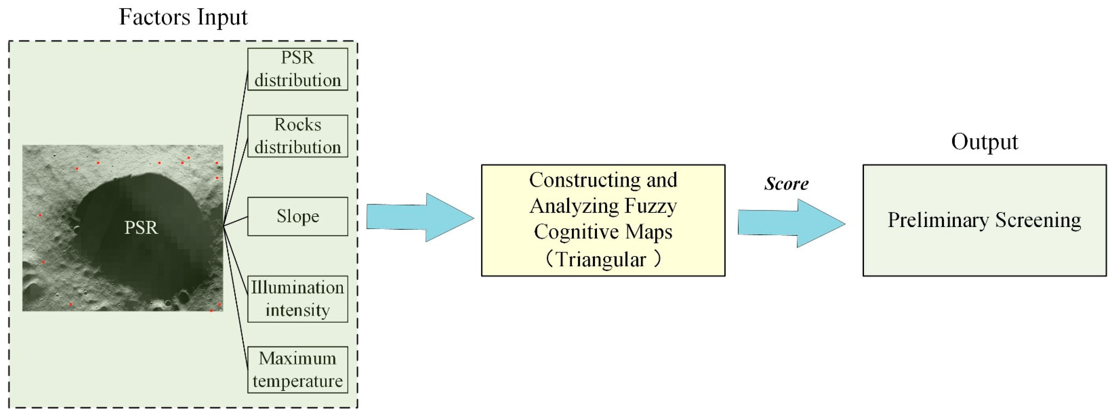
- We investigate the main factors affecting site selection based on analyzing lunar multi-source remote sensing data, combined with previous actual engineering constraints, and preliminary screening of the conditions of future lunar south pole exploration areas.
- A comprehensive multi-factor fuzzy cognition and selection model is proposed to identify landing sites for future missions, combined with score rules, the algorithm quantitatively evaluates three regions (de Gerlache, Shackleton, and Amundsen) and eight sites for other missions subject to a range of engineering constraints and mission requirements.
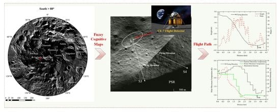
- For the validation results of the model, we take the future CE-7 lunar south pole exploration mission as an example to conduct a route analysis of selected potential landing sites. We analyzed the indicators (slope, light, and temperature) to verify the model’s reliability further.
2. Materials and Methods
2.1. Study Area
2.2. Data
2.3. Methods
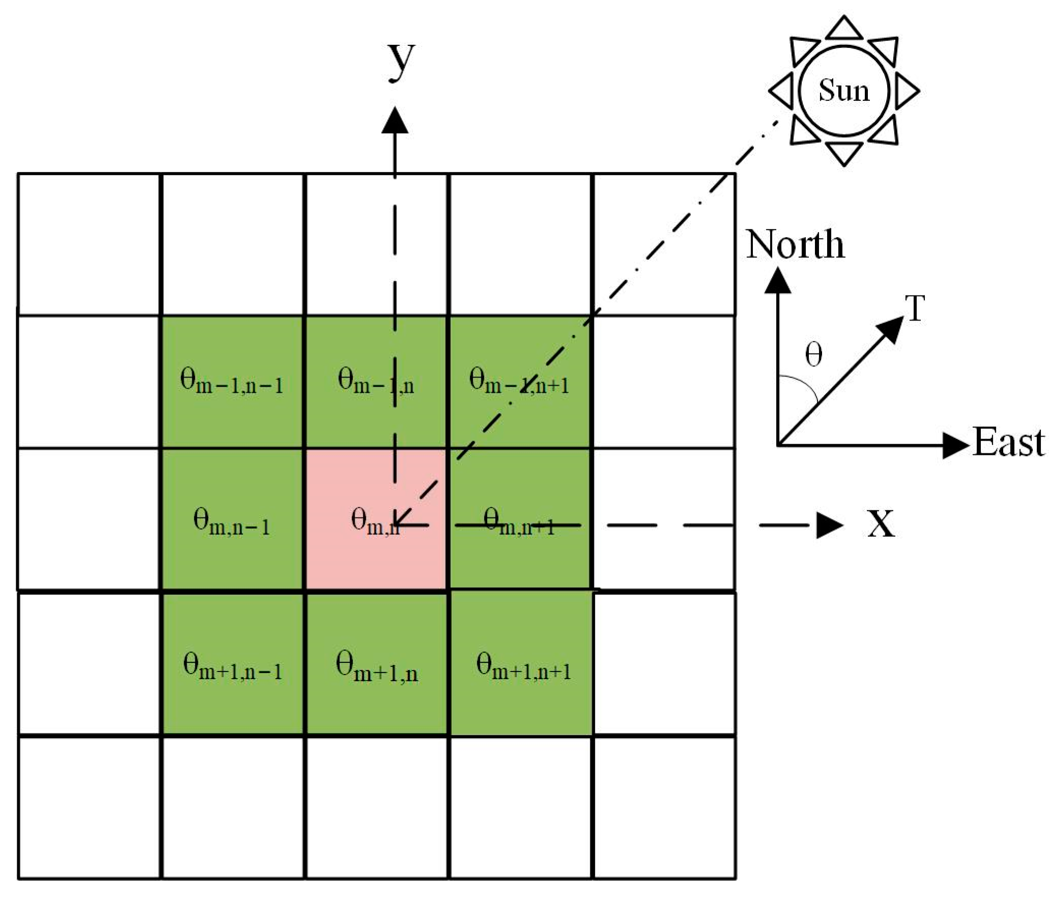
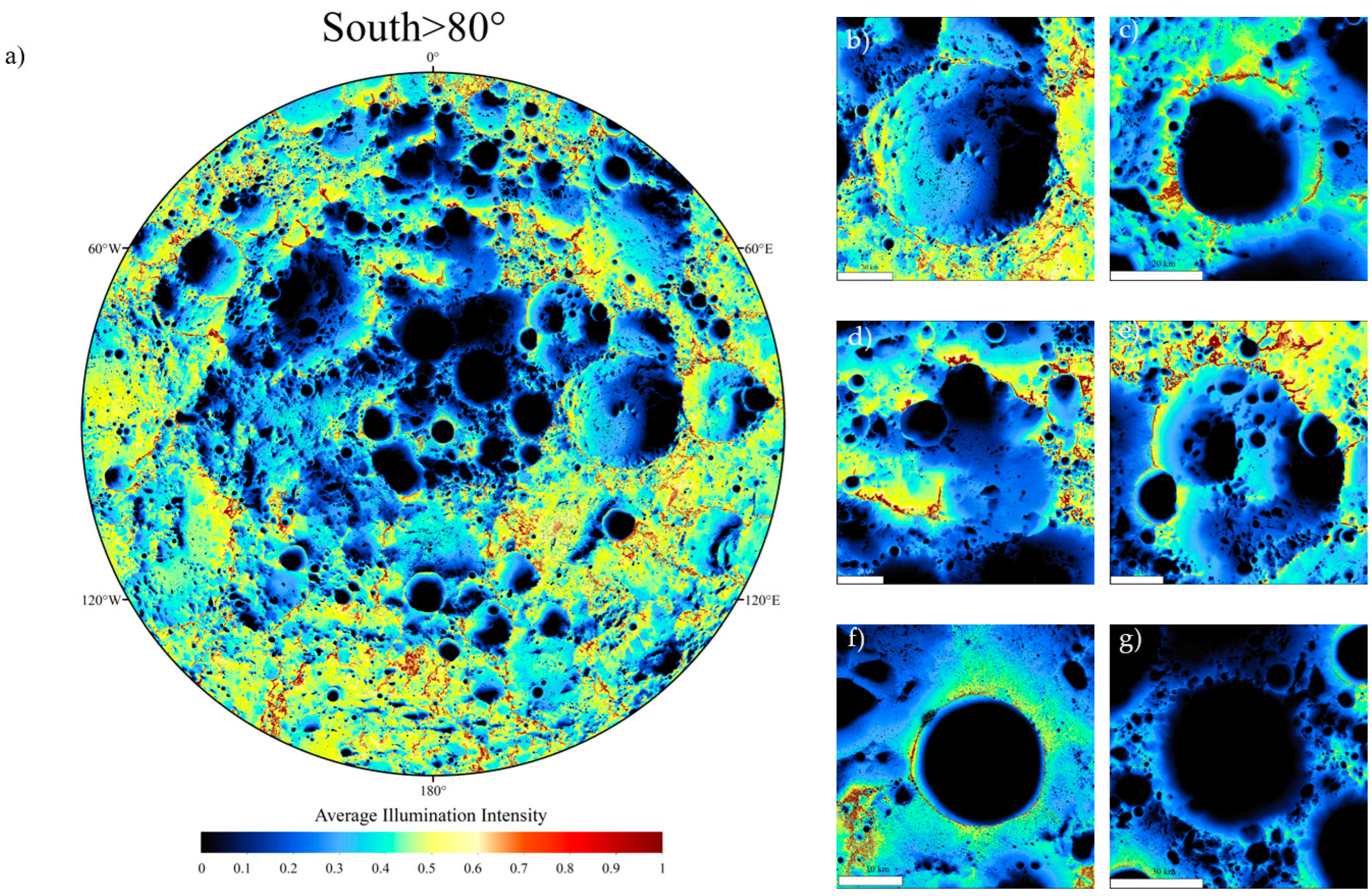
2.3.1. South Pole Illumination Model
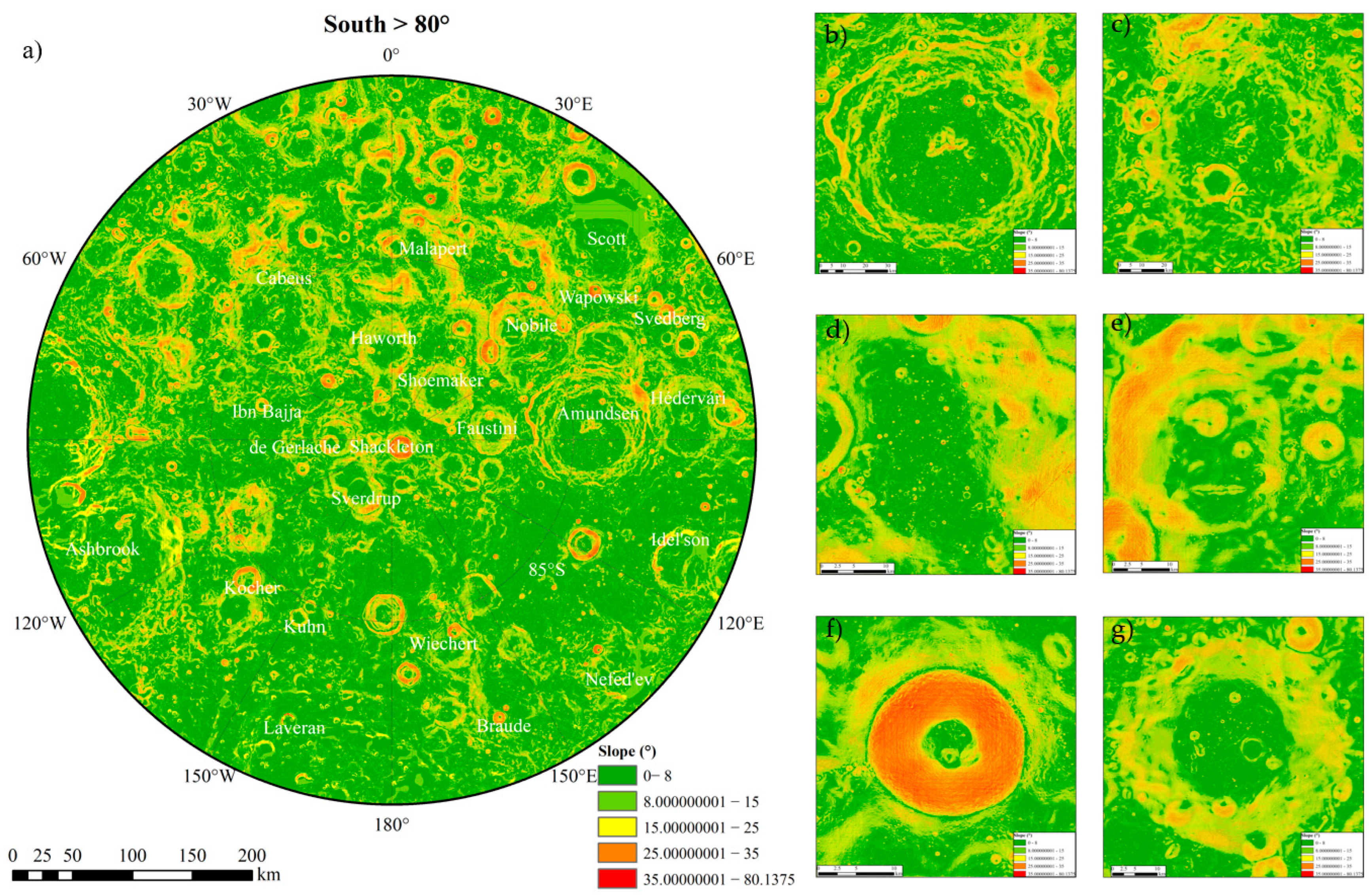
2.3.2. Lunar Surface Slope
2.3.3. Rock Abundance
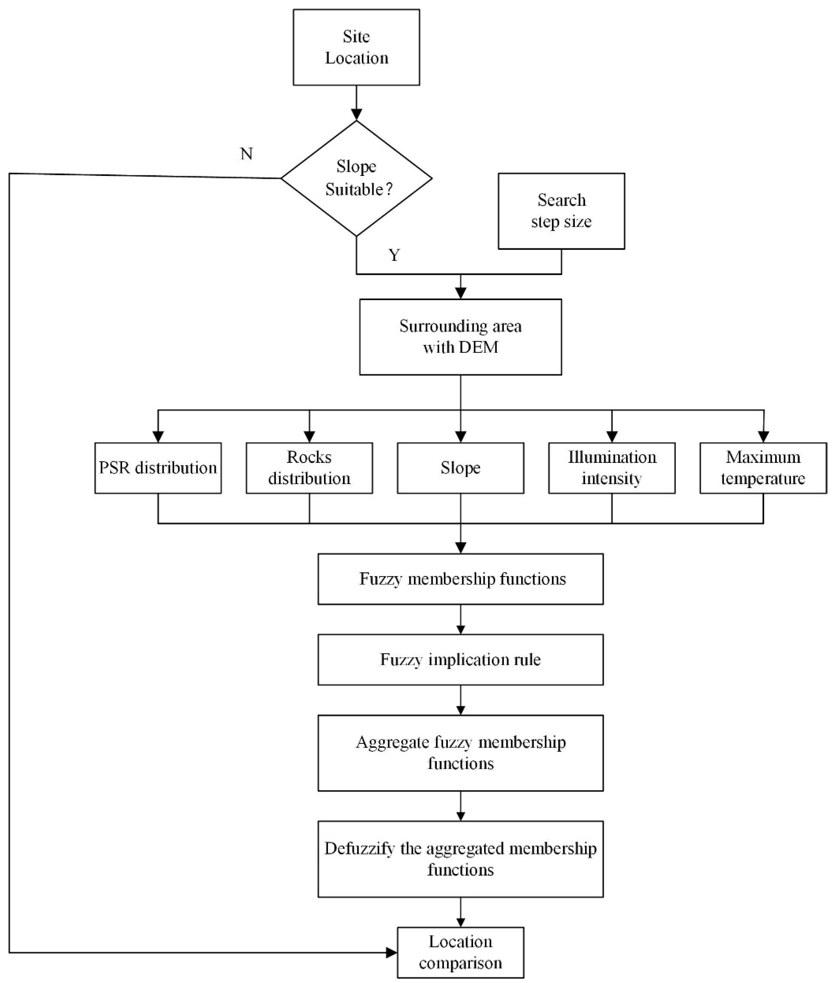
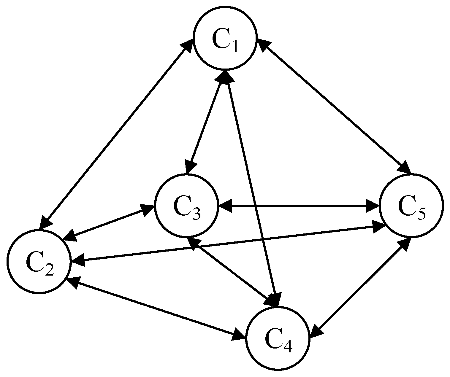
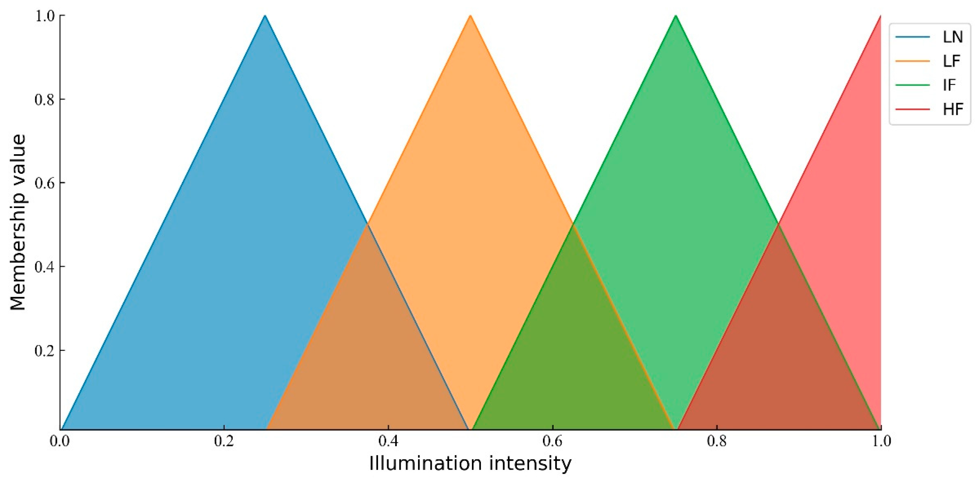
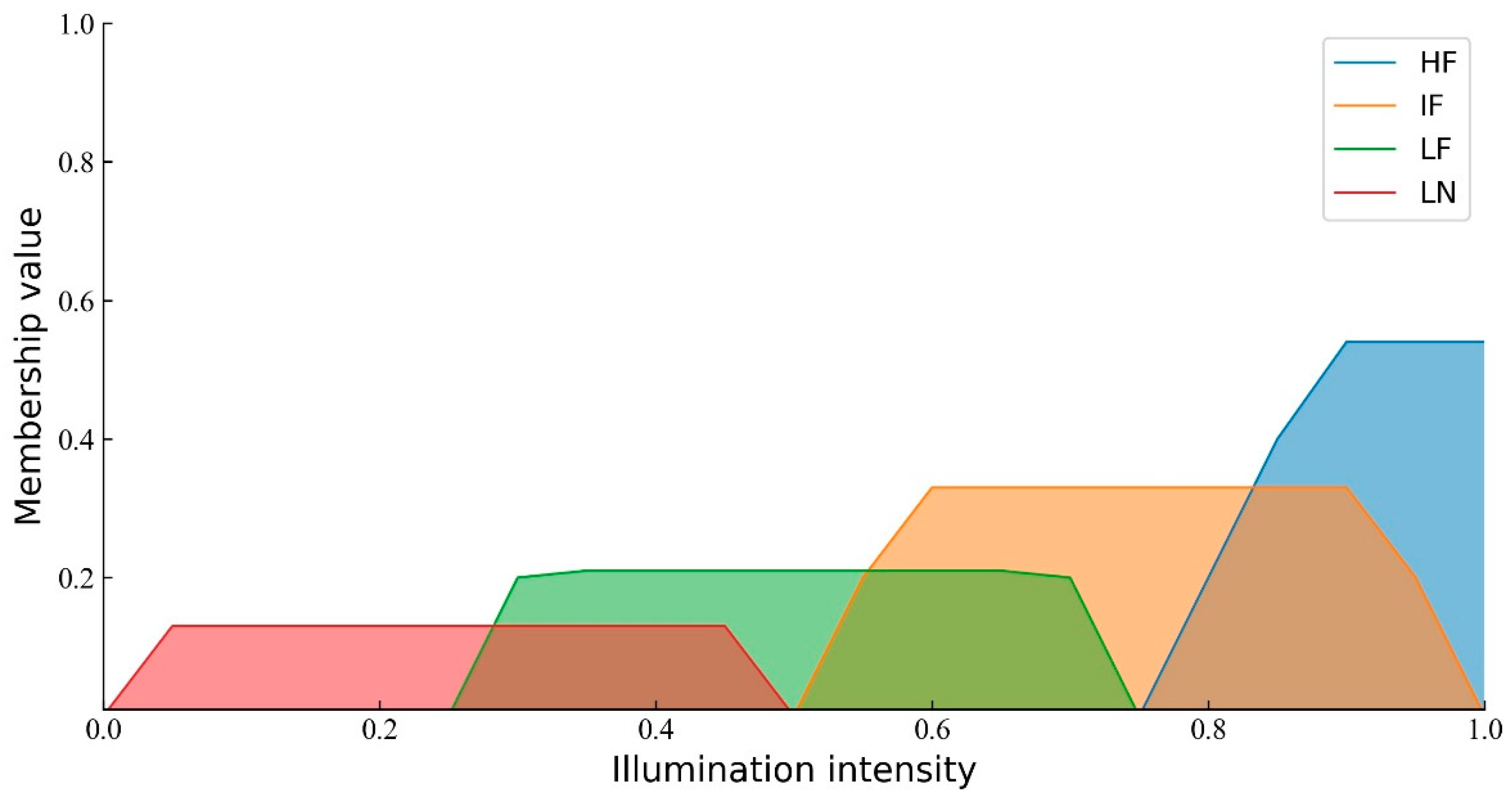
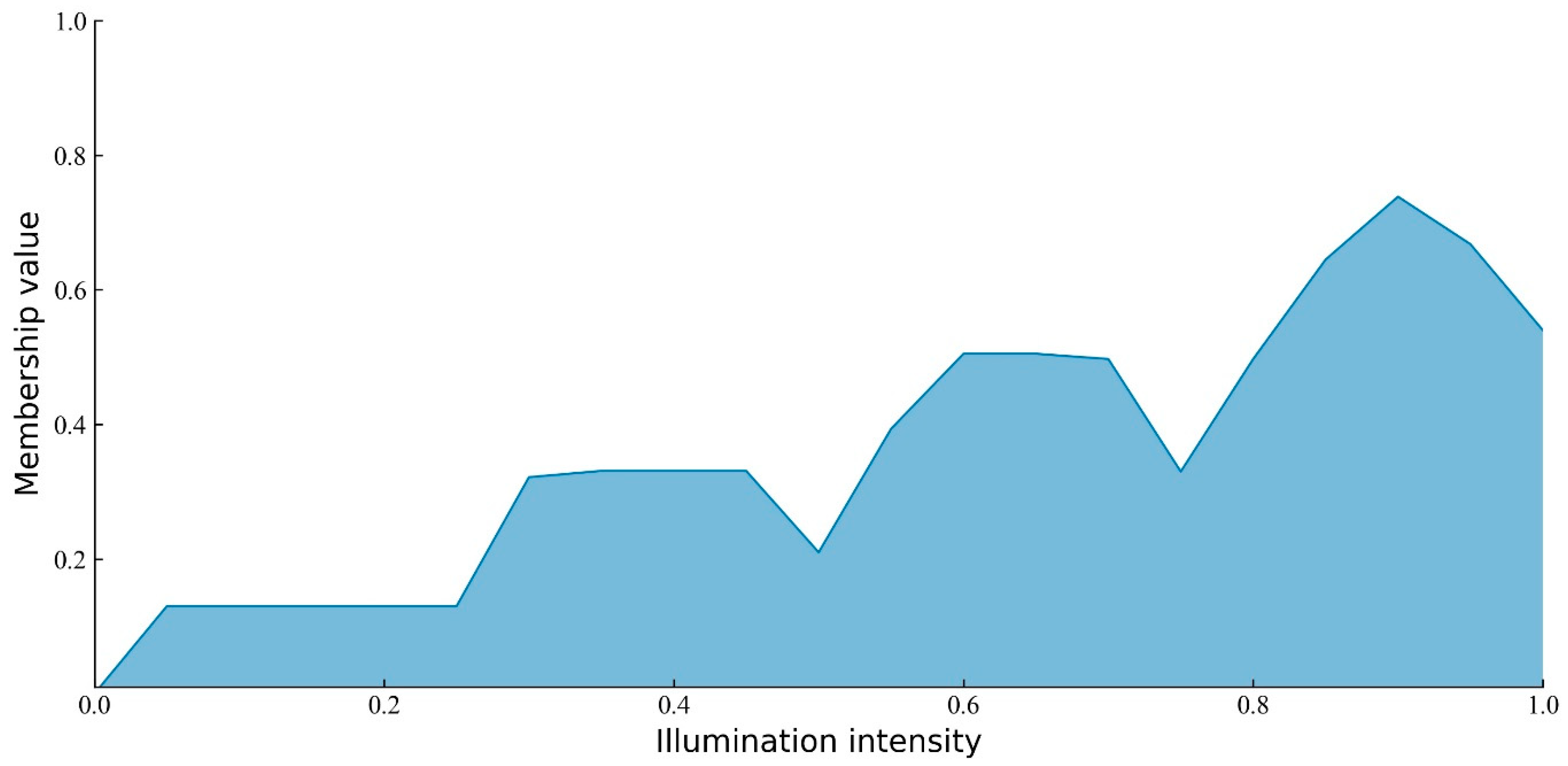
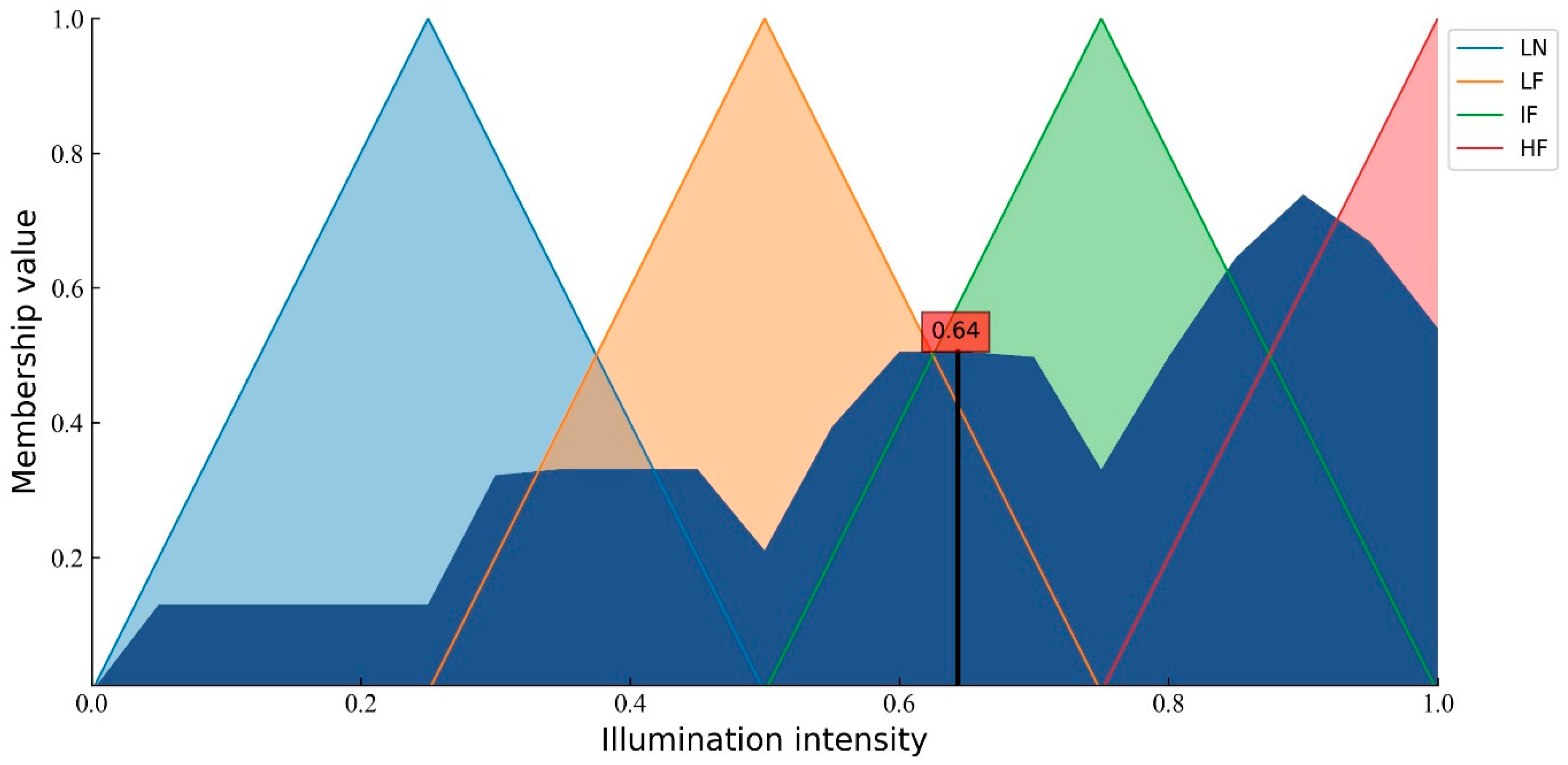
2.3.4. Constructing and Analyzing Fuzzy Cognitive Maps
3. Results and Discussion
3.1. Effects of Permanently Shadowed Regions on Lunar South Pole Siting
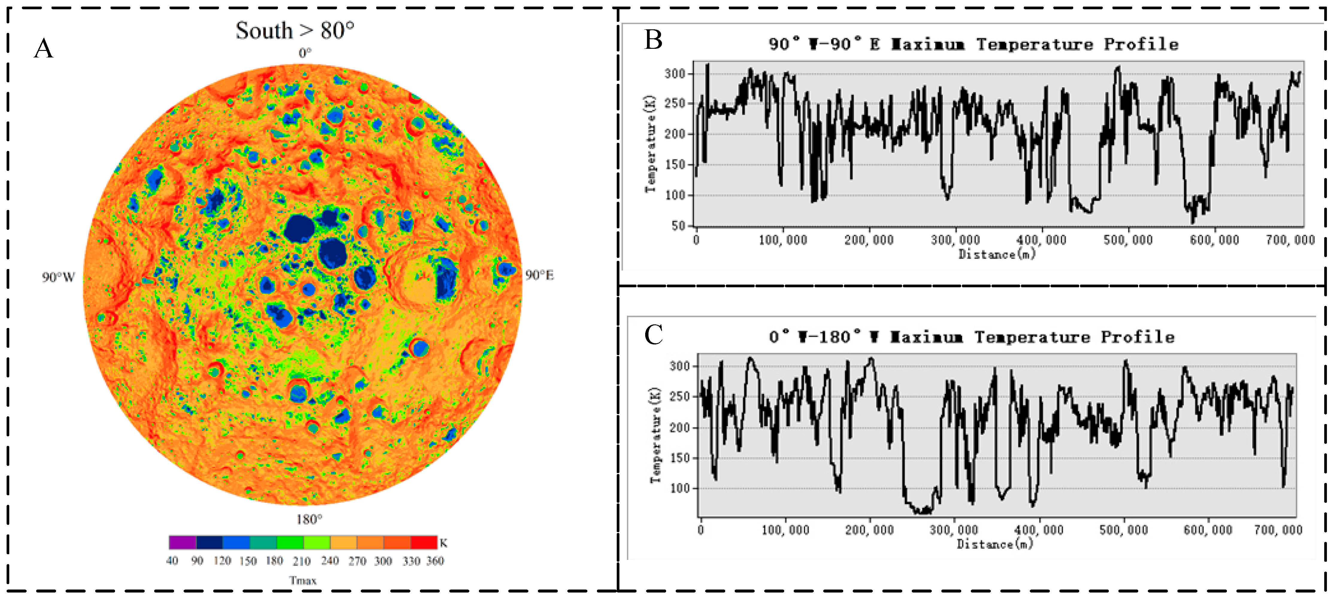
3.2. Influence of Environmental Conditions on the Lunar South Pole Location
3.3. Application of the Proposed Evaluation Model
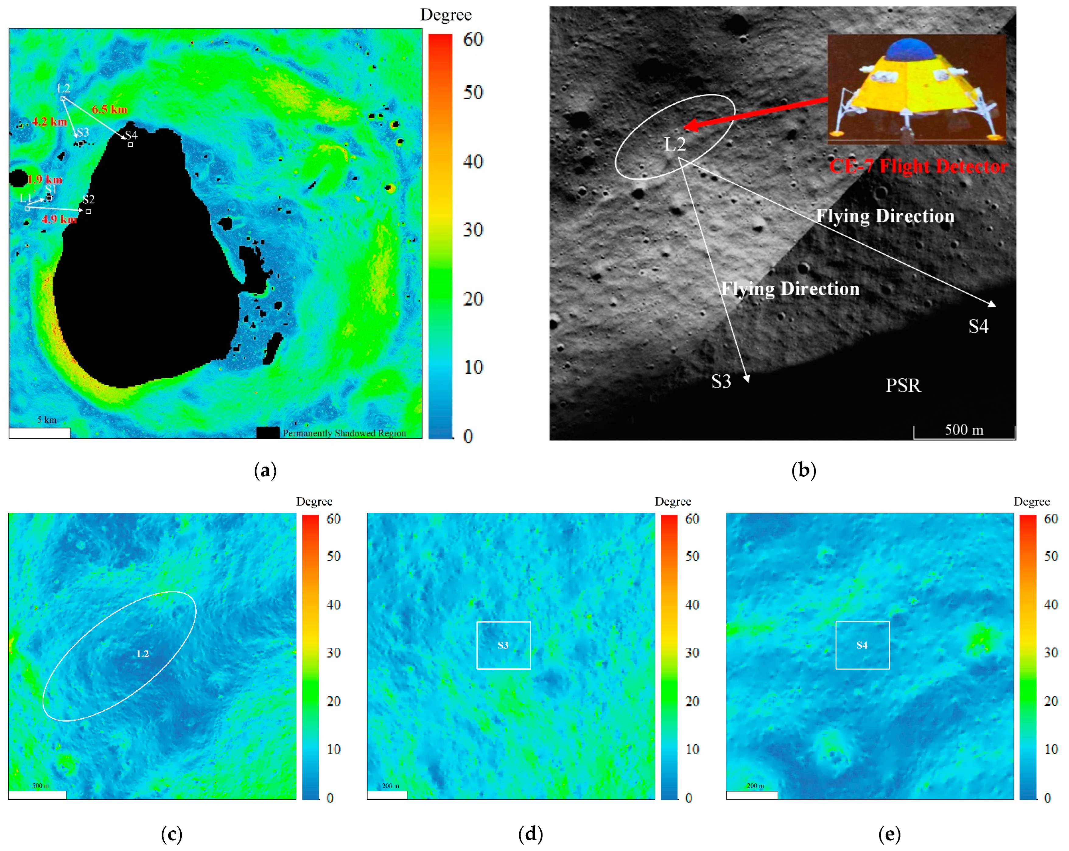
3.4. Route Analysis of Selected Potential Landing Sites
4. Conclusions
Author Contributions
Funding
Data Availability Statement
Acknowledgments
Conflicts of Interest
Abbreviations
| PSRs | Permanently Shadowed Regions |
| CE-7 | Chang ‘E-7 |
| CE-2 | Chang ‘E-2 |
| LOLA | Lunar Orbiter Laser Altimeter |
| NAC | Narrow Angle Camera |
| WAC | Wide Angle Camera |
| LRO | Lunar Reconnaissance Orbiter |
| LROC | Lunar Reconnaissance Orbiter Camera |
| DEM | Digital Elevation Model |
| DOM | Digital Orthophoto Map |
| ROI | Region of Interest |
| LPNS | Prospector Neutron Spectrometer |
| GIS | Geographic Information System |
| CFA | Cumulative Fractional Area |
| FCMs | Fuzzy Cognitive Maps |
| FAM | Fuzzy Allocation Matrix |
References
- Silver, L.T. Uranium-Thorium-Lead Isotope Relations in Lunar Materials. Science 1970, 167, 468–471. [Google Scholar] [CrossRef] [PubMed]
- Liu, J.; Zeng, X.; Li, C.; Ren, X.; Yan, W.; Tan, X.; Zhang, X.; Chen, W.; Zuo, W.; Liu, Y.; et al. Landing Site Selection and Overview of China’s Lunar Landing Missions. Space Sci. Rev. 2021, 217, 6. [Google Scholar] [CrossRef]
- Flahaut, J.; Carpenter, J.; Williams, J.P.; Anand, M.; Zhao, S. Regions of interest (ROI) for future exploration missions to the lunar South Pole. Planet Space Sci. 2019, 180, 104750. [Google Scholar] [CrossRef]
- Korotev, R.L. A Unique Chunk of the Moon. Science 2004, 305, 622–623. [Google Scholar] [CrossRef] [PubMed]
- Schorghofer, N.; Williams, J.P.; Martinez-Camacho, J.; Paige, D.A.; Siegler, M.A. Carbon dioxide cold traps on the Moon. Geophys. Res. Lett. 2021, 48, e2021GL095533. [Google Scholar] [CrossRef]
- Pallava, B. India plans to land near moon’s south pole. Science 2018, 359, 503–504. [Google Scholar] [CrossRef]
- Paige, D.A.; Siegler, M.A.; Zhang, J.A.; Hayne, P.O.; Foote, E.J.; Bennett, K.A.; Vasavada, A.R.; Greenhagen, B.T.; Schofield, J.T.; McCleese, D.J.; et al. Diviner Lunar Radiometer Observations of Cold Traps in the Moon’s South Polar Region. Science 2010, 330, 479–482. [Google Scholar] [CrossRef]
- Hayne, P.O.; Hendrix, A.; Sefton-Nash, E.; Siegler, M.A.; Lucey, P.G.; Retherford, K.D.; Williams, J.-P.; Greenhagen, B.T.; Paige, D.A. Evidence for exposed water ice in the Moon’s south polar regions from Lunar Reconnaissance Orbiter ultraviolet albedo and temperature measurements. Icarus 2015, 255, 58–69. [Google Scholar] [CrossRef]
- Li, S.; Lucey, P.G.; Milliken, R.E.; Hayne, P.O.; Fisher, E.; Williams, J.-P.; Hurley, D.M.; Elphic, R.C. Direct evidence of surface exposed water ice in the lunar polar regions. Proc. Natl. Acad. Sci. USA 2018, 115, 8907–8912. [Google Scholar] [CrossRef]
- Li, C.; Wang, C.; Wei, Y.; Lin, Y. China’s present and future lunar exploration program. Science 2019, 365, 238–239. [Google Scholar] [CrossRef]
- Liu, N.; Jin, Y.Q. Selection of a Landing Site in the Permanently Shadowed Portion of Lunar Polar Regions Using DEM and Mini-RF Data. IEEE Geosci. Remote Sens. Lett. 2022, 19, 1–5. [Google Scholar] [CrossRef]
- Brown, H.M.; Boyd, A.K.; Denevi, B.W.; Henriksen, M.R.; Manheim, M.R.; Robinson, M.S.; Speyerer, E.J.; Wagner, R.V. Resource potential of lunar permanently shadowed regions. Icarus 2022, 377, 114874. [Google Scholar] [CrossRef]
- Basilevsky, A.T.; Krasilnikov, S.S.; Ivanov, M.A.; Malenkov, M.I.; Michael, G.G.; Liu, T.; Head, J.W.; Scott, D.R.; Lark, L. Potential Lunar Base on Mons Malapert: Topographic, Geologic and Trafficability Considerations. Sol. Syst. Res. 2019, 53, 383–398. [Google Scholar] [CrossRef]
- Gawronska, A.J.; Barrett, N.; Boazman, S.J.; Gilmour, C.M.; Kring, D.A. Geologic Context and Potential EVA Targets at the Lunar South Pole. Adv. Space Res. 2020, 66, 1247–1264. [Google Scholar] [CrossRef]
- Heldmann, J.L.; Colaprete, A.; Elphic, R.C.; Bussey, B.; McGovern, A.; Beyer, R.; Leesa, D.; Deansa, M.; Deans, M. Site selection and traverse planning to support a lunar polar rover mission: A case study at Haworth Crater. Acta Astronaut. 2016, 127, 308–320. [Google Scholar] [CrossRef]
- Qiao, L.; Ling, Z.; Head, J.W.; Ivanov, M.A.; Liu, B. Analyses of Lunar Orbiter Laser Altimeter 1,064-nm Albedo in Permanently Shadowed Regions of Polar Crater Flat Floors: Implications for Surface Water Ice Occurrence and Future In Situ Exploration. Earth Space Sci. 2019, 6, 467–488. [Google Scholar] [CrossRef]
- Fisher, E.A.; Lucey, P.G.; Lemelin, M.; Greenhagen, B.T.; Siegler, M.A.; Mazarico, E.; Aharonson, O.; Williams, J.-P.; Hayne, P.O.; Neumann, G.A.; et al. Evidence for surface water ice in the lunar polar regions using reflectance measurements from the Lunar Orbiter Laser Altimeter and temperature measurements from the Diviner Lunar Radiometer Experiment. Icarus 2017, 292, 74–85. [Google Scholar] [CrossRef]
- Lemelin, M.; Blair, D.M.; Roberts, C.E.; Runyon, K.D.; Nowka, D.; Kring, D.A. High-priority lunar landing sites for in situ and sample return studies of polar volatiles. Planet Space Sci. 2014, 101, 149–161. [Google Scholar] [CrossRef]
- Ivanov, M.A.; Hiesinger, H.; van der Bogert, C.H.; Orgel, C.; Pasckert, J.H.; Head, J.W. Geologic History of the Northern Portion of the South Pole-Aitken Basin on the Moon. J. Geophys. Res. Planets 2018, 123, 2585–2612. [Google Scholar] [CrossRef]
- Spudis, P.D.; Bussey, B.; Plescia, J.; Josset, J.-L.; Beauvivre, S. Geology of Shackleton Crater and the south pole of the Moon. Geophys. Res. Lett. 2008, 35, 14. [Google Scholar] [CrossRef] [Green Version]
- Robinson, M.S.; Brylow, S.M.; Tschimmel, M.; Humm, D.; Lawrence, S.J.; Thomas, P.C.; Denevi, B.W.; Bowman-Cisneros, E.; Zerr, J.; Ravine, M.A.; et al. Lunar Reconnaissance Orbiter Camera (LROC) Instrument Overview. Space Sci. Rev. 2010, 150, 81–124. [Google Scholar] [CrossRef]
- Smith, D.E.; Zuber, M.T.; Neumann, G.A.; Mazarico, E.; Lemoine, F.G.; Head Iii, J.W.; Lucey, P.G.; Aharonson, O.; Robinson, M.S.; Sun, X.; et al. Summary of the results from the lunar orbiter laser altimeter after seven years in lunar orbit. Icarus 2017, 283, 70–91. [Google Scholar] [CrossRef]
- Williams, J.P.; Paige, D.A.; Greenhagen, B.T.; Sefton-Nash, E. The global surface temperatures of the Moon as measured by the Diviner Lunar Radiometer Experiment. Icarus 2017, 283, 300–325. [Google Scholar] [CrossRef]
- Shoemaker, E.M.; Robinson, M.S.; Eliason, E.M. The South Pole Region of the Moon as Seen by Clementine. Science 1994, 266, 1851–1854. [Google Scholar] [CrossRef] [PubMed]
- Mazarico, E.; Neumann, G.A.; Smith, D.E.; Zuber, M.T.; Torrence, M.H. Illumination conditions of the lunar polar regions using LOLA topography. Icarus 2011, 211, 1066–1081. [Google Scholar] [CrossRef]
- Gläser, P.; Scholten, F.; Rosa, D.D.; Figuera, R.M.; Oberst, J.; Mazarico, E.; Neumann, G.A.; Robinson, M.S. Illumination conditions at the lunar south pole using high resolution Digital Terrain Models from LOLA. Icarus 2014, 243, 78–90. [Google Scholar] [CrossRef]
- Kneissl, T.; Neukum, S.V.G.G. Map-projection-independent crater size-frequency determination in GIS environments—New software tool for ArcGIS. Planet Space Sci. 2011, 59, 1243–1254. [Google Scholar] [CrossRef]
- Watkins, R.N.; Jolliff, B.L.; Mistick, K.; Fogerty, C.; Lawrence, S.J.; Singer, K.N.; Ghent, R.R. Boulder Distributions Around Young, Small Lunar Impact Craters and Implications for Regolith Production Rates and Landing Site Safety. J. Geophys. Res. Planets 2019, 124, 2754–2771. [Google Scholar] [CrossRef]
- Li, Y.; Wu, B. Analysis of Rock Abundance on Lunar Surface from Orbital and Descent Images Using Automatic Rock Detection. J. Geophys. Res. Planets 2018, 123, 1061–1088. [Google Scholar] [CrossRef]
- Kosko, B. Fuzzy cognitive maps. Int. J. Man Mach. Stud. 1986, 21, 65–76. [Google Scholar] [CrossRef]
- Stylios, C.D.; Groumpos, P.P. Modeling complex systems using fuzzy cognitive maps. IEEE Trans. Syst. Man Cybern. Part A Syst. Hum. 2004, 34, 155–162. [Google Scholar] [CrossRef]
- Nápoles, G.; Espinosa, M.L.; Grau, I.; Vanhoof, K. FCM Expert: Software Tool for Scenario Analysis and Pattern Classification Based on Fuzzy Cognitive Maps. Int. J. Artif. Intell. Tools 2018, 27, 1793–6349. [Google Scholar] [CrossRef]
- Mkhitaryan, S.; Giabbanelli, P.J.; Vries, N.; Crutzen, R. Dealing with complexity: How to use a hybrid approach to incorporate complexity in health behavior interventions. Intell. Based Med. 2020, 12, 100008. [Google Scholar] [CrossRef]
- Zhang, K. Influence of Topography on the Site Selection of a Moon-Based Earth Observation Station. Sensors 2021, 21, 7198. [Google Scholar] [CrossRef]
- Chen, J.; Zhao, S.; Gao, T.; Yuzeng, X.U.; Zhang, L.; Ding, Y.; Zhang, X.; Zhao, Y.; Hou, G. High-efficiency Monocrystalline Silicon Solar Cells:Development Trends and Prospects. Mater. Rep. 2019, 12, 1168. [Google Scholar]
- Yang, Z.; Liu, J. Learning fuzzy cognitive maps with convergence using a multi-agent genetic algorithm. Soft Comput. 2020, 24, 4055–4066. [Google Scholar] [CrossRef]
- Stach, W.; Kurgan, L.; Pedrycz, W.; Reformat, M. Genetic learning of fuzzy cognitive maps. Fuzzy Sets Syst. 2005, 153, 371–401. [Google Scholar] [CrossRef]
- Salmeron, J.L.; Papageorgiou, E.I. A fuzzy grey cognitive maps-based decision support system for radiotherapy treatment planning. Knowl. Based Syst. 2012, 30, 151–160. [Google Scholar] [CrossRef]
- Noda, H.; Araki, H.; Goossens, S.; Ishihara, Y.; Matsumoto, K.; Tazawa, S.; Kawano, N.; Sasaki, S. Illumination conditions at the lunar polar regions by KAGUYA(SELENE) laser altimeter. Geophys. Res. Lett. 2008, 35, 24. [Google Scholar] [CrossRef]
- Speyerer, E.J.; Robinson, M.S. Persistently illuminated regions at the lunar poles: Ideal sites for future exploration. Icarus 2013, 222, 122–136. [Google Scholar] [CrossRef]
- Williams, J.-P.; Greenhagen, B.T.; Paige, D.A.; Schorghofer, N.; Sefton-Nash, E.; Hayne, P.O.; Lucey, P.G.; Siegler, M.A.; Aye, K.M. Seasonal Polar Temperatures on the Moon. J. Geophys. Res. Planets 2019, 124, 2505–2521. [Google Scholar] [CrossRef]


| Spacecraft | Payload | Data Type | Resolution | Range | Application Section | Projection Method |
|---|---|---|---|---|---|---|
| CE-2 | CCD | DEM | 20 m/pixel | 80°S–90°S | 2.3.2/3.2 | Polar stereographic projection |
| DOM | 7 m/pixel | Local area | 2.1/3.3 | |||
| LRO | LROC | Images | 1 m/pixel | Local area | 2.3.3/3.4 | |
| LOLA | DEM | 5 m/pixel | Local area | 3.4 | ||
| 240 m/pixel | 75°S–90°S | 2.3.1/3.2 | ||||
| Diviner | Thermal infrared | 200 m/pixel | 80°S–90°S | 3.2 |
| Restrictive Factors | Significance Ordering | ||
|---|---|---|---|
| Scientific Targets | PSR | Square measure | 1 |
| Environmental conditions | Slope | 2–10 m baseline | 2 |
| Rock distribution | Rock abundance | 3 | |
| Illumination condition | Illumination intensity | 4 | |
| Surface thermal environment | Temperature | 5 | |
| Name | Pit Area | Maximum Slope | Minimum Slope | Average Slope | Ratio Less Than 8° |
|---|---|---|---|---|---|
| Amundsen | 2500 km2 | 77° | 0.4° | 10° | 48% |
| de Gerlache | 49 km2 | 61.5° | 0.9° | 15.4° | 27% |
| Malapert | 490 km2 | 63° | 1.3° | 8.7° | 57% |
| Nobile | 260 km2 | 64° | 1.2° | 14° | 27% |
| Shackleton | 37 km2 | 62.5° | 0° | 23° | 12% |
| Shoemaker | 603 km2 | 65.3° | 0° | 11.6° | 35% |
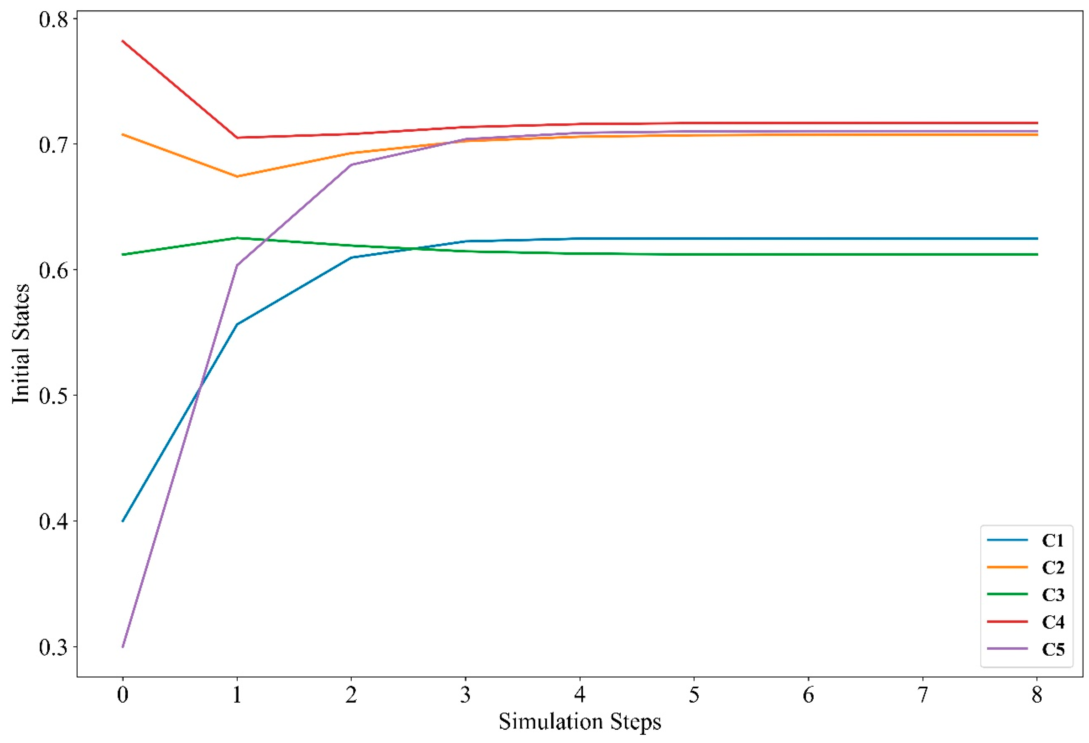
| Node | C1 | C2 | C3 | C4 | C5 |
|---|---|---|---|---|---|
| Initial value | 0.412 | 0.707 | 0.607 | 0.783 | 0.314 |
| Stable value | 0.624 | 0.698 | 0.581 | 0.714 | 0.701 |
| Difference value | 0.212 | 0.009 | 0.026 | 0.069 | 0.387 |
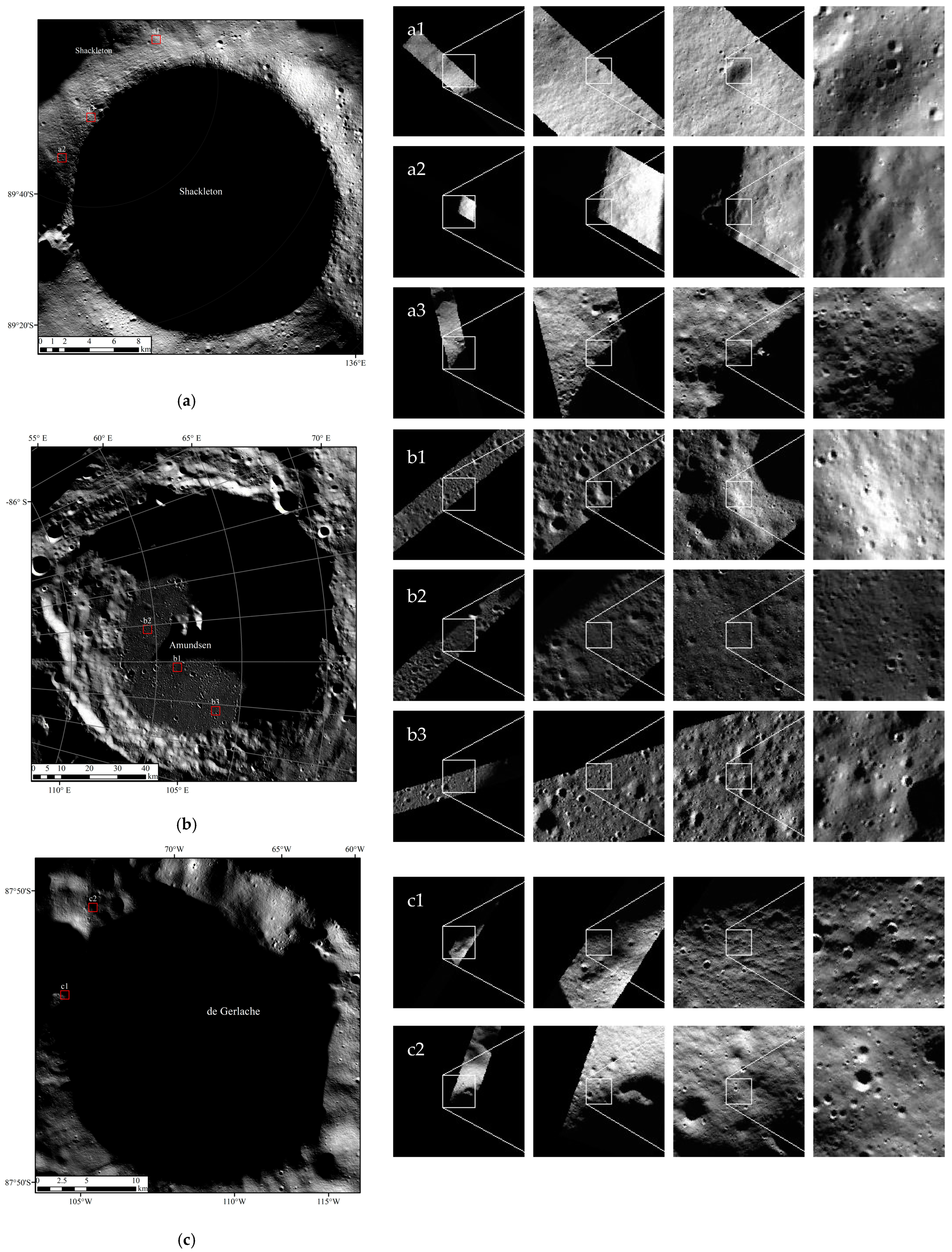
| Shackleton | Amundsen | de Gerlache | ||||||
|---|---|---|---|---|---|---|---|---|
| ROI | a1 | a2 | a3 | b1 | b2 | b3 | c1 | c2 |
| Latitude | 89.793°S | 89.782°S | 89.961°S | 84.735°S | 85.129°S | 84.253°S | 87.984°S | 88.035°S |
| Longitude | 26.73°E | 156.36°W | 145.25°W | 90.82°E | 85.61°E | 95.78°E | 86.01°W | 77.25°W |
| Slope | 7.9° | 7.3° | 2.2° | 0.6° | 1.3° | 3.1° | 5.3° | 4.1° |
| Rocks distribution | 11.7% | 7.8% | 8.3% | 7.2% | 9.2% | 8.5% | 6.8% | 2.6% |
| Average illumination intensity | 41.53% | 51.91% | 52.73% | 30.51% | 27.41% | 25.27% | 42.12% | 50.14% |
| Average maximum temperature | 147 K | 131K | 151 K | 85K | 104K | 96K | 113K | 146k |
| Score | 0.736 | 0.745 | 0.814 | 0.784 | 0.701 | 0.651 | 0.758 | 0.816 |
Publisher’s Note: MDPI stays neutral with regard to jurisdictional claims in published maps and institutional affiliations. |
© 2022 by the authors. Licensee MDPI, Basel, Switzerland. This article is an open access article distributed under the terms and conditions of the Creative Commons Attribution (CC BY) license (https://creativecommons.org/licenses/by/4.0/).
Share and Cite
Jia, Y.; Liu, L.; Wang, X.; Guo, N.; Wan, G. Selection of Lunar South Pole Landing Site Based on Constructing and Analyzing Fuzzy Cognitive Maps. Remote Sens. 2022, 14, 4863. https://doi.org/10.3390/rs14194863
Jia Y, Liu L, Wang X, Guo N, Wan G. Selection of Lunar South Pole Landing Site Based on Constructing and Analyzing Fuzzy Cognitive Maps. Remote Sensing. 2022; 14(19):4863. https://doi.org/10.3390/rs14194863
Chicago/Turabian StyleJia, Yutong, Lei Liu, Xingchen Wang, Ningbo Guo, and Gang Wan. 2022. "Selection of Lunar South Pole Landing Site Based on Constructing and Analyzing Fuzzy Cognitive Maps" Remote Sensing 14, no. 19: 4863. https://doi.org/10.3390/rs14194863
APA StyleJia, Y., Liu, L., Wang, X., Guo, N., & Wan, G. (2022). Selection of Lunar South Pole Landing Site Based on Constructing and Analyzing Fuzzy Cognitive Maps. Remote Sensing, 14(19), 4863. https://doi.org/10.3390/rs14194863