Abstract
Floods are one of the most destructive natural hazards to which Australia is exposed. The frequency of extreme rainfall events and consequential floods are projected to increase into the future as a result of anthropogenic climate change. This highlights the need for more holistic risk assessments of flood affected regions. Flood risk assessments (FRAs) are used to inform decision makers and stakeholders when creating mitigation and adaptation strategies for at-risk communities. When assessing flood risk, previous FRAs from Australia’s most flood prone regions were generally focused on the flood hazard itself, and rarely considering flood vulnerability (FV). This study assessed FV in one of Australia’s most flood prone regions—the Hawkesbury-Nepean catchment, and investigated indicator-based approaches as a proxy method for Australian FV assessment instead of hydrological modelling. Four indicators were selected with the intention of representing environmental and socio-economic characteristics: elevation, degree of slope, index of relative socio-economic disadvantage (IRSD), and hydrologic soil groups (HSGs). It was found that combination of low elevation, low degree of slope, low IRSD score, and very-low infiltration soils resulted in very high levels of vulnerability. FV was shown to be at its highest in the Hawkesbury-Nepean valley flood plain region on the outskirts of Greater Western Sydney, particularly in Blacktown, Penrith, and Liverpool. This actionable risk data which resulted from the final FV index supported the practicality and serviceability of the proxy indicator-based approach. The developed methodology for FV assessment is replicable and has the potential to help inform decision makers of flood-prone communities in Australia, particularly in data scarce areas.
1. Introduction
The implications of natural hazards, including floods have become increasingly profound in Australia, as well as globally over the past few decades. The ensuing impacts of such events on communities are extensive and underscore the need for more proactive approaches to natural hazard risk mitigation and adaptation [1]. A flood is described by the Australian Bureau of Meteorology (BoM) as the “overflow of water beyond the normal limits of a watercourse” [2]. Notably over the past years, the effects of several flood disasters have been felt in regions along Australia’s East Coast. Historically, flood events have been recurring in Queensland and New South Wales [3], however their increasing frequency and intensity has caused concern amongst the communities most affected by them.
Ecologically, floods have the ability to be beneficial in environments that regularly endure them. In floodplain ecosystems that are largely undisturbed, the exposure to annual or occasional extreme floods can see benefits such as the dispersal of soil nutrients and sediments [4]. However, in modern times, urbanisation on these flood plains has meant that natural ecosystems are largely fragmented or lost completely [4,5]. When replaced with human settlements, flood events become devastating, causing the loss of important infrastructure, homes, and lives [6]. According to the EMT-DAT Natural Disaster Database, floods were recorded globally as the most frequent natural disaster (43%) between 1997 and 2013 [7]. They are also estimated as one of the costliest occurring natural hazards in Australia [8], with the Australian Insurance Council estimating that in 2022 alone, floods have caused AUD 4.3 billion in insured losses [9].
Floods are commonly categorised under three main classifications: pluvial, fluvial, and coastal. Pluvial floods which are the result of rainfall events are considered surface water floods or ‘flash floods’, whereas fluvial floods are defined as the overflowing of a river or water body. Coastal flooding often involves the surge of seawater onto land from events such as storms [10]. For the purposes of this study, pluvial and fluvial flooding will be the main focus.
Interannual variability in the frequency and intensity of floods in Australia is influenced by a number of climate drivers including the El Niño-Southern Oscillation (ENSO) which contains the cooler, wetter La Niña phase, contributes largely to the heavy precipitation events that often lead to Australian floods [11]. Anthropogenic climate change coupled with influence of the ENSO and other key climate drivers can culminate in an intensified hydrological cycle, resulting in extreme rainfall events particularly in Southern Queensland (QLD) and along the New South Wales (NSW) coast [12].
Globally, there has been increasing endeavours within the scientific community to develop methods to assess potential natural disaster risks [13]. Natural hazard risk assessments aim to gauge the potential threats posed by a natural disaster to a community. Risk is usually described as “the probability of a loss” as a product of three risk components—hazard, exposure, and vulnerability [14,15]. and can be expressed as Equation (1):
Risk = hazard × exposure × vulnerability
The current approach to flood risk assessment (FRA) and management in Australia is customarily conducted on a local government area (LGA) level. The methodology of FRA in these cases is widely variable as well as sparse, and largely hazard-centric [16,17]. Currently, the dominant process of FRA across Australian LGAs involves hydrological modelling and mapping using remote sensing and Geographical Information Systems (GIS) software to understand flood behaviour and characteristics [18]. This has left some disparity in the consideration of how hazard, exposure, and vulnerability constitute flood risk, and in particular how pre-existing conditions may lessen or heighten losses due to flooding [19]. Flood modelling assessments of this design are usually completed in accordance with the Australian Institute of Disaster Resilience guidelines for flood risk management [20]. By following this guideline, LGA reports can be heavily centred around hazard modelling and can lack a holistic perspective in the sense of models including the three factors (hazard, exposure, and vulnerability).
In comparison, another methodology that has been used internationally to assess flood risk is the use of indices. Index-based assessment and mapping condenses large datasets into single values that can be applied to features across a study area. This scalable and replicable proxy methodology of FRA is quantitative in nature and encourages a more holistic approach to assessments [21].
This study focuses specifically on flood vulnerability (FV) as one of three risk components, and how the antecedent conditions within a given area affect the outcome of a flood event within communities. The definition of FV is varied in the literature, so for this study the definition provided by the Intergovernmental Panel on Climate Change (IPCC) was used. The IPCC defines vulnerability as “the propensity or predisposition to be adversely affected. It encompasses a variety of concepts and elements, including sensitivity or susceptibility to harm and lack of capacity to cope and adapt” [14].
It is important to note that the concept of FV often overlaps with that of community flood resilience (CFR). Drawing distinction between these two ideas can be difficult, and literature has underscored this need for correct characterisation. For this study, the IPCC definition was adopted. According to the IPCC, resilience is “the ability of a system and its component parts to anticipate, absorb, accommodate, or recover from the effects of a hazardous event in a timely and efficient manner, including through ensuring the preservation, restoration, or improvement of its essential basic structures and functions” [14]. Literature such as Batica and Gourbesville (2020) [22], outlines that FV encompasses pre-flood event conditions, whereas in contrast, CFR is characterised by actions related to preparedness, response and recovery post-flood event that decrease vulnerability into the future. CFR is an important concept that will be covered in our future investigations. However, in this study, scope will be limited to investigating FV.
In international literature, three main categories are usually considered when assessing FV.
- Physical/environmental: Focuses on coupled human-environmental systems. This aspect delves into the surrounding physical characteristics of an area. This can vary from anthropogenically made places to local ecology [23].
- Social: The product of social inequalities in a given region. These can include gender, ethnicity, age groups, poverty, health, education, marginalised groups, availability of affordable housing, etc. [24,25].
- Economic: Refers to economic assets of a household or community as well as the economic susceptibility of a given place. This can include construction density, retail density, living resources such as food, appliances, private housing, and other commodities [24,25].
In Australia, FV is sparsely included in FRAs. When FV does appear in assessments, it tends to address only one or two of the three FV categories (physical, social and economic), and very rarely draws comparison between factors from each of these categories [26]. This is largely due to community reports by councils or consultancy groups focusing time and resource allocation into hydrological modeling-based approaches [27]. In Australia, FV assessments are predominantly assessed using flood damage models. For this reason, there is room in Australian FRAs for a more holistic, index-based methodology, especially when measuring FV [21].
The Australian FV assessments that do exist infrequently use indicator-based approaches. Indicator methods usually follow a multi-criteria analysis structure that explicitly evaluates multiple conflicting components in decision making. Indicator methods convert geospatial data into standardised indicators with the end goal of producing the final Flood Vulnerability Index (FVI). Internationally, Nasiri et al. (2016) [28] outlines two main approaches to indicator methodology as the deductive and inductive approaches. The deductive approach is built on a theoretical framework and requires considering each indicator relationship with FV. Meanwhile, the inductive approach selects indicators based on statistical links with observed vulnerability consequences. This study adopts a deductive approach in order to properly consider the contribution of each indicator to the vulnerability in the study area. In areas where data can be scarce, or where multiple LGAs must be measured, this index technique can be beneficial as it is scalable and requires less resources than data modeling.
The overall aim of this study is to quantify FV across one of the most flood prone areas in Australia, the Hawkesbury-Nepean catchment (HNC) through a proxy indicator-based approach, and to develop a FVI composed of relevant and specific FV indicators.
2. Materials and Methods
2.1. Study Area
Eastern parts of Australia including Southern Queensland and New South Wales have long been known as areas that are exposed to extreme flood events [29]. In this study, FV to pluvial and fluvial flooding is assessed, meaning that an area that is removed from potential coastal flood events was preferable as a study area. Over the past years, the HNC area located in Greater Western Sydney (GWS) has been subjected to heavy precipitation events that have led to several floods [30]. The region stretches over 21,000 km2 from south of Goulburn to north of the Putty Valley, and from west of Lithgow to the coast. The catchment contains 26 LGAs (Figure 1) and 11 main rivers (Figure 2).
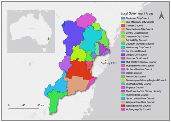
Figure 1.
Local government areas located within the Hawkesbury-Nepean catchment as of 2022.
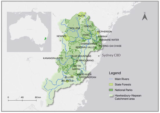
Figure 2.
Map of the Hawkesbury-Nepean catchment area including both national and state parks as well as the main rivers located throughout the catchment as of 2022.
Additionally, the presence of urbanised communities and infrastructure throughout the floodplain means that the effects of flood can have a heightened human impact. This is because there is more that stands to be lost. The severity and frequency of floods in this area, coupled with the tragic losses that have been associated with these events, are important reasons as to why the location was chosen as a case study area.
2.2. Selecting Vulnerability Indicators
The selection of vulnerability indicators was carried out by consulting prior literature and FV assessments. Previous Australian assessments tended to largely focus on either physical or economic indicators, with few using a combination of both. In many cases, flood risk management strategies do not investigate soil structure, which is highlighted in Alaoui et al. (2018) [31] as being a key driver in flood runoff behaviour [1]. International studies showed a more holistic approach to this selection process, with a larger number of assessments using a combination of all three categories outlined above. For this study, this holistic approach is preferable, therefore in the selection process of indicators all three of the vulnerability categories were included in the chosen indicators.
Initially, indicators such as vegetation biomass, topographic wetness index (TWI), and soil curve number (CN) were all considered for physical gauges of the catchment. This was mainly due to data availability, data overlaps, and subjectivity. It was important for this study to be easily replicable in other areas of Australia, and in order to ensure this, the indicators selected must have data availability across the whole country. While vegetation indicators were found to be important in runoff behaviour, they were ruled out as their data availability was inconsistent and hard to obtain in a high resolution. TWI was ruled out due to some overlap with soil moisture indicators in a partnering flood hazard study. The goal of this study involved combining FV with flood hazard to create an index, and the crossover between data here would have rendered the indicator obsolete. Lastly, CN was discarded as the process of its calculation relies on deciphering different land use types present in a given area. This is achieved by consulting a CN table which requires decisions about the cover type and urbanisation characteristics of a given area. Available data on the HNC would not have been informative or sufficient enough to make objective decisions about these properties. Instead, a more unbiased approach was favoured. It was found to be advantageous to limit the number of indicators to three or four in order to preserve simplicity and to reduce overlap, therefore the selection of indicators had to be carefully considered. The following section explains the selected indicators and their relevance to FV.
2.2.1. Elevation
Elevation is a topographic factor that influences the direction and velocity of water flow during flooding. As a physical indicator, elevation shows vulnerability where the lowest lying areas occur as water flows from higher to lower elevated areas. It is expected that the floodplains within the catchment will be the locally lowest lying areas, meaning that they will be the most vulnerable to flood conditions. Earlier studies highlight the use of elevation as a key flood vulnerability indicator [28,32]. While elevation can be a major factor, other factors could be also important, e.g., gradient or the geomorphic character of the study region and subregions which dictate where water flows from and where it flows to. However, being an obvious factor contributing to FV, using elevation data is useful to draw comparisons to the variation in other environmental indicators.
2.2.2. Degree of Slope
Often found coupled with elevation, the degree of slope is the percentage of change in elevation over a certain distance [33]. It describes the shape and relief of the land as opposed to the height of the land. Slope is calculated using Equation (2):
Slope = Difference in height/Horizontal Distance
Slope influences the speed at which water will travel, meaning that in areas with a higher degree of slope, water will runoff more readily resulting in a lower flood risk [34]. This indicator was chosen as it complements elevation data and shows reasonable variation across the catchment. It is also frequently used in past FV assessments with a historically high influence on flood runoff behaviour [35].
2.2.3. Index of Relative Socio-Economic Disadvantage
The Index of Relative Socio-economic Disadvantage (IRSD) is a comprehensive index which is a component of the Socio-Economic Indexes for Areas (SEIFA) created by the Australian Bureau of Statistics (ABS). It summarises a range of information about the economic and social conditions of people and households within an area [36]. Unlike the other indexes, IRSD only describes factors of relative disadvantage, meaning that it purely characterises the pre-flood conditions that make the community most vulnerable. The IRSD was advantageous to adopt as it encompasses both economic and social elements outlined previously, combining two important vulnerability categories into one indicator. IRSD scores are mapped using quintiles. The lowest scoring 20% of areas are given a quintile number of 1, the second-lowest 20% of areas are given a quintile number of 2 and so on, up to the highest 20% of areas which are given a quintile number of 5. Low IRSD scores indicate that an area has a relatively greater disadvantage in general. For example, areas that have low IRSD scores may have (i) many households with low incomes, or (ii) many people with long term health conditions or disabilities, or (iii) many dwellings that are overcrowded, etc. Conversely, areas with a high IRSD score would present a lack of disadvantage meaning, e.g., (i) few households with low incomes, or (ii) few people with long term health conditions or disabilities, or (iii) few overcrowded dwellings, etc.
The ABS recommends that IRSD data should be employed when investigating broad measures of disadvantage rather than specific measures [36], and this is applicable to this study as a broad scope is more appropriate for assessing the data’s contribution to FV. A detailed list of the indicators that form IRSD is presented in Appendix A.
2.2.4. Hydrologic Soil Groups
Hydrologic soil groups (HSGs) located in the HNC have been chosen as a fourth indicator that assesses another physical vulnerability of the area. Earlier studies have outlined the importance of soil properties in the runoff behaviour of water during flood events, and described the applicability to Australian flood plains [37]. Despite this being recorded in previous studies, investigation into Australian FV assessments showed little focus on the contribution of soils to flood susceptibility. This was the main reason for the selection of this indicator. HSG is imperative in the calculation of ‘soil curve number’ or CN, a widely used hydrological model for direct runoff estimation. Higher CN indicates that an area has a higher runoff potential, leading to less waterlogging in the soil and thus, lower flood vulnerability [38]. HSG was chosen to represent how the composition of soil contributes to such runoff estimation, and was preferred due to the availability of objective, high resolution data that evenly covered the study area. HSG is measured in classes as outlined in Table 1 compiled based on information from [39].

Table 1.
Hydrologic soil classes with corresponding infiltration behaviours and runoff potential.
The proportions of sand, silt, and clay that comprise the soils in HNC impact the texture and structure of the soil, therefore influencing how the soil allows for the infiltration of surface water. Soils that are more compacted, tend to allow for less infiltration, and therefore contribute to higher runoff, whereas soils that are less compacted (e.g., sandy soils with higher porosity) can be expected to allow the infiltration of surface water more readily [40]. In urbanised areas, infiltration rates are expected to be lower, due to the compacted nature of soils after human interference. Urban surface materials such as concrete and asphalt also contribute to higher runoff due to their impermeable nature. Conversely, it is expected that in areas of low human population density and higher levels of vegetation, runoff potential will be lower [41].
2.3. Datasets
This study aimed to collate the highest resolution and current data available where possible. Previous natural hazard risk assessments for Australia that have used index-based mapping have used LGA level resolution data consistently to measure all indicators [42,43,44]. This FVI aims to utilise data that is of a higher resolution in order to capture larger amounts of variation. This is notably important when assessing FV, as physical vulnerabilities in particular reveal more variability when observed in detail. This is considerably applicable in the circumstance of soil measurements, as these characteristics can show great variation spatially. Where possible, the most recent datasets were used (this was most important when considering economic and social factors), however, due to the nature of census data provided by the ABS, the most current statistics for populations is from the last published Australian Census in 2016. This indicates the possibility for future updates when data from the most recent census emerges. For physical indicators, the consistent nature of most environmental conditions means that having recent data was not necessarily detrimental, but still preferred. The specificity of some indicators meant that most of the datasets varied in resolution, this is described by Table 2.
Table 2.
Dataset summary for map layers used in this study, including their source.
2.4. Elevation
To assess elevation as an indicator for FV, data was obtained from Geoscience Australia in the form of a digital elevation model (DEM) raster layer. This 9 s resolution raster data was imported to QGIS where it was clipped to include only the HNC area. This was to remove any unnecessary area, streamlining the data. This clipped DEM was then edited to present the data in a choropleth form. This allows for the intervals of elevation to be more obvious for further data adjustment, and allows initial trends to be observed.
2.5. Degree of Slope
Slope data was obtained via the Australian Government Bioregional Assessment Program (a collaborative assessment between the Department of Agriculture, Water and the Environment, the BoM, CSIRO, and Geoscience Australia). The data was imported to QGIS as a raster layer file. As per the methodology described in Section 2.4, it was then clipped to the area of HNC. The clipped version of the layer was then stylistically adjusted to adopt a single band pseudo colour rendering.
2.6. Index of Relative Socio-Economic Disadvantage
The data for IRSD score was collected from the ABS’s SEIFA, a product created from Census data consisting of four indexes. IRSD was available as its own Excel dataset on the ABS website. These data were also available for download on the AURIN portal [45] as a shapefile layer package in Statistical Area 2 (SA2) resolution. The IRSD data in this shapefile layer showed large gaps in the map where no information was present. This presented an issue, as processing this data would skew results. One reason for large areas of ‘no data’ was the presence of national parks (Figure 2). The Blue Mountains National Park, the Yengo National Park, Wollemi National Park and the Upper Nepean State Conservation Area are just some of the main national and state parks in the catchment. It would be expected that in areas of protected ecosystem services there would be very little to no permanent human populations residing there, and thus there would be no data relating to relative disadvantage. Some smaller areas that also presented gaps were situated in suburbs and towns, and were found to be industrial areas or mines. To fill these data sparse regions, the missing SA2 gaps were selected and replaced with the IRSD score corresponding to their respective LGA areas outlined in the Excel spreadsheet data. These SA2s were then added back into the overall IRSD map by merging the two layers together.
2.7. Hydrologic Soil Groups
To assess HSG, the vector file summarised in Table 1 was imported into QGIS. Here, the process of clipping the layer was completed in accordance with methodology as described in Section 2.4 and Section 2.5. Due to the nature of the HSG data being categorical, the soil classes were reclassified into values. This was to ensure that any future data processing would function correctly with numbers being attributed to the HSGs instead of words, as the ArcGIS Fuzzy Membership tool required all data inputs to be in numerical form in order to be processed. To accomplish this, the reclassification tool in ArcGIS was used to alter the class column in the HSG layer’s attribute table to the following in Table 3. The reclassified HSG values outlined in this table were simply selected to be evenly spaced as there was little information in the data source regarding how these categories should be separated.
Table 3.
Original HSG categories and their reclassification through ArcGIS to a numerical value for forthcoming data processing and standardising.
2.8. Data Standardising—Fuzzy Logic
In order to prepare the maps for the creation of an index, the data for each indicator underwent a standardising process. This was particularly important due to the varying characteristics of each dataset. For example, the data collected for different indicators used different scales, units, and classes, with elevation measured in metres, slope measured in degrees, IRSD measured by a score/ranking system, and HSG measured in qualitative classes. In order to standardise each of these datasets, the Fuzzy Membership tool in ArcGIS was used. The Fuzzy Membership tool has been used in previous natural hazard risk analysis for Australia, particularly in studies that involve indicator assessments [42].
The tool requires a class assignment so that the data can be processed, two of these classes being small and large. Following the application of fuzzy small membership, the algorithm transforms an input raster to a fuzzified raster and thereby standardised data to values between 0 and 1, with the value of 0 implying no membership with the defined fuzzy set, and a value of 1 suggesting full membership. In this study small membership was used. Two of the most important parameters of fuzzy membership are the midpoint and spread. For this method, the spread was kept at its default value (5). The mid-point was initially set to its default value (the midpoint of the range of values of the input raster).
2.9. Constructing Final Flood Vulnerability Index
The final FVI was created by combining the fuzzified layers of each indicator. This was accomplished using the Fuzzy Gamma Overlay tool available in ArcGIS. This tool multiplies the fuzzified indicator layers together to result in a combined layer, which is also standardised using the same 0–1 classification. An algebraic product of fuzzy Product and fuzzy Sum are both raised to the power of gamma, of which the default value of 0.9 was used as per Equation (3):
µ(x) = (FuzzySum)γ × (FuzzyProduct)1−γ
Additionally, a simple correlation analysis was performed using the Spearman Rank method [46], to measure the strength and direction of association existing between each standardised indicator and the final FVI. This was calculated using Python programming.
3. Results
Results of flood vulnerability assessment are presented as choropleth maps. These maps show the raw and standardised values of the data, which noticeably all correspond appropriately to small membership, as their lower values relate to higher vulnerability. The secondary, green maps depict the indicator data post Fuzzy Membership standardising. These show the way in which each indicator contributes to vulnerability on a scale from 0–1. Each index as well as the final FVI are expressed in classes, which is specified in Table 4. The boundaries of the classes are defined as per the natural breaks assigned by QGIS. These natural breaks group values that are evenly separated from each other, normalising the data.
Table 4.
Vulnerability classes applied to natural breaks produced by the Fuzzy Membership tool. Lighter green colours indicate very low and low Vulnerability, while darker colours represent severe and extreme Vulnerability.
3.1. Elevation
Maps of elevation in the Hawkesbury-Nepean Catchment before and after standardising with Fuzzy membership are presented in Figure 3 and Figure 4, respectively. Figure 3 shows the raw elevation data extracted from the GEODATA 9 Second DEM Version 3.0 after employing the method described in Section 2.4. The GWS region of the Hawkesbury-Nepean Valley in the east of the catchment exhibits the lowest levels of elevation (0.00 m). Radiating out from this area elevation increases slightly (147.18 m–441.55 m). Slightly higher elevation (588.74 m–883.11 m) is consistent across most of the southern-most regions of the catchment, e.g., the Wingecarribee Shire, Upper Lachlan Shire, and the Hills Shire. Meanwhile, the highest elevation was recorded in the Western-most regions of the catchment (Blue Mountains and Wollemi regions) with the highest recorded elevation being 1324.66 m. Figure 4 represents the elevation index after standardising using methods from Section 2.8. The darkest region indicating higher vulnerability is found in the areas of low elevation, following the same trend as Figure 3. The GWS region of the HN valley presents an extreme level of elevation vulnerability.
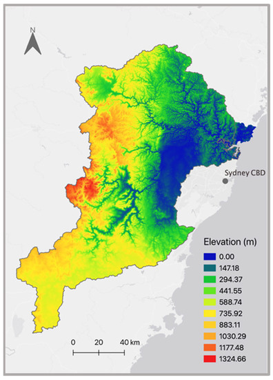
Figure 3.
Map of elevation in the Hawkesbury-Nepean Catchment before standardising with Fuzzy membership. Elevation is measured as metres above sea level.
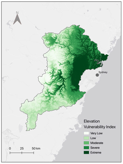
Figure 4.
Map of elevation Vulnerability in the Hawkesbury-Nepean Catchment after standardising with Fuzzy membership. Lighter colours indicate very low and low Vulnerability, while darker colours represent severe and extreme Vulnerability in accordance with Table 4.
3.2. Degree of Slope
Maps depicting degree of slope across the HNC before and after standardising with Fuzzy membership are presented in Figure 5 and Figure 6, respectively.
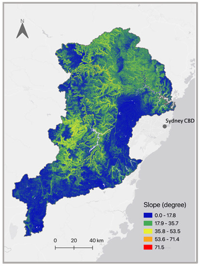
Figure 5.
Map depicting degree of slope across the Hawkesbury-Nepean Catchment before standardising with Fuzzy membership.
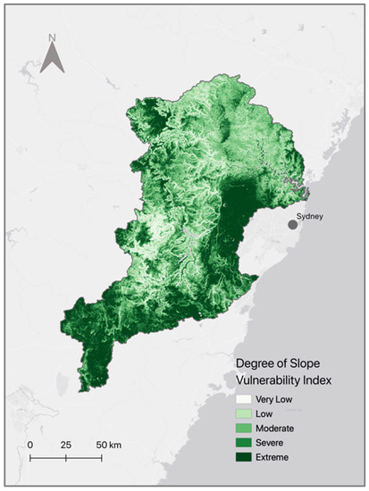
Figure 6.
Map depicting degree of slope Vulnerability across the Hawkesbury-Nepean Catchment after standardising with Fuzzy membership.
Figure 5 depicts the degree of slope data before standardising using Fuzzy Membership. Blue colour indicates the lowest degree of slope (0.0–17.8) which is prevalent in the HN Valley floodplain region as well as the southern part of the catchment. The highest degrees of slope can be seen in sparse areas in the Blue Mountains/Wollemi region in the west of the map (71.5). In the conservation areas in the western and north-western parts of the map, a moderate to high degree of slope is recorded (17.9–35.8). This trend is translated into the degree of slope index in Figure 6. Here, it can be seen that the highest slope vulnerability is located in the floodplain region of the valley. The lowest slope vulnerability (0.00–0.05) is depicted in the west and north-western area of the map, in the conservation regions of the catchment. Moderate slope vulnerability (0.06–0.38) is intertwined throughout the centre and western areas of the map.
3.3. IRSD
Maps depicting raw Index of Relative Socio-economic Disadvantage (IRSD) data across the HNC before and after standardising with Fuzzy membership are presented in Figure 7 and Figure 8, respectively.
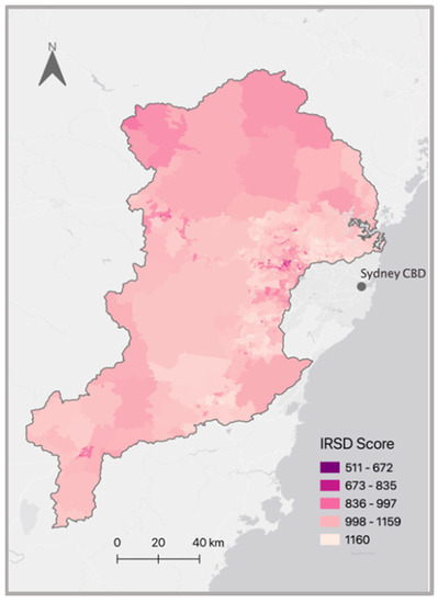
Figure 7.
Map depicting Index of Relative Socio-economic Disadvantage (IRSD) data across the Hawkesbury-Nepean Catchment before standardising with Fuzzy membership.
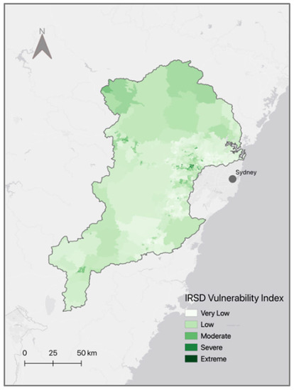
Figure 8.
Map depicting Index of Relative Socio-economic Disadvantage (IRSD) data across the Hawkesbury-Nepean Catchment after standardising with Fuzzy membership.
The raw IRSD data in Figure 7 was created using the methodology outlined in Section 2.6. Here, large gaps of data have been filled with an LGA average IRSD score. This has resulted in most of the conservation areas exhibiting a score range of approximately 998–1159. Low IRSD scores are also seen in the uppermost, western side of the map in the Lithgow City Council LGA (836–997). The lowest IRSD scores are found in SA2s in the GWS outer suburbs area that lies on the HN floodplain. Here, the lowest scores are recorded to be 511–672. Closer to the Sydney CBD and further towards the Ku-Ring-Gai, Northern Beaches, and The Shire of Hornsby, IRSD values become higher (1159–1160, the highest being 1160). The general trend shows a gradual decrease in IRSD score from the east to west. This trend is also apparent in the standardised map (Figure 8), where the north-western area of the map shows moderate vulnerability.
The magnified region in Figure 9 reveals the small SA2s that exhibit the cluster with the highest IRSD vulnerability in the catchment. These areas are located on the HN floodplain in the Liverpool, Penrith and Blacktown LGAs. The magnified map demonstrates the highest vulnerability level of some of these SA2s is extreme (0.94–1.00), with areas around this cluster displaying a severe vulnerability level (0.76–0.93). It can also be seen that the areas that show the lowest vulnerability (0.22–0.39) are situated around Ku-Ring-Gai, the Northern Beaches, and The Shire of Hornsby. A small, outlying group can be seen in the Goulburn region which is located at the southern point of the map. This group of SA2s shows moderate–severe vulnerability, which is unique from the higher values in the surrounding area.
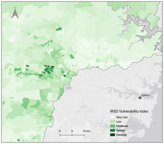
Figure 9.
Magnified map depicting Index of Relative Socio-economic Disadvantage (IRSD) data across GWS after standardising with Fuzzy membership. Including a map of the area of concern.
3.4. Hydrologic Soil Groups
Maps depicting raw Hydrologic Soil Group (HSG) data across the Hawkesbury-Nepean Catchment before and after standardising with Fuzzy membership are presented in Figure 10 and Figure 11, respectively.
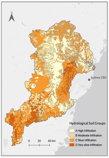
Figure 10.
Map depicting raw Hydrologic Soil Group (HSG) data across the Hawkesbury-Nepean Catchment before standardising with Fuzzy membership.
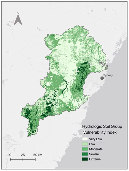
Figure 11.
Map depicting Hydrologic Soil Group (HSG) vulnerability across the Hawkesbury-Nepean Catchment after standardising with Fuzzy membership.
Raw HSG data is visualised in Figure 10 as a vector layer expressing the four classes according to their infiltration behaviour. These four classes are in accordance with those in Table 1. Figure 10 illustrates that the eastern floodplain region of the map is dominated by soils of hydrologic classes C and D and that this area is composed majorly of slow and very slow infiltration soils. These classes of soil are also littered around the northernmost part of the catchment, and are heavily present in the southern region as well. This southern part, especially the upper Lachlan Hills shire, the Goulburn Mulwaree council, and the Wingecarribee Shire are dominated by HSGs C and D. Soils with higher infiltration rates, (classes A and B) were found to be largely located in the Blue Mountains and Lithgow council areas (conservation areas).
Figure 11 displays the standardised data as a HSG vulnerability index. It indicates that the areas situated both in the HN Valley floodplain region and the southern area of the map contain the most clusters of extreme vulnerability. High vulnerability is attributed to low infiltration rates, with Figure 11 following the same trends depicted in Figure 10. The Blue Mountains region and the northern side of the map are mostly composed of very low–low vulnerability HSGs. The data was standardised using the automatic midpoint given by the ArcGIS Fuzzy Membership (small) tool, and this gave an even spread across the map. There were a few minor areas where water bodies were generalised as HSG class A. This meant that these lakes, rivers or creeks were automatically assigned the Vulnerability level of extreme. These areas were very small in comparison to the rest of the catchment area, and would not have to be addressed as it would not influence the final FVI.
3.5. Flood Vulnerability Index
The final Flood Vulnerability Index in the HNC as a combination of four indicators (Elevation, Slope, IRSD and Hydrologic Soil Groups) is presented in Figure 12.
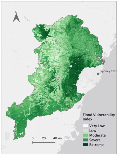
Figure 12.
Final Flood Vulnerability Index as a combination of four indicators (Elevation, Slope, IRSD and Hydrologic Soil Groups). This depicts the overall flood vulnerability in the Hawkesbury-Nepean catchment, with darker colours indicating higher vulnerability, and lighter colours indicating less vulnerability.
Figure 12 depicts the overall flood vulnerability index as a product of elevation, degree of slope, IRSD, and Hydrologic Soil Group vulnerability. The map uses the same green colour ramp as the previous standardised indicators, as well as the classification system from Table 4 to characterise FV. The map indicates the highest levels of FV in the GWS floodplain region, where severe to extreme levels of vulnerability are present. Severe and extreme levels are also found in the upper west of the study area. Very low to low FV is found to be in the western and northern regions of the map, with the lowest FV situated in the Lithgow City Council region. The southern and north eastern regions of the catchment were characterised by moderate/severe FV. The most vulnerable SA2s within the catchment are highlighted in Appendix B (Table A1).
Correlation analysis between each standardised indicator and the final FVI was conducted. It was found that elevation had the highest correlation value of 0.88. Secondary to this was slope, with a correlation value of 0.11, followed by IRSD (0.10), and then HSG (0.06). All indicators were positively and statistically significantly (p < 0.0001) correlated to the FVI.
4. Discussion
This study aimed to quantify FV through the use of an indicator-based multi-criteria analysis approach, and produce a FVI by considering indices which look at environmental vulnerability and societal vulnerability (elevation, slope, IRSD and HSG). Ultimately, the question driving this investigation asks whether or not an index based approach was useful in the assessment of FV, and how to best use the chosen indicators for this methodology. Additionally, this case study has endeavoured to provide actionable risk data. The following sections will discuss findings and the reasoning behind them.
4.1. Elevation
The raw data map created for elevation gives a comprehensive overview of the main topographic features of the HNC. From this map (Figure 3), it can be seen that the lowest values are mainly in the GWS region of the HN Valley. This region is an urbanised area encompassing the outer suburbs of Sydney, and contains both the Hawkesbury and Nepean rivers. It was expected that in areas closest to these main rivers, there will be low levels of elevation, and when compared to Figure 2 this was found to be evident. This was consistent with the fact that river beds are usually low lying due to running water eroding surrounding soil [47]. Places that lie closer to the coast were also expected to have lower elevation as they approach sea-level, and this is apparent in the north-eastern regions of Figure 3. The GWS area of the HN Valley is situated on a pre-existing flood plain, and is a long-established settlement since the 1800 s. Flood plains are formed by erosion removing sediment from either side of a river, creating a flat, low-lying area. Therefore, it is reasonable to assume that a flood plain will have a relatively low elevation in comparison to the land directly surrounding it, and this is reflected in Figure 3.
Other topographic characteristics that are demonstrated through this map are landforms. These landforms can be seen mainly in the middle to upper-western region of the catchment where a number of national parks are present. This area consists largely of the Blue Mountains, a region consisting of forested, mountainous land. The Blue Mountains and Wollemi areas are seen to have the highest elevation levels, with the exceptions of zones where main rivers are present. Sudden decline in elevation in the centre of the Blue Mountains region indicates a valley between two mountains. This is corroborated by the degree of slope outlined in Section 4.2.
Areas within a close distance to main rivers are identified as having severe–extreme vulnerability in Figure 4, and this is because moving waters in rivers act as an erosional agent that grinds down sediment to create low lying floodplains and valleys. When considering elevation closest to rivers and creeks it is important to note that these areas are at higher risk of fluvial flooding, where extreme precipitation can cause riverine overflows.
During pluvial flooding events, the highest elevation points on the index also experience less subsequent pooling from rain water, as they do not receive as much subsequent runoff from surrounding elevated areas. This is in contrast to the lowest areas which are susceptible to receiving watersheds from areas of higher elevation. This occurs particularly in valleys due to their characteristic U-shape cross section, or in floodplains that exhibit a ‘bowl’-like topography, where deluges of water have little opportunities for drainage. This topography can result in waters from extreme precipitation collecting in an area more readily and remaining in this area for longer.
In the topographically depressed areas of the HN valley, the low elevation combined with narrow sections in surrounding rivers creates what is called the ‘bathtub effect’. This effect is explored in a study by Munawar et al. (2022) [48]. There are several of these narrow sections found in rivers across the valley, these sections are called ‘choke points’ where large influxes of water are not able to be contained within the watercourse. Some of these choke points are located at Wallacia in the Warragamba River, Castlereagh in the Grose River, and Sackville in the Hawkesbury River. The low-lying conditions mean that the overflows caused by these choke points result in flood waters spreading quickly across a vast area. Munawar et al. [48] explains that it is this bathtub effect which has contributed to some of the most dangerous flood events in the HN catchment, and this is reflected by the elevation vulnerability index in Figure 4.
The initial midpoint set for this data during the Fuzzy Membership phase was the default value, which was the median point of the dataset. When first processed, this midpoint produced a map that was heavily skewed towards larger values, resulting in the standardised elevation map exhibiting majorly severe/extreme vulnerability. By consulting the raw elevation data in Figure 3 it was clear that this was not indicative of the true topographic vulnerability of the area, therefore an alternative midpoint was trialed. The mean value of the elevation dataset was instead utilised as the new midpoint which resulted in a more even distribution that highlighted the characteristics of the catchment more precisely.
The high correlation between elevation and the final FV map (0.92) is supported by the literature, as this indicator has been found to be largely influential in previous flood risk assessments [49,50].
4.2. Degree of Slope
The two maps in Figure 5 and Figure 6 depict both the raw and standardised versions of slope data for the HNC. Slope is distinct from elevation as it measures the steepness or angle of land instead of the relative height of the land. Similar to elevation, slope acts as an indicator for the physical morphology of the landscape, and expresses topographic elements that dictate the movement of water. For example, slope will indicate components such as ridge lines, plateaus, cliff faces, or gullies, which compound or mitigate vulnerability risk that cannot be determined with elevation data alone. This is why both elevation and slope complement each other to form a coherent picture of the HN catchment’s topography. These aforementioned components each have positive or negative consequences upon communities in HN’s flood prone areas.
Figure 5 depicts the north-western area of the catchment with the highest degrees of slope, with some of the highest values scattered around more remote national parks areas. This is expected as these areas are largely mountainous national and state park areas with varying undulation and landforms. This protected area has been exposed to significantly less development and land clearing, leaving many of these organic formations intact. These regions show low levels of flood vulnerability due to the fact that watersheds in these areas do not stay stagnant or pool. Instead, runoff is expected to leave the area quickly, meaning it has less potential to cause inundation.
Surface runoff generally moves at higher speeds in areas where higher degrees of slope are present, which heightens peak flow [51]. When areas such as these lie close to those of low elevation and slope, these low-lying areas are vulnerable to receiving this high velocity watershed. This is particularly relevant in pluvial flooding scenarios. In the instance of the HNC, the location of communities is in the low lying HN Valley, situated in GWS. From Figure 6, it can be seen that as a result of the preceding conditions in the protected, elevated areas, the HN Valley area shows extreme vulnerability to high levels of runoff, potentially resulting in flash flooding. These extreme levels are also seen in the uppermost-western region of the map and also in the south of the catchment, as these areas are considered relatively flat in comparison to the mountainous regions mentioned previously. From this reasoning, it was expected that low lying land positioned at the foot of slopes with high runoff potential would exhibit the highest vulnerability in the catchment area, as this is aligned with common findings in previous research such as Ajmal et al. (2020) [52]. From Figure 6, these areas are in fact highlighted as having extreme vulnerability, however they are difficult to visualise in the presence of other extreme areas on the map. The values for degree of slope show some acute changes when surpassing the midpoint, with the majority of the HN valley depicted as extremely vulnerable. In Figure 5, the large blue area does not show the variation between areas at the foot of high slope areas and the low-lying floodplain. This was due to the midpoint selection of the data.
The midpoint of the slope data was manually changed from the default value to the mean of the data similar to that of elevation. This was because it presented more evenly distributed data. Once changed, the map produced was able to give potential stakeholders a comprehensive view of the variability of the catchment for actionable data usage. This midpoint could have been further investigated in order to reveal the variation between areas next to high slope, and low-lying areas at a distance from higher slope.
While a number of flat areas exhibited high vulnerability (particularly in the southern part of the catchment), combining the results with elevation data in the final FVI established the true manifestation of the effects of slope. This is because elevation data in Figure 3 and Figure 4 illustrate that the southern localities in the catchment reveal moderate elevation and thus low vulnerability levels. In contrast, the areas with relatively higher degrees of slope experience lower vulnerability. The combination of moderate to high elevation and low degrees of slope indicates that an area is a high-lying plateau rather than a low flood plain. In this case, these areas would not be exceedingly susceptible to flood events as they are not made vulnerable by the bathtub effect outlined in Section 4.1. While there are a number of rivers present in the southern part of the catchment, the lack of deep floodplain topography would result in lower vulnerability overall.
Areas of extreme slope vulnerability in Figure 6, such as the HN Valley floodplain region, are at a high risk of waterlogging. As a result of a broad lack of avenues for accumulating rainfall to escape from the region, this low-lying flat area has the potential to see severe inundation of water from extreme precipitation events. As heavy rainfall accumulates there is very little topographic drainage present in the area to divert the flow of water elsewhere. The build-up of precipitation in this one area can saturate the soil below, meaning the residual water will remain on the surface. This can take hours to even weeks to subside, alluding to elevated flood risk during these periods. This connection to soil and its water holding capacity is further discussed in Section 4.4.
We found that slope had a much weaker positive correlation value when compared with the overall FV map (0.17). On a surface level, the appearance of the final index seems to be visually similar to that of the slope index. However, once processed in Python this was found to be misleading. The numerical extremes seen in this data may offer a reason as to why this low correlation has occurred. These extremes are seen in Figure 6 where there is a large jump from moderate vulnerability (0.38) to severe vulnerability (0.96). This distribution is not as evenly spaced as the elevation data. The extremely high resolution of this data (1 s or 30 m) seen in Table 2 could also be a reason as to why this layer did not correlate highly with the overall index, as it was much more detailed than any other layer.
The nature of human settlement in the HNC means that urbanised areas are subject to the physical vulnerabilities posed by low-lying flat areas. It is intuitive that historically humans generally tend to settle and build civilisations around water bodies, and that flat, cleared areas have been favoured for this [28]. This is also true for the establishment of farms. However, the progression of understanding flood hazards and their increase in frequency over time indicates that these settlements are made extremely vulnerable for these very same reasons.
4.3. Index of Relative Socio-Economic Disadvantage
The IRSD data gave an insight into where the socio-economic factors of the HNC influence vulnerability the most, as well as how these factors spatially compare to the physical environment.
The areas of the IRSD map that were initially ‘no data zones’ discussed in Section 2.6 exhibited a very-low to low vulnerability level after standardising. This was expected due to the attributes of the state and national parks areas as well as industrial, non-residential areas. However, especially in the state and national parks with no permanent population, it was initially expected that these areas would have even lower vulnerability than what was presented in Figure 8. This is because it would be expected to see less vulnerability in an area that has no exposed population. Other methods could have been trialled to ensure that this data was more precise.
The IRSD vulnerability index had a relatively low correlation to the overall FV index in comparison to elevation (0.10). This very weak positive correlation might be related to the layer having the lowest resolution of data, as well as significant data gaps that required manual cleaning. While there was a cluster of extreme values, the dominant class of vulnerability for the study area was 0.22–0.57 (Very low–Low). Therefore, when compared to all environmental indicator maps, the overall value does not correlate highly. This is also exhibited by many rural areas having more moderate levels of vulnerability, whereas all physical indicators showed these areas as the least vulnerable. On a macroscale, it can be deduced that IRSD may not play a large role in the vulnerability of the broader catchment. However, on a smaller community level, critical local vulnerabilities should be carefully considered.
Low IRSD (higher vulnerability) is expected in communities with less access to infrastructure. This trend is generally seen in rural areas that are less developed as a result of their isolated locations and distance from main cities and towns [53]. Therefore, some of the higher results for indicators that constitute the IRSD such as ‘employed people classified as low skill Community and Personal Service workers’ or ‘people aged 15 years and over who have no educational attainment’ can be expected in more isolated areas.
The most urbanised communities in NSW tend to neighbour the coastline, which is true for many populations in Australia. NSW’s capital city Sydney, lies in this vicinity, and due to its ever-developing nature it has grown to encompass a large area of the HN Valley as its outer suburbs. It was expected that SA2s located closer to the inner-city, or Sydney CBD will exhibit higher IRSD scores (lower vulnerability) due to well established localities and access to infrastructure. This was supported by the IRSD map (Figure 7) which indicates lighter colours around the northern beaches and closer to Sydney CBD, and generally, darker shades moving further into regional NSW.
This trend saw a number of outliers as some of the lowest IRSD values in the catchment were recorded in the GWS region. These areas were found to be in Blacktown, Penrith, Liverpool, Hawkesbury, and Fairfield. While the IRSD in these areas was relatively low in comparison to surrounding localities, it is also important to note that those areas such as Penrith are only ranked in the 44th percentile in Australia according to the SEIFA index. This means that while some neighbouring areas in the Hills Shire show very low levels of relative disadvantage, there are still extremely vulnerable communities situated close by. Due to the vulnerability highlighted in this area (Figure 8), it could be assumed that flood risk is an implicit factor in this low IRSD score. Further investigation into this area reveals that government housing is present in a number of areas corresponding to these low IRSD scores in Fairfield, Blacktown, and Liverpool. IRSD indicators such as ‘occupied private dwellings paying rent less than $215 per week’ and low incomes (see Appendix A) can be indicative of areas containing government housing. Additionally, the fact that these disadvantaged communities are specifically located within the low-lying flood plain area make them of greater concern in comparison to low IRSD levels outside of the flood plain. This nature of the outer suburbs exhibits how disadvantages can manifest in places of urban sprawl [54]. A 2015 report by the Australian Housing and Urban Research Institute found that susceptibility to natural hazards is an additional factor contributing to affordable housing and subsequent disadvantage in an area [55]. This has caused a feedback loop in which housing costs become lower in areas of high FV, attracting buyers who may not be able to afford insurance associated with living in a high flood risk area. This can see disadvantaged communities being less likely to recover from a flood event.
Urbanisation on floodplains has ultimately resulted in the exposure of communities to flood hazards, and the impacts felt by these communities are lessened or heightened by their socioeconomic vulnerability. Ultimately, continuing to expand communities in this low-lying, vulnerable area is not sustainable, especially with extreme precipitation events in the HNC becoming more frequent and severe. This coupled with a growing population could see more disadvantaged individuals being left vulnerable in the face of extreme pluvial and fluvial flood events.
4.4. Hydrologic Soil Groups
HSG was found to follow a similar spatial pattern to elevation and slope, and also highlighted the vulnerability of the floodplain in Figure 10 and Figure 11. HSGs are dictated by the composition and structure of the topsoil in a given location. Historically, the groups A, B, C, and D have been assigned in accordance with these soil characteristics. Soil type A or high infiltration soils consist of larger pore spaces, larger soil aggregates and larger amounts of sand and organic matter in their compositions. This increased spacing within the topsoil creates deposits that readily accept surface water. The ability for these soils to absorb this water means that there tends to be less runoff and therefore less chance of fast-moving flood waters causing devastation in areas that consist of them.
Historically, the capacity for this soil to allow infiltration is measured in hydraulic conductivity [56] a quantitative measure of a saturated soil’s ability to transmit water when subjected to a hydraulic gradient. High infiltration soils (type A) have a saturated hydraulic conductivity of 40 micrometres per second. In contrast, type D soils consist largely of clay and silt, which have significantly smaller particle sizes than that of sand. The saturated hydraulic conductivity of type D soils is generally 1.0 micrometres per second. These soils contain smaller pore spaces between soil aggregates, leaving less room for infiltration. These soils are expected to absorb less water, resulting in runoff remaining on the surface with nowhere to discharge. This is also heightened when external forces compact the soil, squashing pore spaces within the ground and allowing for less infiltration.
Figure 10 indicates that group A soils are mainly situated in protected, forested areas, particularly in the Blue Mountains region. The largely undisturbed nature of the soils in these areas means that very little compaction has occurred from anthropogenic interventions. This allows the earth in this area to maintain pore space [57]. The increased organic matter within this location due to dense vegetation also contributes to decreased runoff potential of the soil. The forested areas consist of significantly more biomass than urbanised or cleared areas. This biomass enters the ground either through root systems or organic litter, assisting in the aggregation of the soil and increasing pore space [58]. This vegetation also has the potential to protect the soil beneath it from erosion, meaning that it will maintain the soil structure, as well as the degree of topographic relief. The presence of type A soils in this area of high slope means that soils will have more water absorbing characteristics while slope will encourage faster runoff. Further investigation has determined that the degree of slope will have a dominant impact on the behaviour of runoff in comparison to HSG.
Conversely, areas that have had more anthropogenic interference will be more compacted, and consist of less organic matter. Many soils in urban areas are labelled ‘Anthroposols’ as they have been tampered with so much that their original composition is permanently changed. These urban soils tend to be more silt/clay heavy, and obstruct infiltration [57]. A lack of vegetation in these areas also means that the soils are exposed to erosion, which breaks soil aggregates, resulting in smaller soil particles which allow less pore space between them. Figure 10 illustrated this link, whereby the most urbanised areas on the HN flood plain consist of class C and D soils. It is these areas that express the highest vulnerability in the resulting HSG index (Figure 11). This low infiltration behaviour is also enhanced by anthropogenic materials found in urban areas (e.g., asphalt, concrete, metals, etc.). These materials combined with type C and D soils have the potential to contribute to high velocity flash flood events. Around water bodies this low infiltration behaviour can allow overflows to travel widely.
HSG showed the lowest correlation to the overall FVI (0.04). This low correlation could be due to the fact that the HSG data was categorical, and only varied between four soil categories. In contrast, other indicators had numerous data points separated into natural breaks. The difference in the nature of the HSG data may have impacted how this layer related to the others.
4.5. Flood Vulnerability Index
After combining all four indicator indices using the Fuzzy Gamma Overlay tool, the resulting map showed a successful, high-resolution depiction of the FVI over the HN catchment (Figure 12). The most noticeable trend emphasises the GWS communities on the HN Valley flood plain as extremely vulnerable, with the central-western region exhibiting the lowest levels of vulnerability. This is a culmination of the conclusions drawn from Section 4.1, Section 4.2, Section 4.3 and Section 4.4.
Outlying regions include the uppermost-western part of the map identified as a part of Lithgow. This region was labelled with severe–extreme vulnerability in all indicator maps. However, while this area exhibits low elevation, slope, and IRSD along with slow infiltration soils, it has not historically been subjected to high hazard vulnerability, however a changing climate may affect this. Future collaboration between hazard and vulnerability studies has the potential to reveal this relationship. The past instances of extreme flood have been in the flood plain region of the catchment, making this area of higher interest than the Lithgow area. Regions in the south of the map show moderate–severe FV, mostly due to slope and HSG data.
Each of the indicators used to produce the final FVI provide concise information regarding the characteristics of the catchment. However, alone each indicator has a level of ambiguity. It is with the combination of all four indicators that the relationships between this data comes to light, and the interplay between the physical and socio-economic characteristics becomes apparent. For example, when viewed in isolation, the degree of slope can mislead viewers into thinking that all flat land is highly vulnerable. When combined with elevation it is noticed that high, flat areas are less susceptible to flooding. Another relationship can be drawn between elevation, slope, and HSG, where high infiltration soils generally occur in the higher, undisturbed conservation regions. HSG alone informs the viewer that high infiltration soil in the Blue Mountains region of the catchment will lead to less runoff, however, when looked at in combination with slope data, it was found that slope would also contribute highly to the behaviour of watersheds, and the magnitude of each of these indicators’ influence is difficult to decipher. Finally, IRSD and the distribution of human populations can be related to slope and elevation, as historically colonial settlements tend to occur in flat areas close to water bodies.
5. Conclusions
With flood prone Australian communities likely to experience more intense and frequent extreme flood hazards in the future, it is important to assess their physical and socio-economic vulnerabilities to better understand what may turn these flood hazards into disasters. This study was centralised around this concept, and aimed to create a flood vulnerability index for the Hawkesbury-Nepean catchment from relevant, compatible and readily accessible indicators. The topographic morphology of the region was explored through elevation and degree of slope indicators in order to express how the movement of flood waters can be heightened. These indicators were compared to the hydrologic soil group indicator, which assessed how the composition of soils can also be an influential physical factor. Finally, the socio-economic characteristics of the catchment were represented by the index of relative socio-economic disadvantage, which revealed the ability for people to cope and adapt. These indicators were combined to produce an overall flood vulnerability index of the study area.
Flood vulnerability was shown to be at its highest in the Hawkesbury-Nepean valley flood plain region on the outskirts of Greater Western Sydney. Here, the highest values were recorded in Blacktown, Penrith, and Liverpool, with the most extreme value (0.95) being recorded in the Bidwill-Herbersham-Emerton SA2 region (Blacktown). It was found that a combination of low elevation, low degree of slope, low IRSD score, and very-low infiltration soils resulted in very high levels of vulnerability. Therefore, the low lying, flat, highly urbanised area of the HN floodplain was evidently the most vulnerable area in the catchment. Combining all four indicators into a standardised flood vulnerability index clearly showed a more substantial view of vulnerability than any individual indicator alone.
This study will act as the foundation for further assessment of the overall flood risk of the catchment combining the vulnerability index with both hazard and exposure indices. This intends to give the actionable risk data from this study the ability to reach relevant stakeholders who wish to adopt index-based approaches within flood prone regions. The fact that this novel approach is replicable for the whole country makes it easily accessible to those who have a vested interest in flood risk mitigation and adaptation. Before this, there is great opportunity for elaboration on flood vulnerability and improvement to this proof-of-concept methodology.
This inquiry into the flood vulnerability of the Hawkesbury-Nepean catchment ultimately highlights environmental and socio-economic index techniques that are somewhat overlooked. It also brings to light the fact that the flood hazard itself can be largely influenced by the environment around it. By viewing natural disasters as being influenced by vulnerability factors, those decision makers and stakeholders can feel more empowered to make proactive, risk informed decisions. This is because many of these vulnerability factors have the ability to be addressed, whereas the occurrence of the flood itself may be out of human control. In the future, addressing vulnerability in FRAs will enhance the proactive management of flood disasters, and ultimately build greater flood resilience.
Author Contributions
Conceptualization, I.S. and Y.K.; methodology, I.S. and Y.K.; software, I.S.; validation, I.S.; formal analysis, I.S.; investigation, I.S.; resources, Y.K.; data curation, I.S.; writing—original draft preparation, I.S.; writing—review and editing, I.S. and Y.K.; visualization, I.S.; supervision, Y.K.; project administration, Y.K.; funding acquisition, Y.K. All authors have read and agreed to the published version of the manuscript.
Funding
This research received no external funding.
Data Availability Statement
Not applicable.
Acknowledgments
Authors express sincere gratitude to colleagues from the Climate Risk and Early Warning Systems (CREWS) team at the Australian Bureau of Meteorology and Monash University for their helpful advice and guidance.
Conflicts of Interest
The authors declare no conflict of interest.
Appendix A
A detailed list of all the indicators used in the IRSD index provided by the ABS.
The variables used in the index are listed below. All variables in this index are indicators of disadvantage. INC_LOW is the strongest indicator of disadvantage (ABS 2018).
- INC_LOW: % of people with stated household equivalised income between $1 and $25,999 per year
- CHILDJOBLESS: % of families with children under 15 years of age who live with jobless parents
- NONET: % of occupied private dwellings with no internet connection
- NOYEAR12ORHIGHER: % of people aged 15 years and over whose highest level of education is Year 11 or lower
- UNEMPLOYED: % of people (in the labour force) who are unemployed
- OCC_LABOUR: % of employed people classified as Labourers
Appendix B
Table A1.
Summary of the most vulnerable communities within the Hawkesbury-Nepean catchment by statistical area 2.
Table A1.
Summary of the most vulnerable communities within the Hawkesbury-Nepean catchment by statistical area 2.
| SA 2 | LGA | Flood Vulnerability Score | Flood Vulnerability Risk Class |
|---|---|---|---|
| Bidwill-Herbersham-Emerton | Blacktown City Council | 0.95 | Extreme |
| Whalan | Blacktown City Council | 0.93 | Severe |
| Lethbridge Park—Tregear | Blacktown City Council | 0.93 | Severe |
| Colyton—Oxley Park | Penrith City Council | 0.92 | Severe |
| Badgerys Creek | Liverpool City Council | 0.92 | Severe |
References
- Wasko, C.; Nathan, R.; Stein, L.; O’Shea, D. Evidence of Shorter More Extreme Rainfalls and Increased Flood Variability under Climate Change. J. Hydrol. 2021, 603, 126994. [Google Scholar] [CrossRef]
- Australian Bureau of Meteorology (BoM). Understanding Floods; Australian Government Bureau of Meteorology. Available online: http://www.bom.gov.au/australia/flood/knowledge-centre/understanding.shtml (accessed on 4 May 2022).
- Sarkar, D.; Saha, S.; Mondal, P. GIS-Based Frequency Ratio and Shannon’s Entropy Techniques for Flood Vulnerability Assessment in Patna District, Central Bihar, India. Int. J. Environ. Sci. Technol. 2022, 19, 8911–8932. [Google Scholar] [CrossRef]
- Suchara, I. The Impact of Floods on the Structure and Functional Processes of Floodplain Ecosystems. JSPB 2019, 1, 44–60. [Google Scholar] [CrossRef]
- Monk, W.A.; Compson, Z.G.; Choung, C.B.; Korbel, K.L.; Rideout, N.K.; Baird, D.J. Urbanisation of Floodplain Ecosystems: Weight-of-Evidence and Network Meta-Analysis Elucidate Multiple Stressor Pathways. Sci. Total Environ. 2019, 684, 741–752. [Google Scholar] [CrossRef]
- Zhi, G.; Liao, Z.; Tian, W.; Wu, J. Urban Flood Risk Assessment and Analysis with a 3D Visualization Method Coupling the PP-PSO Algorithm and Building Data. J. Environ. Manag. 2020, 268, 110521. [Google Scholar] [CrossRef]
- Database | EM-DAT. Available online: https://www.emdat.be/database (accessed on 26 May 2022).
- Rahman, A.; Charron, C.; Ouarda, T.B.M.J.; Chebana, F. Development of Regional Flood Frequency Analysis Techniques Using Generalized Additive Models for Australia. Stoch. Environ. Res. Risk Assess. 2018, 32, 123–139. [Google Scholar] [CrossRef]
- Insurance Council of Australia (ICA). Climate Change Impact Series: Flooding and Future Risks; Insurance Council of Australia (ICA): Sydney, NSW, Australia, 2022. [Google Scholar]
- Bates, P.D.; Quinn, N.; Sampson, C.; Smith, A.; Wing, O.; Sosa, J.; Savage, J.; Olcese, G.; Neal, J.; Schumann, G.; et al. Combined Modeling of US Fluvial, Pluvial, and Coastal Flood Hazard Under Current and Future Climates. Water Resour. Res. 2021, 57, e2020WR028673. [Google Scholar] [CrossRef]
- Holgate, C.; Evans, J.P.; Taschetto, A.S.; Gupta, A.S.; Santoso, A. The Impact of Interacting Climate Modes on East Australian Precipitation Moisture Sources. J. Clim. 2022, 35, 3147–3159. [Google Scholar] [CrossRef]
- Tabari, H. Climate Change Impact on Flood and Extreme Precipitation Increases with Water Availability. Sci. Rep. 2020, 10, 13768. [Google Scholar] [CrossRef]
- Ishak, E.; Rahman, A. Examination of Changes in Flood Data in Australia. Water 2019, 11, 1734. [Google Scholar] [CrossRef]
- Intergovernmental Panel on Climate Change (IPCC). Summary for Policymakers. In Climate Change 2022: Impacts, Adaptation and Vulnerability: Contribution of Working Group II to the Sixth Assessment Report of the Intergovernmental Panel on Climate Change; Cambridge University Press: Cambridge, UK, 2022. [Google Scholar]
- Crichton, D. The Risk Triangle. In Natural Disaster Management; Tudor Rose: London, UK, 1999; pp. 102–103. Available online: https://www.ilankelman.org/crichton/1999risktriangle.pdf (accessed on 1 August 2022).
- McGregor, J.; Parsons, M.; Glavac, S. Local Government Capacity and Land Use Planning for Natural Hazards: A Comparative Evaluation of Australian Local Government Areas. Plan. Pract. Res. 2022, 37, 248–268. [Google Scholar] [CrossRef]
- Ferreira, T.; Santos, P. An Integrated Approach for Assessing Flood Risk in Historic City Centres. Water 2020, 12, 1648. [Google Scholar] [CrossRef]
- Ologunorisa, T.E.; Abawua, M.J. Flood Risk Assessment: A Review. J. Appl. Sci. Environ. Manag. 2005, 9, 57–63. [Google Scholar]
- Merz, B.; Aerts, J.; Arnbjerg-Nielsen, K.; Baldi, M.; Becker, A.; Bichet, A.; Blöschl, G.; Bouwer, L.M.; Brauer, A.; Cioffi, F.; et al. Floods and Climate: Emerging Perspectives for Flood Risk Assessment and Management. Nat. Hazards Earth Syst. Sci. 2014, 14, 1921–1942. [Google Scholar] [CrossRef]
- Australian Institute of Disaster Resilience (AIDR). Managing the Floodplain: A Guide to Best Practice in Flood Risk Management in Australia. In Australian Disaster Resilience Handbook Collection: Handbook 7; Australian Institute of Disaster Resilience (AIDR): Melbourne, VIC, Australia, 2017. [Google Scholar]
- De Brito, M.M.; Evers, M. Multi-Criteria Decision-Making for Flood Risk Management: A Survey of the Current State of the Art. Nat. Hazards Earth Syst. Sci. 2016, 16, 1019–1033. [Google Scholar] [CrossRef]
- Batica, J.; Gourbesville, P. From Catstrophe to Resilience; Springer Nature Switzerland: Cham, Switzerland, 2020; pp. 121–133. ISBN 978-9-81155-435-3. [Google Scholar]
- Deepak, S.; Rajan, G.; Jairaj, P.G. Geospatial Approach for Assessment of Vulnerability to Flood in Local Self Governments. Geoenviron. Disasters 2020, 7, 35. [Google Scholar] [CrossRef]
- Ntajal, J.; Lamptey, B.; Mianikposogbedji, J. Flood Vulnerability Mapping in the Lower Mono River Basin in Togo, West Africa. Int. J. Sci. Eng. Res. 2016, 7, 1553–1562. [Google Scholar]
- Chen, Y.; Ye, Z.; Liu, H.; Chen, R.; Liu, Z.; Liu, H. A GIS-Based Approach for Flood Risk Zoning by Combining Social Vulnerability and Flood Susceptibility: A Case Study of Nanjing, China. Int. J. Environ. Res. Public Health 2021, 18, 11597. [Google Scholar] [CrossRef]
- Coates, J. Draft Floodplain Risk Management Study and Plan Report. 2017. Available online: https://www.hawkesbury.nsw.gov.au/__data/assets/pdf_file/0017/52820/ORD_DEC_2012_Att1toItem224V1.pdf (accessed on 1 August 2022).
- Smith, E.F.; Keys, N.; Lieske, S.N.; Smith, T.F. Assessing Socio-Economic Vulnerability to Climate Change Impacts and Environmental Hazards in New South Wales and Queensland, Australia. Geogr. Res. 2015, 53, 451–465. [Google Scholar] [CrossRef]
- Nasiri, H.; Mohd Yusof, M.J.; Mohammad Ali, T.A. An Overview to Flood Vulnerability Assessment Methods. Sustain. Water Resour. Manag. 2016, 2, 331–336. [Google Scholar] [CrossRef]
- Micevski, T.; Franks, S.W.; Kuczera, G. Multidecadal Variability in Coastal Eastern Australian Flood Data. J. Hydrol. 2006, 327, 219–225. [Google Scholar] [CrossRef]
- Gillespie, C.; Grech, P.; Bewsher, D. Reconciling Development with Flood Risks: The Hawkesbury-Nepean Dilemma. Aust. J. Emerg. Manag. 2022, 17, 27–32. [Google Scholar] [CrossRef]
- Alaoui, A.; Rogger, M.; Peth, S.; Blöschl, G. Does Soil Compaction Increase Floods? A Review. J. Hydrol. 2018, 557, 631–642. [Google Scholar] [CrossRef]
- Fereshtehpour, M.; Karamouz, M. DEM Resolution Effects on Coastal Flood Vulnerability Assessment: Deterministic and Probabilistic Approach. Water Resour. Res. 2018, 54, 4965–4982. [Google Scholar] [CrossRef]
- Warren, S.D.; Hohmann, M.G.; Auerswald, K.; Mitasova, H. An Evaluation of Methods to Determine Slope Using Digital Elevation Data. CATENA 2004, 58, 215–233. [Google Scholar] [CrossRef]
- Meraj, G.; Romshoo, S.A.; Yousuf, A.R.; Altaf, S.; Altaf, F. Assessing the Influence of Watershed Characteristics on the Flood Vulnerability of Jhelum Basin in Kashmir Himalaya. Nat. Hazards 2015, 77, 153–175. [Google Scholar] [CrossRef]
- Mahmoud, S.H.; Gan, T.Y. Multi-Criteria Approach to Develop Flood Susceptibility Maps in Arid Regions of Middle East. J. Clean. Prod. 2018, 196, 216–229. [Google Scholar] [CrossRef]
- Australian Bureau of Statistics (ABS). Socio-Economic Indexes for Areas (SEIFA); Australian Bureau of Statistics (ABS): Canberra, Australia, 2018.
- Jaffrés, J.B.D.; Cuff, B.; Cuff, C.; Faichney, I.; Knott, M.; Rasmussen, C. Hydrological Characteristics of Australia: Relationship between Surface Flow, Climate and Intrinsic Catchment Properties. J. Hydrol. 2021, 603, 126911. [Google Scholar] [CrossRef]
- Ross, C.W.; Prihodko, L.; Anchang, J.; Kumar, S.; Ji, W.; Hanan, N.P. HYSOGs250m, Global Gridded Hydrologic Soil Groups for Curve-Number-Based Runoff Modeling. Sci. Data 2018, 5, 180091. [Google Scholar] [CrossRef]
- Zeng, Z.; Tang, G.; Hong, Y.; Zeng, C.; Yang, Y. Development of an NRCS Curve Number Global Dataset Using the Latest Geospatial Remote Sensing Data for Worldwide Hydrologic Applications. Remote Sens. Lett. 2017, 8, 528–536. [Google Scholar] [CrossRef]
- Abdel-Fattah, M.; Kantoush, S.A.; Saber, M.; Sumi, T. Rainfall-Runoff Modeling for Extreme Flash Floods in Wadi Samail, Oman. J. Jpn. Soc. Civ. Eng. Ser. B1 (Hydraul. Eng.) 2018, 74, I_691–I_696. [Google Scholar] [CrossRef]
- Chen, H.; Zhang, X.; Abla, M.; Lü, D.; Yan, R.; Ren, Q.; Ren, Z.; Yang, Y.; Zhao, W.; Lin, P.; et al. Effects of Vegetation and Rainfall Types on Surface Runoff and Soil Erosion on Steep Slopes on the Loess Plateau, China. CATENA 2018, 170, 141–149. [Google Scholar] [CrossRef]
- Aitkenhead, I.; Kuleshov, Y.; Watkins, A.B.; Bhardwaj, J.; Asghari, A. Assessing Agricultural Drought Management Strategies in the Northern Murray–Darling Basin. Nat. Hazards 2021, 109, 1425–1455. [Google Scholar] [CrossRef] [PubMed]
- Do, C.; Kuleshov, Y. Multi-hazard Tropical Cyclone Risk Assessment for Australia. Nat. Hazards Earth Syst. Sci. Discuss. 2022. in review. [Google Scholar] [CrossRef]
- Dunne, A.; Kuleshov, Y. Drought Risk Assessment and Mapping for the Murray-Darling Basin, Australia. Nat. Hazards 2022. [Google Scholar] [CrossRef]
- AURIN Portal: AURIN. Australian Urban Research Infrastructure Network. Available online: https://aurin.org.au/resources/aurin-portal/ (accessed on 1 July 2022).
- Lyerly, S.B. The Average Spearman Rank Correlation Coefficient. Psychometrika 1952, 17, 421–428. [Google Scholar] [CrossRef]
- Lowe, M.-A.; McGrath, G.; Leopold, M. The Impact of Soil Water Repellency and Slope upon Runoff and Erosion. Soil Tillage Res. 2021, 205, 104756. [Google Scholar] [CrossRef]
- Munawar, H.S.; Mojtahedi, M.; Hammad, A.W.A.; Ostwald, M.J.; Waller, S.T. An AI/ML-Based Strategy for Disaster Response and Evacuation of Victims in Aged Care Facilities in the Hawkesbury-Nepean Valley: A Perspective. Buildings 2022, 12, 80. [Google Scholar] [CrossRef]
- Leitão, J.P.; de Sousa, L.M. Towards the Optimal Fusion of High-Resolution Digital Elevation Models for Detailed Urban Flood Assessment. J. Hydrol. 2018, 561, 651–661. [Google Scholar] [CrossRef]
- Ogania, J.L.; Puno, G.R.; Alivio, M.B.T.; Taylaran, J.M.G. Effect of Digital Elevation Model’s Resolution in Producing Flood Hazard Maps. Glob. J. Environ. Sci. Manag. 2019, 5, 95–106. [Google Scholar] [CrossRef]
- Adnan, M.S.G.; Dewan, A.; Zannat, K.E.; Abdullah, A.Y.M. The Use of Watershed Geomorphic Data in Flash Flood Susceptibility Zoning: A Case Study of the Karnaphuli and Sangu River Basins of Bangladesh. Nat. Hazards 2019, 99, 425–448. [Google Scholar] [CrossRef]
- Ajmal, M.; Waseem, M.; Kim, D.; Kim, T.-W. A Pragmatic Slope-Adjusted Curve Number Model to Reduce Uncertainty in Predicting Flood Runoff from Steep Watersheds. Water 2020, 12, 1469. [Google Scholar] [CrossRef]
- De Silva, M.M.G.T.; Kawasaki, A. Socioeconomic Vulnerability to Disaster Risk: A Case Study of Flood and Drought Impact in a Rural Sri Lankan Community. Ecol. Econ. 2018, 152, 131–140. [Google Scholar] [CrossRef]
- Wynne, L.; Ruoso, L.-E.; Cordell, D.; Jacobs, B. ‘Locationally Disadvantaged’: Planning Governmentalities and Peri-Urban Agricultural Futures. Aust. Geogr. 2020, 51, 377–397. [Google Scholar] [CrossRef]
- Miller, W. What Does Built Environment Research Have to Do with Risk Mitigation, Resilience and Disaster Recovery? Sustain. Cities Soc. 2015, 19, 91–97. [Google Scholar] [CrossRef]
- Werner, J.; Woodward, D.; Nielsen, R.; Dobos, R.; Hjelmfelt, A.; Hoeft, C.C. Hydrologic Soil Groups. In Part 630 Hydrology—National Engineering Handbook; USDA Natural Resource Conservation Service (NRCS): Washington, DC, USA, 2009; Chapter 7. [Google Scholar]
- Hou, X.; Jia, Z.; Han, Q.; Sun, H.; Wang, W.; Nie, J.; Yang, B. Effects of Different Rotational Tillage Patterns on Soil Structure, Infiltration and Water Storage Characteristics in Dryland. Trans. Chin. Soc. Agric. Eng. 2012, 28, 85–94. [Google Scholar]
- Auerswald, K.; Gu, Q.-L. Reassessment of the Hydrologic Soil Group for Runoff Modelling. Soil Tillage Res. 2021, 212, 105034. [Google Scholar] [CrossRef]


Publisher’s Note: MDPI stays neutral with regard to jurisdictional claims in published maps and institutional affiliations. |
© 2022 by the authors. Licensee MDPI, Basel, Switzerland. This article is an open access article distributed under the terms and conditions of the Creative Commons Attribution (CC BY) license (https://creativecommons.org/licenses/by/4.0/).