Unbiased Area Estimation Using Copernicus High Resolution Layers and Reference Data

Abstract

Land cover area estimates can be derived via design-based approaches using a probability (random) reference sample. The collection of samples is usually costly and requires an effective sampling design. Earth-Observation-based mapping approaches do not have this requirement but can be biased in providing area estimates. Combining reference samples with remote sensing products can reduce sampling efforts and provide a more effective method to estimate land cover. The Copernicus High-Resolution Layer (HRL) provides remote-sensing-based data across Europe to support area estimation. Different methods are tested to estimate areas of imperviousness in four selected countries in Europe to demonstrate the use and shortcomings of existing reference information from the LUCAS survey program and the HRL Imperviousness products from 2015 and 2018.

1. Introduction

Precise area estimates of land cover/land use (LCLU) are central for various management and monitoring strategies. Area can be estimated in either a design-based or model-based inference framework. In a design-based framework, population parameters such as the area of a certain land cover are estimated on the basis of a sample of reference observations. Despite the scientific progress, consensus and guidance from intergovernmental organisations, such as the Global Forest Observations Initiative’s “Methods and Guidance Documents” [1] or the United Nations Food and Agriculture Organisation’s “Global Strategy to improve Agricultural and Rural Statistics” [2], simplified approaches for area estimation and unquestioned uses of Earth Observation (EO) data acquired by remote sensing are still reported [3].

The increasing accessibility of EO data and services through the Copernicus program have stimulated the use of such data and products for monitoring and decision making. The Pan-European Copernicus High-Resolution Layers (HRL) [4] provide specific LCLU products, such as on sealed/impervious surfaces, forests, grasslands, or water bodies and wetness conditions. These products are based on satellite data, in particular the Copernicus Sentinel-1 and -2 sensors [4] and thus provide the potential to support area statistics [5].

The simplest approach to use EO-based LCLU maps for area estimation is by summing the area covered by the classified remote sensing pixels (i.e., the number of pixels per class times the area size of a pixel), often referred to as ‘pixel counting’ [6,7]. Such an approach is problematic because it does not adjust for classification errors in the map caused by, e.g., class confusion [1,6] or errors in the training data [8]. The risk of bias from pixel counting is particular strong for rare land cover classes [5,9], and uncertainty is not characterised. With unknown area bias and uncertainty, a statistically significant LCLU change assessment over time is not feasible.

A combination of EO-based maps with sampling-based reference data can overcome such limitations [3,7]. There are several approaches to using LCLU maps in combination with sampling to increase precision in area estimates [2,6,10,11,12], such as (i) using a map to setup a stratified sampling design or (ii) combining the map with reference data as in regression and calibration estimator methods. Rather than using the map directly for area estimation, it is used in (i) to improve the sampling design through stratification. Inference is created with the known inclusion probabilities (weights) which allow for inferring from the sample mean to the entire area of interest. It results in higher precision of the estimates, if the map is accurate. Design-based approaches are, for example, described in [7,13]. Regression and calibration estimators (ii) (e.g., [6,11,14]) use reference data (e.g., from a field survey) as a co-variable together with EO-based maps. These estimation approaches are considered as unbiased. Shortcomings in the reference data quality can result in a bias of the estimates [9]. Sufficient, often costly, resources are needed for the collection of reference data through a field surveyor or the visual interpretation of high-resolution images, including training, methods of interpretation, and quality assurance [15]. Reference data should be [11]:

• Of higher accuracy than the map;
• Selected using a rigorous (randomised) probability design with known sample inclusion probabilities [16];
• Independent from the map and the data used to produce the map;
• Compatible with the map units considering thematic, temporal, spatial, and positional aspects.

Design-based area estimation requires a probability (random) sample, where every element of the target population has a known, positive probability of being included in the sample. Design-based methods allow for the inference of population means (or totals) and are called model-free because they make no assumptions about the distribution of the target variable: the central limit theorem is used to obtain confidence intervals for population parameter estimates. Of importance is the concept of an estimator, which is a formula or rule applied to the sample results for generating estimates. An estimator is unbiased if it yields, on average and under repeated sampling using the same sampling procedure, the true parameter value [17]. In addition to bias, another important property of an estimator is estimation uncertainty, expressed by the associated variance estimator that yields a variance, standard error, and confidence interval. The ability to estimate bias and uncertainty makes a design-based estimator attractive from the perspective of area estimation.

A prominent example for a European-wide reference data set produced using a design-based approach is the Land Use/Cover Area frame Survey (LUCAS). It provides LCLU data collected in the field across Europe every three years since 2006 [18], available as a harmonised and consistent data set [19]. While several studies have used these data to produce LCLU maps [20,21] or validate their accuracy [22], few have combined the LUCAS reference data with LCLU maps for area estimation [23].

This paper discusses how Copernicus HRL products can be used for area estimation. The HRL Imperviousness (HRL IMD) is used as an example to estimate the impervious area over four selected European countries. Different estimation methods are applied to demonstrate the potential and shortcomings to use the HRL IMD together with existing pan-European validation data and reference information from the LUCAS programme for unbiased area estimation.

2. Data

To apply the methods across varying landscapes, four countries from different European geographic regions were selected: Sweden (Scandinavia), Spain (Mediterranean), Germany (central Europe), and Romania (Balkan/South East Europe), covering in total more than 10 percent of the EU. The countries’ boundaries were taken from the Eurostat NUTS system (version 2016) [24]. For each country, the data sets explained in the following subsections were extracted.

Table 1. Data Overview.

Copernicus Product	Year	Spatial Resolution
HRL IMD	2015	20 m Pixel
HRL IMD	2018	10 m Pixel
HRL IMD aggregated	2015/2018	100 m Pixel
Reference data	Year	Spatial resolution
EEA validation data	2015/2018	100 m Pixel
LUCAS survey data	2015/2018	Point (with 1.5/20 m observation radius)

provides an overview of the data.

2.1. Copernicus High-Resolution Layer on Imperviousness (HRL IMD)

The HRL IMD has been available since 2006 and has been produced every three years since then by the European Environmental Agency (EEA). It represents an estimation of the degree of imperviousness (covered percentage of sealed surfaces) at a spatial pixel resolution of 20m, improved in 2018 to 10 m. The HRL IMD products for 2015 and 2018 are also available as aggregated raster with 100 m pixel resolution.

The layers are semi-automatically produced using reference data derived from high-resolution satellite image time series from different sensors [25]. The 2015 product is mainly based on high-resolution satellite images from the IRS-P6/Resourcesat-2, LISS-III, SPOT 5, and Landsat 8 systems, while Sentinel-1 and -2 were applied in 2018. For the year 2015, densities of imperviousness are derived from a binary classification into build-up/non-build-up areas and subsequent prediction of the imperviousness degree using (multi)linear regression method and a reference database [25]. In 2018, this approach was adapted to Sentinel data by using the machine learning classifier as implemented in the MASADA toolbox [26] and an updated reference database using very high-resolution images from 2018 [27]. This led in 2018 to a new and improved generation of the product with 10m resolution, compared to the 2015 data, but also a limited comparability to the previous IMD products. A recent accuracy assessment of the HRL IMD revealed varying under- and overestimation behaviour depending on the degree of imperviousness [28]. Imperviousness change products, available for 2015–2018 at 20 m pixel resolution, show an increase in sealed surface, which may partially be caused by technical changes in the production workflow between 2015 and 2018 [27]. The imperviousness change layers have not been used in this study, for the reliability of the change magnitude is unknown.

2.2. EEA Validation Data

Validation reports are available and provide information on the thematic accuracy of the HRL IMD 2015 and 2018 [29,30]. The reference samples used for the validation of the aggregated 100 m HRL IMD products 2015 and 2018, further referred to as “EEA validation data”, are not published but have been made available by the EEA for this study. Validation results for the full product resolution at 20 m and 10 m are not available.

Table 2. EEA validation results provided for the IMD 100 m product imperviousness class (30 percent threshold) for the blind approach. Adapted from [29,30].

HRL IMD 2015 thematic accuracy
AOI	User’s accuracy	CI 95%	Producer’s accuracy	CI 95%
Germany	93.66%	0.11%	63.78%	0.35%
Spain	88.89%	0.04%	50.46%	0.39%
Romania	100%	0.00%	35.82%	0.08%
Sweden	100%	0.00%	29.36%	0.64%
HRL IMD 2018 thematic accuracy
AOI	User’s accuracy	CI 95%	Producer’s accuracy	CI 95%
Germany	94.45%	0.10%	79.17%	0.29%
Spain	89.47%	0.04%	80.32%	0.05%
Romania	96.77%	0.03%	45.91%	0.40%
Sweden	95.32%	0.02%	49.58%	0.68%

gives an overview for the countries considered in this study. The EEA validation protocol used a 30 percent impervious threshold to classify the impervious density values into “sealed” (30–100 percent) and “unsealed” (0–29 percent). Reference data were collected using visual interpretation in a blind approach, where the interpreter was not aware about the IMD pixel value, and in a plausibility approach, where the interpreter was aware of the results from the classification [30].

The sample units of the reference data are segments of 100 × 100 m covering exactly one artificial product unit (pixel) of the aggregated 100 m HRL IMD product [30]. The sample unit locations were selected using the LUCAS Master Frame Grid (2 × 2 km) as a sampling frame, see [31] whereas the inherent LCLU information from the LUCAS frame was not used. The LUCAS frame was stratified based on countries or groups of countries, three strata based on the 2015 IMD product, and additional data sources such as CORINE Land Cover (CLC) and Open Street Map (OSM). From each stratum, a defined number of sample units were selected from the LUCAS frame using a systematic approach. The same sample locations were used for the 2015 and 2018 validation; thus, the number and location of the sample units in the selected samples of the respective years are the same (

Table 3. Number of EEA validation data sample units (100 × 100 m) per country for the HRL IMD.

AOI	Number of Sample Units
Germany	1304
Spain	1473
Romania	735
Sweden	1213

) [30].

For the interpretation of the 100 × 100 m segments, a grid of 5 × 5 secondary sample points in each segment was used, and each point was visually interpreted whether it falls on sealed surface or not. The proportion of “sealed” points in a segment provides the proportion of sealed surface for the segment. Therefore, differences to the true sealed area in the sample unit can be expected. This is further discussed in [32], but for simplicity, it is not considered further in this assessment. The internal validation data were provided by the EEA.

2.3. LUCAS Survey Data

The Land Use/Cover Area frame Survey (LUCAS) [18] is an EU-wide area frame field survey, using points as sample units and conducted on behalf of Eurostat. It provides LCLU area estimates and other parameters down to the NUTS2 level on a three-year basis since 2006 until 2018. The LUCAS survey 2022 is, by the time of writing, still ongoing.

As described in [31], the LUCAS sample results were collected under a two-phase sampling scheme. Two-phase sampling, or double sampling, involves selecting a first-phase sample that is treated as a population from which a second-phase sample is selected. In the first phase, a systematic sample of >1,100,000 points with regular 2 km spacing was set up covering the whole EU territory and stratified into main land cover classes using visual interpretation of aerial and satellite images. In the second phase, a sample was selected from the first-phase sample under stratified sampling. For the 2018 campaign, the sample design was redefined from a stratified systematic to a stratified random sampling design [31,33], and additional parameters such as accessibility have been included in the selection process, see [31]. The second-phase sample is observed with the full LUCAS nomenclature by field survey or visual interpretation of aerial images. For this sample, the land cover and land use is recorded as a core parameter within a standard 1.5 m observation radius, which can be expanded to 20 m for heterogeneous land cover classes [34,35].

The LUCAS core parameters are complemented by additional observation modules and parameters. In the LUCAS 2018 survey, an imperviousness parameter was introduced to support the comparison with the Copernicus HRL IMD. With a focus on the 2015 HRL definition, the proportion of non-vegetated area in a fixed radius of 20 m around the LUCAS points was observed. However, this does not adequately cover the latest HRL IMD 2018 definition of imperviousness, and this parameter was not used in the assessment. The LUCAS Copernicus module was also introduced as a (limited) pilot for selected points in 2018. With the aim to support the integration of LUCAS data for the Copernicus EO products, it contains information on the extent of land cover in the cardinal directions and up to 50 m from the position of the surveyor. Based on the LUCAS Copernicus module d’Andrimont et al. [36], for example, LCLU polygons are automatically generated from the LUCAS points to be used for, e.g., LCLU map production. However, to demonstrate area estimation in the selected countries, there were only 91 Copernicus module points available for an artificial LCLU class out of around 21,000 surveyed module points [36]. Moreover, the sample weights (inclusion probability) of the 2018 Copernicus observations were not available and thus could not be used in a design-based estimation approach.

Due to the described limitations of the different available LUCAS modules, only the core LCLU information was used together with the calculated sample weights of each LUCAS points for the 2015 and 2018 campaign. The weights provide the inclusion probability of each observed point transferred to square kilometres and were provided by Eurostat. The sum of the weights for all LUCAS points in one NUTS region equals the total area in that region.

3. Methods

The following methods and data sets have been used to demonstrate the use of existing pan-European data for estimating impervious area at a national scale:

• Naive approach—simple pixel counting using HRL IMD;
• Stratified estimator using EEA validation data and HRL IMD;
• Regression estimator using EEA validation data and HRL IMD;
• Calibrated estimator using LUCAS data.

3.1. Using the HRL IMD for Simple Pixel Counting

The most simplified approach of using the HRL IMD map for area estimation is simple pixel counting. The proportion of pixels classified as impervious in the HRL IMD is calculated using the simple pixel counting estimator, e.g., [6]:

$$Y_c=(N_{c+}/N_{++})$$

(1)

where Nc+ is the number of pixels belonging to land cover c, and N++ is the total number of pixels in the AOI. For this assessment, a threshold of 30 percent imperviousness density is used to classify the pixels in “sealed” (imperviousness degree $>=30$) and “unsealed” (imperviousness $<30$). Such a density threshold of 30% has also been used to derive a binary mask layer (sealed/unsealed) from the imperviousness values in the validation of the EEA HRL product IMD [27,32]. The results are proportions of sealed pixels in the IMD 2015 and IMD 2018 products for the targeted administrative units, in this case, the four selected countries.

3.2. Stratified Estimator Using the HRL Validation Data

The EEA validation data are a stratified systematic sample. The strata for impervious, non-impervious, and for a high likelihood of classification error (artificial in CLC or OSM, but non-impervious in IMD) were based on the IMD 2015 layer and external data from CLC and OSM. A stratified estimator is used to estimate the area from the EEA validation data by expanding the area proportion to the strata. For each sample unit, the information to which stratum it belongs is available.

For obtaining the strata proportions, the strata were created based on the description provided in the validation reports [29,30]. For the strata including OSM data, the OSM road categories and version used were not fully described in the validation reports. Therefore, all road types were used except those indicating of not being paved (e.g., tracks) or related to footpaths and cycle ways. As a result, the strata used for the calculation might be different from the strata used for the sampling.

For simplicity, the variance in the area estimate is obtained by assuming stratified random sampling. This provides a more conservative estimation of the variance compared to assuming systematic sampling.

Stratified estimators for area proportion and variance are provided by [17] Equations (5.1) and (5.7).

$${\overline{y}}_{str}=\sum _h{W}_h{\overline{r}}_h$$

(2)

$$V{\left(\overline{y}\right)}_{str}=\sum _h\frac{W_h^2{S}_{rh}^2}{n_h}$$

(3)

The results are proportions of impervious area per selected country for 2015 and 2018.

3.3. Regression Estimator Using HRL IMD and the HRL Validation Data

Using the EEA validation data, two approaches can be combined for area estimation, the stratified sampling approach based on the HRL IMD map and a regression estimator to combine the information from reference and pixel values for each stratum [32].

Regression estimators use a linear relationship (regression) between the proportion of the land cover in the reference sample unit and in the classified image, in this case, the proportion of sealed surface recorded in the sample of the EEA validation data and the corresponding IMD pixel values. This linear relationship allows one to correct the bias of the classified image. The regression estimator is described in chapter 7.1 of [17] and, in the context of remote sensing for area statistics, for example, in [6]. A regression estimator does not require a hard classification of the IMD pixel values using a threshold, which is an advantage. The observation of land cover proportions in large sample units allows one to deal with complex land cover scenarios and fragmented land cover and reduces the problem of mixed pixel effects [37]. The regression estimator is applied separately in each stratum and aggregated to the total AOI using the standard formula provided by Equation (7.48) of [17].

$${\overline{y}}_{h_{reg}}={\overline{r}}_h+b_h\left({\overline{M}}_h-{\overline{m}}_h\right)$$

(4)

For each stratum h, $\overline{r}$ (r for reference) is the mean proportion of the target land cover in the sample units of the reference data, $\overline{m}$ and $\overline{M}$ (m for map) are the mean proportions of the target land cover in the image classification in the sample units and in the entire strata, and b is the slope of a linear regression between reference $\overline{r}$ and map $\overline{m}$.

A variance estimator is used again for a random stratified sample, and the systematic sampling design is ignored. The variance for the regression estimator under stratified sampling is provided by Equation (7.51) of [17]:

$$V{\left(\overline{y}\right)}_{reg}=\sum _h\frac{W_h^2}{n_h}(S_{\overline{r}h}^2-2b_h{S}_{\overline{rm}h}+b_h^2{S}_{\overline{m}h}^2)$$

(5)

where for each stratum h: $S_{\overline{r}h}^2$ and $S_{\overline{m}h}^2$ are the variance in the imperviousness value in the reference sample and in the map (pixel) values of the sample units; $S_{\overline{rm}h}$ is the covariance between $\overline{r}$ and $\overline{m}$; n is the number of sample units; and $W_h$ is the proportion (weight) of the stratum h in the total AOI.

The regression estimator requires variation within the pixel values in a stratum, and this is not the case when the pixels in the stratum have the same value [38]. This is the case for the non-impervious stratum in 2015, which contains only pixels with 0 imperviousness, for which the linear regression and the slope are both 0, and for which applying the regression estimator does not provide any improvement in the area estimate or variance. For this stratum, the standard stratified estimator, as described above (weighted mean of the imperviousness value in the validation data), is used for area estimation in 2015.

In 2018, the non-impervious strata (which is based on the 2015 IMD) contain IMD values greater than 0 but the correlation with the reference data is low in all countries. Individual sample segments in the strata showed high imperviousness values in the reference and/or in the IMD 2018 data. These individual outliers, most likely caused by new building activities since 2015, are not reflected in the 2018 stratification and influence the slope of the linear regression line in the strata. A further inquiry or exclusion of outliers was not performed for simplicity and to demonstrate the use of existing data “as provided”. The contribution from the regression estimator to the estimates and in reducing its uncertainty is rather small in the “non-impervious” strata in all selected countries.

Figure 1 shows as an example the regression plots for the three strata in Germany for 2018, with good correlation in the impervious stratum and low correlation and individual outliers in the non-impervious strata. The horizontal stripes in the regression plot are caused by the 25 secondary points used to sample one HRL pixel; each point contributes 4% to the sample segment area. A possible impact on the estimation results is worth mentioning but is not further explored in this study.

The results of the regression estimator are proportions of impervious area per country for the four selected countries using the IMD 2015 and IMD 2018 products, estimated using the stratified regression estimator and a stratified estimator for the 2015 non-impervious strata. Since artificial sealed surfaces cover only small proportions of the selected countries, the stratification is expected to provide the major contribution for the area estimation and calculation of uncertainty.

3.4. Estimating Impervious Area Using LUCAS Survey Data

For comparison, the impervious area was also estimated using LUCAS reference data. To be compliant with the imperviousness definition of the HRL IMD product, the observed LUCAS land cover classes are aggregated to “artificial sealed surfaces” following the definition of the HRL IMD product and the recommendations in the study by [39] on the use of LUCAS for HRL production and validation. The assumption is that the artificial sealed surfaces reflect an IMD threshold of $>=30$ percent, as suggested in the validation of the HRL products [30]. In general, all artificial LUCAS land cover classes (LUCAS code $LC1=A1X$ and $A2X)$ belong to this class with the exceptions of points falling on artificial class with unsealed surface $(LC2<>AX)$, such as sand or dirt tracks or tracks covered by vegetation. Other artificial areas $(LC1=A3X)$ were visually cross-checked on very high-resolution images, as they include special cases such as superimposed artificial structures and dump sites, see [34,40]. The output is an aggregated artificial class, which classifies each LUCAS sample point into “artificial” or “non artificial” and is in compliance with the HRL IMD definition (

Table 4. Number of LUCAS points classified into aggregated artificial class.

AOI	2015		2018
	Artificial	Non-Artificial	Artificial	Non-Artificial
Germany	1700	24,803	1910	24,834
Spain	1231	46,618	1947	43,250
Romania	312	16,407	631	15,940
Sweden	353	26,281	767	25,916

).

Taking the LUCAS aggregated artificial class sample and the provided sample weights from the LUCAS data, area estimates (including CV) were calculated for the selected countries using an existing R script. The script uses the R software package REGENESEES (R evolved generalised software for sampling estimates and errors in surveys) (see [41,42]) and uses a Horvitz–Thompson estimator and calibrated sample weights to consider the stratified sampling approach of the LUCAS survey data [31]. The output includes area estimates and their uncertainty for the aggregated artificial class per country. The estimates are different from the published LUCAS estimates of artificial land, as they exclude unsealed artificial areas as described above.

4. Results

The area estimation results from simple pixel counting the HRL IMD data were compared with the area estimation using the EEA validation data in a stratified and a regression estimator approach, see

Table 5. Impervious area proportion from pixel counting and estimated using stratified estimator, regression estimator, and estimated from LUCAS survey data ^a.

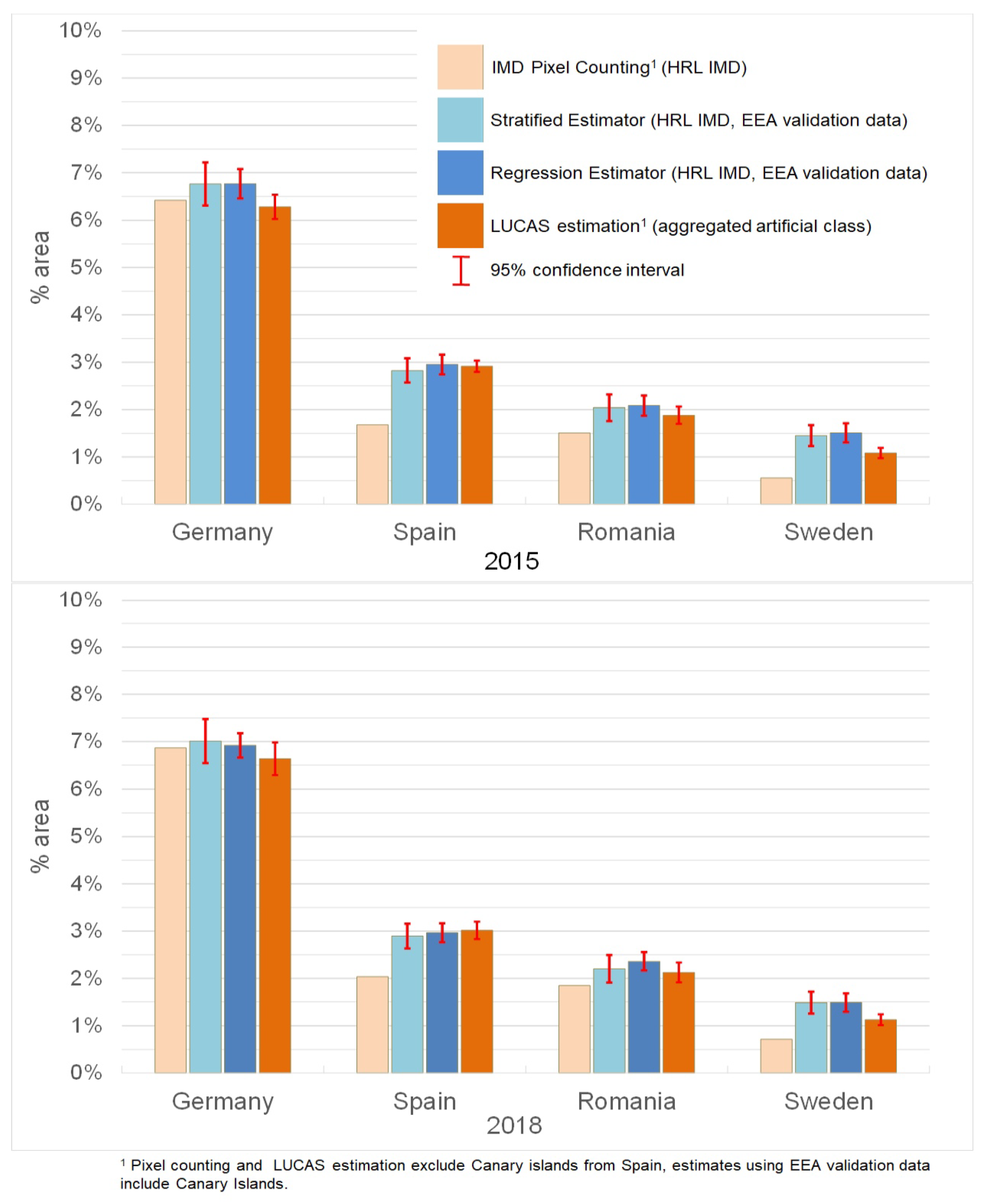
	Pixel Counting (HRL IMD)	Stratified Estimator (EEA Validation Data HRL IMD)	Regression Estimator (EEA Validation Data HRL IMD)	Calibrated Estimator (LUCAS)
	Area %	Area % (CV)	Area % (CV)	Area % (CV)
2015
Germany	6.4	6.8 (3.4)	6.8 (2.3)	6.3 (2.1)
Spain	1.7	2.8 (4.6)	3.0 (3.6)	2.9 (2.1)
Romania	1.5	2.0 (7.0)	2.1 (5.2)	1.9 (4.9)
Sweden	0.6	1.5 (7.8)	1.5 (6.8)	1.1 (5.1)
2018
Germany	6.9	7.0 (3.4)	6.9 (1.9)	6.7 (2.6)
Spain	2.0	2.9 (4.6)	3.0 (3.4)	3.0 (3.1)
Romania	1.8	2.2 (6.6)	2.4 (4.2)	2.1 (5.1)
Sweden	0.7	1.5 (7.8)	1.5 (6.6)	1.1 (5.2)

^a IMD pixel counts and LUCAS estimates exclude Canary islands from Spain; estimates using EEA validation data include Canary Islands.

and Figure 2. The area estimates are compared with an estimation based on the aggregated LUCAS survey data. The uncertainty of the estimates are expressed as coefficient of variation (CV) in Table 5.

In Figure 2, the estimates from 2015 and 2018 are plotted for visual analysis, including the standard error of the estimates at a 95 percent confidence interval expressed as a proportion of the total area. This allows for a better comparison of the estimates and their uncertainty between 2015 and 2018. It shows that the impervious area enumerated by pixel counting of the HRL IMD is generally smaller than the area estimated by the other methods. This applies to both years and all investigated countries, except Germany. Here, the pixel counts are slightly higher than the LUCAS estimates in both years. Only in Germany are the pixel counts within the 95 percent confidence intervals of the other estimates, except for the regression estimator in 2015. The highest differences between area estimates from pixel counting and LUCAS estimation can be seen in both years for Spain and Sweden, where the former provides clearly lower estimates for the impervious area. Estimates using the stratified and regression estimators are similar and close to the LUCAS estimates for Spain and Romania. Sweden and Germany show an overestimation for both years when compared to LUCAS. The CVs of the area estimates are smaller than five percent in Germany and Spain, but higher in Romania and Sweden (except for the Romania 2018 regression estimation). The 2018 estimates for Germany and Romania display an even lower CV for the regression estimator than the aggregated LUCAS class estimate. The differences between the estimates from the stratified estimator and the regression estimator are small and the regression estimator provides slightly higher estimates, with the exception of Germany in 2018.

Country-wide impervious area proportions are higher in 2018 in comparison to 2015, except for Sweden, where the results are almost identical. This increase appears more pronounced in the pixel counting results than in the unbiased estimators and the LUCAS estimate. The proportion of impervious area did not change beyond the 95% confidence interval of the estimates in any of the countries, i.e., the uncertainty of the estimate is higher than the actual change rates themselves. For the simple pixel-counting, no confidence intervals can be provided, which is inherent to the method.

5. Discussion

The stratified and the regression estimators achieved impervious area estimates with CVs of around 5% at a national administrative level. Both approaches were based on the HRL IMD together with (previously unreleased) EEA validation data. Comparable results were achieved by the estimation based on the aggregated LUCAS reference data. Area estimation based on a remote-sensing-derived map via simple pixel counting is problematic, as it can have a very large bias [43], which roughly corresponds to the difference between the commission and the omission errors of the map [44] and does not come with a standard error. The provided EEA validation results showed high differences between user’s and producer’s accuracy for the aggregated IMD product (see Table 2). User’s accuracies were higher in both years and in all selected countries than the producer’s accuracy. This indicates a strong bias and underestimation of impervious area in the IMD products in all countries. The pixel counting results in Germany were similar to the remaining methods, but strongly deviated for the remaining three countries. The Copernicus HRL are standardised products covering all of Europe, and quality and accuracy are likely to vary across the continent. Accuracy information for selected regions or nations are not systematically produced. Recent work indicates that over- and underestimation errors may be more balanced in regions with more built-up land [28], which could explain the closer match of pixel counting results with the other estimation results in Germany. Information on the area of applicability could help to better understand prediction errors [45]. The most recent HRL IMD 2018 was accompanied by a new confidence layer providing information regarding the spatial variability (i.e., at pixel level) of the product quality. The use or applicability of this layer for area estimation could not be assessed due to lacking information on the information content and methodology to create this layer. Future research is needed to include such spatial product quality information in area estimation.

Design-based area estimation approaches require a rigorous probability sampling design to make inferences from a reference sample to the entire population and to allow the calculation of unbiased area estimators with known uncertainty. Such a sample can be costly to produce, and the use of already existing reference data (such as the LUCAS sample) might be seen as a substitute for a dedicated sampling exercise. The LUCAS sampling design is based on NUTS2 level, and allows area estimation down to the NUTS2 level across Europe. Although the LUCAS micro-data are available to the public via the Eurostat website and as further harmonised geodata set [19], estimation of area with the LUCAS data was only possible with the calculated sample weights transferred to areas and provided by Eurostat. Those weights are not yet provided to the public along with the LUCAS micro-data, and not considering these sample weights would introduce a bias in the estimation.

Combining LUCAS data with LCLU maps, such as the HRL IMD for area estimation could be considered to improve area estimation. The redefined LUCAS sampling design, using a ‘dynamic stratification’ process that combines different parameters with the main land cover class from the stratification [31] makes it difficult to apply standard design-based estimators. Conventional stratified estimators as described in [17] cannot be applied because the LUCAS strata are different than the HRL IMD classes. The rows of the population error matrix do not correspond to the strata used to select the sample. Estimators for situations where the stratification of the reference data is different than the map classes are described in [13], but further investigation is required to adequately consider the LUCAS sampling design for unbiased variance estimation.

Another limitation is the spatial comparability of the core LCLU information from LUCAS with EO-based LCLU data. The LUCAS point is defined with a radius of 1.5 m around the point coordinate, and the LCLU observation takes place within this radius. For heterogeneous land cover such as grassland, woodland, wetland, and bare areas, the observation radius is further extended to a 20 m radius around the point (so-called extended window of observation), but only within the same land cover plot where the LUCAS point is located, the so-called “homogeneous plot”. Therefore, the observation unit is not fixed and might not extend to the full 20 m when the point is located close to a land cover border. The spatial resolution of EO-based LCLU maps depends on the resolution of the sensor applied. The HRL IMD is, to a large extent, based on Sentinel-2 with a spatial resolution of 10–20 m (depending on the spectral wavelength used). This limits the spatial comparability of the LUCAS core parameters with the HRL IMD pixels [39] and might lead to a bias when using both data in area estimation. The Copernicus HRL products use the same spatial grid across European as the LUCAS sampling frame, and the LUCAS point is located at the intersection of four HRL product pixels. Therefore, the standard LUCAS observation window (1.5 m radius) relates to four intersecting HRL pixels, not considering any positional inaccuracies of the HRL or the LUCAS observation. Weights (e.g., 0.25, 0.5, 0.75) may be applied when a LUCAS point intersects with different HRL pixel classes.

Other LUCAS survey components have great potential to overcome the current limitations. The Inspire pure land cover components record the proportion of land cover classes in a 20 m radius around the point using a ‘birds eye view’. It was introduced in 2015 and 2018 only for specific land cover classes, and the observation area is limited to the homogeneous plot [34,35]. These limitations are currently addressed in the ongoing 2022 survey. Information on whether the land cover at the point fully covers the 20 m radius or not will be recorded, and the Inspire pure land cover component will be observed at all LUCAS points [18]. The Copernicus Module, first introduced in LUCAS in a pilot stage in 2018, will be extended to 150,000 sample points in the 2022 LUCAS campaign. Provided that the sampling weights of the modules will be available, it could be integrated in future design-based estimation approaches. The imperviousness parameter, also introduced into LUCAS in 2018, applied a different definition than the HRL IMD and recorded information on non-vegetated areas, which may or may not be impervious. It has been renamed in the LUCAS 2022 campaign to “unvegetated area” for better understanding.

The sampling design of the EEA validation data targets thematic map accuracy of the HRL on European level for bio-geographic regions and for large countries or group of countries. Smaller countries, or NUTS2 level, were not considered in the sampling design. The validation data are not publicly available and were provided by the EEA only for this assessment. An direct assessment of the full 20 m or 10 m resolution HRL product was not possible with the existing data. Using a sub-sample of points to estimate the proportion of impervious area in the sample segments is a practical approach, for which implications for comparability are discussed in [46]. Further information on the spatial variation in the product quality, such as the “area of applicability” as proposed by [45], could improve the use of these products for area estimation.

The regression estimator provides precise area estimates and served to further reduce the CV compared to the stratified estimator. This is in particular caused by the high correlation of the IMD values the HRL map and the reference data in the impervious strata.

Estimates based on a reference sample are an extrapolation of accurate observations towards an entire population. The assumption of these approaches is that the reference data provide the “true” and correct information on land cover. Efforts to improve the sampling design and reduce the uncertainty of the estimates are meaningless if errors in the reference data prevail and create non-sampling errors higher than the targeted CV. As shown, there are a number of possible sources of systematic errors related to the reference data or caused by not considering the required comparability between Earth Observation and reference data. These errors are in addition to errors due to wrong classification of the reference data. Errors in the reference data are multiplied towards the entire outcomes, which is why error tracing (sampling/non-sampling errors) and its quantification require crucial attention.

6. Conclusions

Prerequisites for unbiased area estimation are the availability of reference data with adequate probability sampling and sound response design ensuring a match between Earth Observation based maps and reference data. The Copernicus High Resolution Layer products, such as the HRL IMD, could be used for unbiased area estimation, once combined with previously unpublished validation data from the EEA. Compared to a naive estimation approach (pixel counting) using only the Copernicus maps, regression, and stratified estimator methods provided comparable results with specified error rates and in close range to extrapolated LUCAS reference data.

Different sampling designs hinder the direct use of LUCAS data in combination with HRL maps for area estimation using existing standard methods, such as stratified and regression estimators. There is already a strong thematic and temporal match between the Copernicus HRL IMD and the LUCAS program. Adaptations to some LUCAS parameters and modules in the 2022 survey will enable a better uptake of the LUCAS reference data in combination with Copernicus products for area estimation. Using the sample weights provided by Eurostat allowed the calculation of area estimates based on LUCAS alone, important for comparative analysis.

Unbiased area estimation methods combining a map with adequate reference data should be used to generate area statistics. Carefully planned resources for reference data collection and a proper setup of the sampling design will enable good area estimation results within defined uncertainty (range of error) ranges. This study demonstrated that unbiased area estimates are possible using existing pan-European LUCAS and Copernicus HRL maps if:

• Reference data used for the HRL validation are published together with the products;
• The LUCAS sample weights, along with the required information of the sampling design and the stratification applied, are provided for the LUCAS core and Earth-Observation-related modules;
• HRL products are considered for stratification of the LUCAS master frame, and the LUCAS data are used for validation of the HRL products, provided that the methodological continuity of HRL is ensured.

Future applications and research would benefit if:

• Further information on the area of applicability of the underlying classification models is provided to improve the spatial assessment of over- and underestimation,
• HRL products are considered for stratification of the LUCAS master frame and the LUCAS data aew used for validation of the HRL products, provided that the methodological continuity of HRL is ensured;
• The compatibility of the LUCAS survey components with Copernicus HRL products is ensured and improved, which is already the case in the LUCAS 2022 campaign [18].

References

- GFOI. Integration of Remote-Sensing and Ground-Based Observations for Estimation of Emissions and Removals of Greenhouse Gases in Forests: Methods and Guidance from the Global Forest Observations Initiative, 3rd ed.; Global Forest Observations Initiative: Rome, Italy, 2020; Available online: https://www.reddcompass.org/mgd/resources/GFOI-MGD-3.1-en.pdf (accessed on 25 August 2022).
- GSARS. Handbook on Remote Sensing for Agricultural Statistics; Global Strategy to Improve Agricultural and Rural Statistics (GSARS): Rome, Italy, 2017; Available online: https://www.fao.org/3/ca6394en/ca6394en.pdf (accessed on 25 August 2022).
- Stehman, S.V.; Foody, G.M. Key issues in rigorous accuracy assessment of land cover products. Remote Sens. Environ. 2019, 231, 111199. [Google Scholar] [CrossRef]
- EEA. High Resolution Layers, © European Union, Copernicus Land Monitoring Service 2022; European Environment Agency (EEA). 2021. Available online: https://land.copernicus.eu/pan-european/high-resolution-layers/ (accessed on 25 August 2022).
- Gallego, F.J. Copernicus Land Services to Improve EU Statistics; Publications Office of the European Union: Luxembourg, 2017. [CrossRef]
- Gallego, F.J. Remote sensing and land cover area estimation. Int. J. Remote Sens. 2004, 25, 3019–3047. [Google Scholar] [CrossRef]
- Olofsson, P.; Foody, G.M.; Herold, M.; Stehman, S.V.; Woodcock, C.E.; Wulder, M.A. Good practices for estimating area and assessing accuracy of land change. Remote Sens. Environ. 2014, 148, 42–57. [Google Scholar] [CrossRef]
- Foody, G.; Pal, M.; Rocchini, D.; Garzon-Lopez, C.; Bastin, L. The Sensitivity of Mapping Methods to Reference Data Quality: Training Supervised Image Classifications with Imperfect Reference Data. ISPRS Int. J. Geo-Inf. 2016, 5, 199. [Google Scholar] [CrossRef]
- Foody, G. Ground reference data error and the mis-estimation of the Area of land cover change as a function of its abundance. Remote Sens. Lett. 2013, 4, 783–792. [Google Scholar] [CrossRef]
- Benedetti, R.; Bee, M.; Espa, G.; Piersimoni, F. (Eds.) Agricultural Survey Methods; John Wiley & Sons: Chichester, UK, 2010. [Google Scholar] [CrossRef]
- Gallego, J.; Carfagna, E.; Baruth, B. Accuracy, objectivity and efficiency of remote sensing for agricultural statistics. In Agricultural Survey Methods; Benedetti, R., Bee, M., Espa, G., Piersimoni, F., Eds.; John Wiley & Sons: Chichester, UK, 2010; pp. 193–211. [Google Scholar]
- GEOSS. Best Practices for Crop Area Estimation with Remote Sensing; JRC Scientific and Technical Report; Joint Research Centre: Ispra, Italy, 2009; Available online: https://data.europa.eu/doi/10.2788/31835 (accessed on 25 August 2022).
- Stehman, S.V. Estimating area and map accuracy for stratified random sampling when the strata are different from the map classes. Int. J. Remote Sens. 2014, 35, 4923–4939. [Google Scholar] [CrossRef]
- Deville, J.C.; Särndal, C.E. Calibration estimators in survey sampling. J. Am. Stat. Assoc. 1992, 87, 376–382. [Google Scholar] [CrossRef]
- Pengra, B.; Stehman, S.; Horton, J.; Dockter, D.; Schroeder, T.; Yang, Z.; Cohen, W.; Healey, S.; Loveland, T. Quality control and assessment of interpreter consistency of annual land cover reference data in an operational national monitoring program. Remote Sens. Environ. 2019, 238, 111261. [Google Scholar] [CrossRef]
- Stehman, S.V. Basic probability sampling designs for thematic map accuracy assessment. Int. J. Remote Sens. 1999, 20, 2423–2441. [Google Scholar] [CrossRef]
- Cochran, W.G. Sampling Techniques, 3rd ed.; John Wiley & Sons: New York, NY, USA, 1977. [Google Scholar]
- Eurostat. LUCAS–Land Use and Land Cover Survey. 2021. Available online: https://ec.europa.eu/eurostat/statistics-explained/index.php?title=LUCAS_-_Land_use_and_land_cover_survey (accessed on 25 August 2022).
- d’Andrimont, R.; Yordanov, M.; Martinez-Sanchez, L.; Eiselt, B.; Palmieri, A.; Dominici, P.; Gallego, J.; Reuter, H.I.; Joebges, C.; Lemoine, G.; et al. Harmonised LUCAS in-situ land cover and use database for field surveys from 2006 to 2018 in the European Union. Sci. Data 2020, 7, 352. [Google Scholar] [CrossRef]
- Leinenkugel, P.; Deck, R.; Huth, J.; Ottinger, M.; Mack, B. The Potential of Open Geodata for Automated Large-Scale Land Use and Land Cover Classification. Remote Sens. 2019, 11, 2249. [Google Scholar] [CrossRef]
- d’Andrimont, R.; Verhegghen, A.; Lemoine, G.; Kempeneers, P.; Meroni, M.; van der Velde, M. From parcel to continental scale – A first European crop type map based on Sentinel-1 and LUCAS Copernicus in-situ observations. Remote Sens. Environ. 2021, 266, 112708. [Google Scholar] [CrossRef]
- Karydas, C.; Gitas, I.; Kuntz, S.; Minakou, C. Use of LUCAS LC Point Database for Validating Country-Scale Land Cover Maps. Remote Sens. 2015, 7, 5012–5041. [Google Scholar] [CrossRef]
- Gallego, J.; Bamps, C. Using CORINE land cover and the point survey LUCAS for area estimation. Int. J. Appl. Earth Obs. Geoinf. 2008, 10, 467–475. [Google Scholar] [CrossRef]
- Eurostat. NUTS–Nomenclature of Territorial Units for Statistics. 2021. Available online: https://ec.europa.eu/eurostat/web/nuts/background (accessed on 5 September 2022).
- Langanke, T. Copernicus Land Monitoring Service–High Resolution Layer Imperviousness: Product Specifications Document; European Environment Agency: Copenhagen, Denmark, 2016. Available online: https://land.copernicus.eu/user-corner/technical-library/hrl-imperviousness-technical-document-prod-2015 (accessed on 25 August 2022).
- Corbane, C.; Panagiotis, P.; Maffenini, L. MASADA User Guide: Version 2.0; Technical Report; Publications Office of the European Union: Luxembourg, 2019. [Google Scholar]
- EEA. Copernicus Land Monitoring Service. High Resolution Land Cover Characteristics. Lot1: Imperviousness 2018, Imperviousness Change 2015–2018 and Built-Up 2018. User Manual; European Environment Agency: Copenhagen, Denmark, 2018. Available online: https://land.copernicus.eu/user-corner/technical-library//imperviousness-2018-user-manual.pdf (accessed on 25 August 2022).
- Strand, G.H. Accuracy of the Copernicus High-Resolution Layer Imperviousness Density (HRL IMD) Assessed by Point Sampling within Pixels. Remote Sens. 2022, 14, 3589. [Google Scholar] [CrossRef]
- EEA. Copernicus Land Monitoring Service–HRL Imperviousness Degree 2015 Validation Report; GMES Initial Operations/Copernicus Land monitoring services—Validation of Products Third Specific Contract—N°3436/R0- COPERNICUS/EEA.57056; EEA: Copenhagen, Denmark, 2019. Available online: https://land.copernicus.eu/user-corner/technical-library/hrl-imperviousness-2015-validation-report (accessed on 25 August 2022).
- EEA. Copernicus Land monitoring Service–HRL Imperviousness Degree 2018 Validation Report; GMES Initial Operations/Copernicus Land Monitoring Services—Validation of Products Fourth Specific Contract—No 3436/R0- COPERNICUS/EEA.57889; EEA: Copenhagen, Denmark, 2020. Available online: https://land.copernicus.eu/user-corner/technical-library/clms_hrl_imd_validation_report_sc04_1_3.pdf (accessed on 25 August 2022).
- Ballin, M.; Barcaroli, G.; Masselli, M.; Scarnò, M. Redesign Sample for Land Use/Cover Area Frame Survey (LUCAS) 2018; Statistical Working Papers Eurostat; Publications Office of the European Union: Luxembourg, 2018. [CrossRef]
- Gallego, J.; Sannier, C.; Pennec, A. Validation of Copernicus Land Monitoring Services and Area Estimation. In Proceedings of the International Conference of Agricultural Statistics (ICAS), Rome, Italy, 26–28 October 2016; p. 7. Available online: https://land.copernicus.eu/user-corner/technical-library/validation-of-copernicus-land-monitoring-services-and-area-estimation (accessed on 25 August 2022).
- Gallego, J.; Delincé, J. The European land use and cover area-frame statistical survey. In Agricultural Survey Methods; Benedetti, R., Bee, M., Espa, G., Piersimoni, F., Eds.; John Wiley & Sons: Chichester, UK, 2010; pp. 151–168. [Google Scholar]
- Eurostat. LUCAS 2015–Technical Reference Document C1-Instructions for Surveyors; Technical Documents; Eurostat: Luxembourg, 2015.
- Eurostat. LUCAS 2018–Technical reference document C1-Instructions for Surveyors; Eurostat: Luxembourg, 2018.
- d’Andrimont, R.; Verhegghen, A.; Meroni, M.; Lemoine, G.; Strobl, P.; Eiselt, B.; Yordanov, M.; Martinez-Sanchez, L.; van der Velde, M. LUCAS Copernicus 2018: Earth-observation-relevant in situ data on land cover and use throughout the European Union. Earth Syst. Sci. Data 2021, 13, 1119–1133. [Google Scholar] [CrossRef]
- Gallego, F.J. Estimating and correcting the bias of pixel counting. In Handbook on Remote Sensing for Agricultural Statistics; Global Strategy to Improve Agricultural and Rural Statistics (GSARS); GSARS Handbook: Rome, Italy, 2017; pp. 249–257. [Google Scholar]
- Stehman, S. Estimating area from an accuracy assessment error matrix. Remote Sens. Environ. 2013, 132, 202–211. [Google Scholar] [CrossRef]
- Buck, O.; Haub, C.; Woditsch, S.; Lindemann, D.; Kleinewillinghöfer, L.; Hazeu, G.; Kosztra, B.; Kleeschulte, S.; Arnold, S.; Hölzl, M. Task 1.9—Analysis of the LUCAS Nomenclature and Proposal for Adaptation of the Nomenclature in View of Its Use by the Copernicus Land Monitoring Services; Service Contract Report No. 3436/B2015/R0-GIO/EEA.56166; European Environment Agency (EEA): Copenhagen, Denmark, 2015. Available online: https://land.copernicus.eu/user-corner/technical-library/lucas-copernicus-report-2015 (accessed on 25 August 2022).
- Eurostat. LUCAS 2022–Technical Reference Document C2-Field Form (Template); Eurostat: Luxembourg, 2022. Available online: https://ec.europa.eu/eurostat/documents/205002/13686460/C2-LUCAS-2022.pdf (accessed on 25 August 2022).
- Zardetto, D. ReGenesees: An Advanced R System for Calibration, Estimation and Sampling Error Assessment in Complex Sample Surveys. J. Off. Stat. 2015, 31, 177–203. [Google Scholar] [CrossRef]
- Zardetto, D. R Evolved Generalized Software for Sampling Estimates and Errors in Surveys. [Software Code and Documentation]. 2021. Available online: https://www.istat.it/en/methods-and-tools/methods-and-it-tools/process/processing-tools/regenesees (accessed on 25 August 2022).
- Czaplewski, R. Misclassification bias in areal estimates. Photogramm. Eng. Remote Sens. 1992, 58, 189–192. [Google Scholar]
- Carfagna, E.; Gallego, F.J. Using Remote Sensing for Agricultural Statistics. Int. Stat. Rev. 2006, 73, 389–404. [Google Scholar] [CrossRef]
- Meyer, H.; Pebesma, E. Predicting into unknown space? Estimating the area of applicability of spatial prediction models. Methods Ecol. Evol. 2021, 12, 1620–1633. [Google Scholar] [CrossRef]
- Pennec, A.; Sannier, C.; Smith, G. Comparative validation of Artificial Land Products; Technical Report Final Report of the GMES Initial Operations/Copernicus Land Monitoring Services–Validation of Products. Validation Services for the Geospatial Products of the Copernicus Land Continental and Local Components Including In-Situ Data (Lot 1), Third Specific Contract– N°3436/R0-COPERNICUS/EEA.57056; European Environment Agency: Copenhagen, Denmark, 2019. Available online: https://land.copernicus.eu/user-corner/technical-library/comparative-validation-of-artificial-land-products/ (accessed on 25 August 2022).