Article

LS-VCE Applied to Stochastic Modeling of GNSS Observation Noise and Process Noise

1
State Key Laboratory of Geodesy and Earth’s Dynamics, Innovation Academy for Precision Measurement Science and Technology, Chinese Academy of Sciences, Wuhan 430071, China
2
College of Earth and Planetary Sciences, University of Chinese Academy of Sciences, Beijing 100049, China
3
State Key Laboratory of Satellite Navigation System and Equipment Technology, The 54th Research Institute of China Electronics Technology Group Corporation, Shijiazhuang 050081, China
*
Author to whom correspondence should be addressed.
Remote Sens. 2022, 14(2), 258; https://doi.org/10.3390/rs14020258
Submission received: 16 November 2021 / Revised: 1 January 2022 / Accepted: 5 January 2022 / Published: 6 January 2022

Abstract

:
Stochastic models play a crucial role in global navigation satellite systems (GNSS) data processing. Many studies contribute to the stochastic modeling of GNSS observation noise, whereas few studies focus on the stochastic modeling of process noise. This paper proposes a method that is able to jointly estimate the variances of observation noise and process noise. The method is flexible since it is based on the least-squares variance component estimation (LS-VCE), enabling users to estimate the variance components that they are specifically interested in. We apply the proposed method to estimate the variances for the dual-frequency GNSS observation noise and for the process noise of the receiver code bias (RCB). We also investigate the impact of the stochastic model upon parameter estimation, ambiguity resolution, and positioning. The results show that the precision of GNSS observations differs in systems and frequencies. Among the dual-frequency GPS, Galileo, and BDS code observations, the precision of the BDS B3 observations is highest (better than 0.2 m). The precision of the BDS phase observations is better than two millimeters, which is also higher than that of the GPS and Galileo observations. For all three systems, the RCB process noise ranges from 0.5 millimeters to 1 millimeter, with a data sampling rate of 30 s. An improper stochastic model of the observation noise results in an unreliable ambiguity dilution of precision (ADOP) and position dilution of precision (PDOP), thus adversely affecting the assessment of the ambiguity resolution and positioning performance. An inappropriate stochastic model of RCB process noise disturbs the estimation of the receiver clock and the ionosphere delays and is thus harmful for timing and ionosphere retrieval applications.

Graphical Abstract

1. Introduction

Choosing the proper mathematical models, including a functional model, a dynamic model, and a stochastic model, is essential for global navigation satellite systems (GNSS) data processing [1,2]. The functional model describes the relationships between observations and unknown parameters, while the dynamic model specifies the time evolution of unknown parameters [3,4]. A considerable number of studies have established various functional and dynamic models for GNSS positioning, navigation, and timing applications [5,6,7]. However, the stochastic model, which describes the random characteristics of a system, is usually unknown or only partly known. A realistic stochastic model ensures the best linear unbiased estimation, determines an accurate precision description of the unknown parameters, and allows reliable quality control [3,8]. Hence, it is of great importance to establish a realistic stochastic model for GNSS applications.
For stochastic modeling, one must first define the appropriate structure of the covariance matrix. An adequate covariance matrix contains two parts: one for observation noise and another for process noise. Regarding the observation noise, its stochastic properties that reflect the precision of observations, the cross-correlation between different types of observations, and the time correlation of observations can be captured by the covariance matrix [9,10,11]. The stochastic properties of the process noise describe the uncertainty of the dynamic model and should also be properly described by the covariance matrix [8,12]. The correlation between observation noise and process noise is commonly assumed to be zero [8,12].
The covariance matrix is then written as an unknown linear combination of known cofactor matrices [13]. The process of estimating the unknown variance components is referred to as variance component estimation (VCE). Many VCE methods, which tend to differ in estimation principles and distributional assumptions, exist in the literature [14,15,16,17]. This paper focuses on the least-squares variance component estimation (LS-VCE) which is capable of unifying many VCE methods [13,18]. Moreover, it adopts the well-known principle of LS, works with a user-defined weight matrix, and allows one to apply the existing knowledge of LS theories, thus making it simple, flexible, and attractive [13,18].
Many studies have applied the LS-VCE for the stochastic modeling of GNSS observations. Earlier applications of the LS-VCE established a realistic stochastic model for GPS observations [9,19]. Previous studies have also adopted the LS-VCE to analyze the noise characteristics of GPS observations that have been collected by different types of receivers and antennas [10,20,21]. With the emergence of other GNSSs, the LS-VCE contributed to the design of the Chinese BDS a specific stochastic model that considers different variances for geostationary Earth orbit, inclined geosynchronous orbit, and medium Earth orbit satellites [22,23,24]. Galileo multi-frequency observations have also been shown to benefit from a proper stochastic model established by the LS-VCE [25,26,27].
Compared with stochastic modeling of GNSS observation noise, few studies have applied the LS-VCE for the stochastic modeling of process noise. In many applications, knowledge about the process noise for some parameters is still at a rudimentary level. For example, studies in recent years have reported that the receiver code bias (RCB) exhibits short-term variations [28,29,30,31]; however, many studies considered it as a time constant parameter, typically one that is relevant to precise point positioning [32]. RCB is the receiver hardware delay and is composed of contributions from the antenna, cables, amplifiers, and filters. To avoid the adverse effects of RCB variation, one may consider it unlinked in time, with some implementing it in double-differenced real-time kinematic (RTK) positioning, but this results in the model being weaker [33]. The double-differenced RTK positioning eliminates the RCB through differences at each epoch, which is equivalent to modeling the RCB as a time-unlinked parameter. An alternative method is to model the RCB as a random walk process, thus simultaneously ensuring a relatively strong model and capturing RCB variations [34]. However, a realistic stochastic model of the RCB process noise remains to be determined.
Based on the LS-VCE, this paper proposes a method that is able to jointly estimate the variance components for both observation noise and process noise. We first consider the dynamic model as pseudo-observation equations and then integrate them with GNSS observation equations, constructing one covariance matrix that describes both the observation noise and process noise, finally allowing it to be determined through the use of the LS-VCE. To elaborate on the practical aspects of the method, we apply it to jointly estimate the GNSS (GPS+BDS+Galileo) observation noise and the RCB process noise. After the estimates have been validated, we analyze the impact of the stochastic model upon parameter estimation, ambiguity resolution, and positioning.

2. Methods

This section first formulates the general mathematical models that are used for GNSS data processing. The LS-VCE is introduced afterwards. Finally, we present the stochastic modeling method for GNSS observation noise and RCB process noise.

2.1. GNSS Mathematical Models

GNSS mathematical models include a functional model, a dynamic model, and a stochastic model. The functional model describes the relationship between observations and unknown parameters. We write the GNSS functional model as [4]:
y i = A 1 ( i ) x 1 i + A 2 ( i ) x 2 i + ε i
where y i is the observation vector at epoch i ( i = 1 , 2 , . . . , t ), x 1 i is the vector for the unknown parameters that can be further modeled by a dynamic model, while vector x 2 i contains the unknown parameters that are not able to be modeled by a dynamic model. A 1 ( i ) and A 2 ( i ) constitute the full-rank design matrices, and ε i is the vector of random noise. Noting that, we consider a functional model in which not all of the parameters satisfy a dynamic model; this is a common case in GNSS data processing. For example, a dynamic model is usually unavailable for receiver clocks, while carrier-phase ambiguities are considered as time constants in a continuous arc.
The dynamic model describes the time evolution of the state vector x 1 i , and it can be written as [4]:
x 1 i = Φ i , i 1 x 1 i 1 + w i
or
0 = x 1 i + Φ i , i 1 x 1 i 1 + w i
where Φ i , i 1 ( i = 2 , 3 , . . . , t ) is the state transition matrix, and w i is the vector of process noise.
The stochastic model provides the dispersion of random vectors for both the observation noise and process noise, and it can be written as:
D ε i w i = Q ε i 0 0 Q w i
where D . denotes the dispersion operator. We describe the dispersion using a covariance matrix that contains the covariance matrix of observation noise Q ε i and the covariance matrix of process noise Q w i . The covariance between the observation noise and process noise is assumed to be zero.
When multi-epoch data are collected, we consider the state-transition, Equation (3), to be pseudo-observation equations and combine them with the observation, Equation (1), writing the multi-epoch model as:
y = A 1 x 1 + A 2 x 2 + ε 0 = B x 1 + w
where y = y T 1 , y T 2 , . . . , y T t T and A 1 = b l k d i a g A 1 1 , A 1 2 , . . . , A 1 t in which b l k d i a g . denotes the operator of the block diagonal concatenation of the matrices, x 1 = x 1 T 1 , x 1 T 2 , . . . , x 1 T t T , A 2 = b l k d i a g A 2 1 , A 2 2 , . . . , A 2 t , x 2 = x 2 T 1 , x 2 T 2 , . . . , x 2 T t T , ε = ε T 1 , ε T 2 , . . . , ε T t T , w = w T 2 , w T 3 , . . . , w T t T B = b 2 , b 3 , . . . , b t T , in which b i ( i = 2 , 3 , . . . , t ) is a t dimensional column vector whose i t h element is −1 and whose i 1 t h element is Φ i , i 1 , while the other elements are zero.
We formulate the stochastic model for Equation (5) as:
D ε w = Q c o m = b l k d i a g Q ε 1 , Q ε 2 , . . . , Q ε t , Q w 2 , Q w 3 , . . . , Q w t
where Q c o m is the multi-epoch covariance matrix that captures the stochastic properties for both the observation noise and process noise. Assuming that some elements in the covariance matrix Q c o m are unknown, we split the matrix Q c o m into a known part Q 0 and an unknown part:
Q c o m = Q 0 + k = 1 p σ k 2 Q k
where the unknown part contains p variance components σ k 2 with the deterministic cofactor matrix Q k .

2.2. Least-Squares Variance Component Estimation

Equations (5)–(7) establish the general mathematical models for GNSS data processing. However, part of the stochastic model remains to be determined. Many studies have proposed different variance component estimation methods; here, we focus on the LS-VCE method since it is simple, flexible, and attractive [13,18].
LS-VCE is based on the least-squares principle, and its normal equation can be written as [13]:
N σ ^ 2 = L
where σ ^ 2 = σ 1 2 , σ 2 2 , . . . , σ p 2 T is the vector of the unknown variance components. We determine the entries n k l and l k of the p × p matrix N and the p × 1 vector L through:
n k l = 1 2 t r Q k Q c o m 1 P A Q l Q c o m 1 P A l k = 1 2 v T Q c o m 1 Q k Q c o m 1 v 1 2 t r Q k Q c o m 1 P A Q 0 Q c o m 1 P A
where P A = I A A T Q c o m 1 A 1 A T Q c o m 1 is an orthogonal projector and v = P A y c o m is the residual vector. y c o m and A are written as:
y c o m = y 0 , A = A 1 A 2 B 0
which are the observation vector and design matrix in Equation (5), respectively.
Finally, we calculate the unknown variance components through the equation:
σ ^ 2 = N 1 L
In brief summary, Equation (5) combines the functional and dynamic models into a unified framework, making it possible to use one covariance matrix (6) to describe both the observation noise and the process noise. Hence, by means of Equation (7), one can flexibly construct a stochastic model in which the variance components of the observation noise are unknown, those of process noise are unknown, or even both of them are unknown. These unknown variance components can be determined by Equation (11), which is based on the LS-VCE.

2.3. Stochastic Modeling of GNSS Observation Noise and RCB Process Noise

We have already presented the stochastic modeling method of observation noise and process noise. To further elaborate on the method from the practical perspective, we apply the method to estimate the GNSS observation noise and RCB process noise.

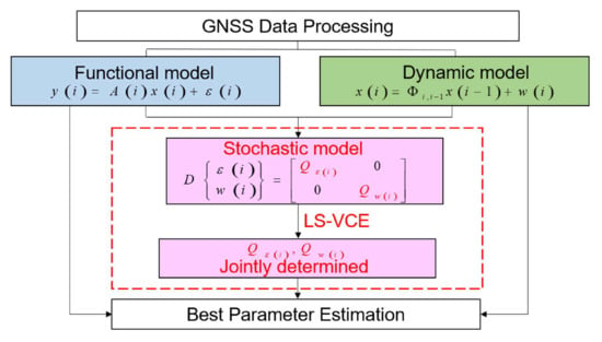
2.3.1. Functional and Dynamic Models

To retrieve the stochastic properties of the pure random noise, one has to eliminate the systematic errors. In an ultra-short or zero baseline, the between-receiver single-differenced (SD) model is almost free of systematic errors and is thus suitable for stochastic modeling [24]. Assuming that the between-receiver SD atmospheric delays are eliminated, we write the full-rank single-epoch SD observation equations at frequency j ( j = 1 , 2 , . . . , f ) for m satellites as [35]:
p j i = ρ i + e m d t ˜ i + e m d ˜ j i + ε p j ( i ) ϕ j i = ρ i + e m d t ˜ i + e m δ ˜ j i + λ j z ˜ j i + ε ϕ j ( i )
where p j i = p j 1 i , p j 2 i , . . . , p j m i T and ϕ j i = ϕ j 1 i , ϕ j 2 i , . . . , ϕ j m i T are the SD code and phase observation vectors, respectively. ρ i = ρ 1 i , ρ 2 i , . . . , ρ m i T is the satellite-to-receiver geometry vector; and z ˜ j i = z ˜ j 2 i , z ˜ j 3 i , . . . , z ˜ j m i T is the integer double-differenced ambiguity vector, in which the coefficient λ j is the wavelength. e m is the m-column vector where all of the elements are ones. ε p j ( i ) = ε p j 1 ( i ) , ε p j 2 ( i ) , . . . , ε p j m ( i ) T is the random noise vector for code observations, while its phase counterpart ε ϕ j ( i ) has the same structure. The parameters denoted by the tildes are not the original parameters but are instead the linear combination of them and are defined in Table 1, where the subscript ‘12’ represents the SD operation between two receivers.
Since the baseline and integer ambiguities can be fixed through the use of long-term observations, we move them to the left side of the equations. Collecting observations of all of the f frequencies yields:
y i   =   e 2 f m I 2 f 1 e m I 2 f e m d t ˜ i γ i ε i
where y i = p T i , ϕ T i T with the observed-minus-calculated code observation vector p i = p 1 T i , p 2 T i , . . . , p f T i T and its phase counterpart ϕ i , I denotes the identity matrix, γ i = d ˜ 2 T i , d ˜ 3 T i , . . . , d ˜ f T i , δ ˜ 1 T i , δ ˜ 2 T i , . . . , δ ˜ f T i T is the vector that contains estimable RCBs and receiver phase bias (RPBs), and ε i = ε p 1 T ( i ) , ε p 2 T ( i ) , . . . , ε p f T ( i ) , ε ϕ 1 T ( i ) , ε ϕ 2 T ( i ) , . . . , ε ϕ f T ( i ) T is the noise vector.
In a multi-epoch case, we integrate the dynamic model with the functional model. We model the estimable receiver clock as white noise and model the receiver code and phase biases as random walk processes, allowing the multi-epoch model to be written as:
y = A 1 γ + A 2 d t ˜ + ε 0 = B γ + w
where we see that Equation (14) has the same structure of Equation (5), but the matrices in Equation (14) are specified for the SD model: A 1 = I t e 2 f m , γ = γ T 1 , γ T 2 , . . . , γ T t T , A 2 = I t I 2 f 1 e m , d t ˜ = d t ˜ T 1 , d t ˜ T 2 , . . . , d t ˜ T t T , and B = b 2 , b 3 , . . . b t T , in which b i ( i = 2 , 3 , . . . , t ) is a t dimensional column vector whose i t h element is −1 and whose i 1 t h element is 1, while the other elements are zero.

2.3.2. Formulation of the Stochastic Model

Following the structure in Equation (6), we are able to formulate the covariance matrix for the SD model as:
Q S D = b l k d i a g Q ε , Q w Q ε = I t b l k d i a g C p , C ϕ H m Q w = I t 1 C w
where C p = d i a g σ p 1 2 , . . . , σ p f 2 and C ϕ = d i a g σ ϕ 1 2 , . . . , σ ϕ f 2 with σ p j 2 and σ ϕ j 2 are the variances for code and phase observation noise. C w = d i a g σ d 2 2 , . . . , σ d f 2 , σ δ 1 2 , . . . , σ δ f 2 with σ d j 2 and σ δ j 2 are the variances of the random walk noise for the receiver code and phase biases. H m = d i a g h 1 , . . . , h m captures the elevation-dependent precision of the observations, which can be given as [36]:
h m = 1 + 10 exp θ m 10 2
where θ m is the satellite elevation in degrees.

2.3.3. Estimation of Variances for Observation Noise and Process Noise

To jointly estimate the variances for the observation noise and process noise, we split, following Equation (7), the covariance matrix in Equation (15) into several variance components:
Q S D = k = 1 p = 4 f 1 σ k 2 Q k
where σ k 2 contains 2 f variance components for the observation noise and 2 f 1 variance components for the process noise of receiver biases. Their cofactor matrices are:
Q k = b l k d i a g I t b l k d i a g 0 m * ( k 1 ) , H m , 0 m * ( 2 f k ) , Q w f o r   k = 1 , . . . , 2 f Q k = b l k d i a g Q ε , I t b l k d i a g I k 2 f 1 , 1 , I 4 f k 1   f o r k = 2 f + 1 , . . . , 4 f 1
where 0 m * ( k 1 ) is a zero matrix of m rows and k 1 columns.
After the construction of the normal equations of the LS-VCE by using Equation (9), one can jointly estimate the variances for both the GNSS observation noise and process noise. Experiments will be conducted in the next section, and certain computational problems that may arise will be discussed.

3. Experiments and Results

This section first introduces the experimental setup. We will then analyze the characteristics of the RCBs and RPBs. After showing the estimated variances of the GNSS observation noise and RCB process noise, we validate the estimates and investigate the impact of the stochastic model on parameter estimation in RTK positioning.

3.1. Experiment Setup

Figure 1 shows the experimental setup. The measurement campaign consists of one zero baseline and two ultra-short baselines. Zero (or ultra-short) baselines are commonly used configurations for stochastic modeling since most of the systematic errors (e.g., the multipath) can be eliminated [9,24,37]. In the zero baseline IGG2–IGG3, a Septentrio PolarX5S receiver and a Trimble Alloy receiver were connected to a common antenna. Another antenna was connected to a Septentrio PolarX5S receiver that was 3.2 m away, resulting in the construction of two short baselines: IGG1-IGG2 and IGG1-IGG3. All three receivers collected dual-frequency GPS (L1/L2) [38], Galileo (E1/E5a) [39], and BDS (B1/B3) observations from DOY (day of year) 268 to 270, 2019. The data sampling rate was 30 s. In this experiment, the BDS refers to the third-generation global BeiDou navigation satellite system [40]. We excluded the GLONASS system since its observations are affected by the inter-frequency biases, which should to be calibrated before stochastic modeling [41]. We will use the data on DOY 268 to conduct stochastic modeling and use the data on DOY 269 and DOY 270 to validate the established stochastic models. Studies have demonstrated that one-day data are enough for stochastic modeling [9,24].

3.2. Characteristics of Receiver Biases

Several studies have reported that receiver biases exhibit short-term variations, which are receiver and antenna specific [28,29,30,31]. This section will show the characteristics of the receiver biases that are involved in the data that we collected.
Figure 2 shows the time series of the Galileo RCB. We estimated the RCB in a filtering process and considered the RCB as white noise. The Galileo RCB exhibits variations between –3.6 m to –2.6 m. This confirms the findings that were reported in other studies, which indicated that the RCB varies over the course of a day [28,29,30,31]. Hence, it is unsuitable to model the RCBs as time constants. One may opt to model the RCB as white noise, but this results in the model becoming weaker. One of the methods that is preferable is to model the RCB as a random walk process, provided that the realistic stochastic model of the random-walk noise can be determined.
Figure 3 shows the time series of the GPS L1 RPB. The RPB also shows intra-day variations. Reviewing the definition of RPB that is given in Table 1, the estimable RPB absorbs the RCB at the first frequency. Hence, the RPB time series contains RCB variations and the RCB variations may even dominate the time series. To further investigate this, we turn to Figure 4.
Figure 4 shows the time series of the BDS RCB and the RPB at two different frequencies. The characteristics of the RPB at the two different frequencies are virtually the same. Moreover, the RPB and RCB exhibit similar properties. This further demonstrates that the RCB that is absorbed in the estimable RPB dominates the RPB time series. In other words, all three time series in Figure 4 actually reflect the characteristics of the RCB.

3.3. Variances of GNSS Observation Noise and RCB Process Noise

This section shows the estimated variances of observation noise and RCB process noise. Since the characteristics of the RCB and the RPB at two frequencies were demonstrated to be almost the same, we estimated the same variance for all of them. Since the phase observation precision is much higher than that of the code one, the LS-VCE model may encounter an ill-posed problem. To handle this problem, we followed the strategy in [18] and estimated one same variance for the dual-frequency phase observations. To improve the computational efficiency, we divided the observations into 10-epoch groups, with the final estimates being the means of the 10-epoch estimates [18]. For each group, we estimated the variance component iteratively. The a priori values for code observation noise, phase observation noise, and RCB process noise were set to 0.3 m, 0.003 m, and 0.03 m, respectively. The estimation procedure could be convergent after several (about three to five) iterations.
Figure 5 shows the standard deviations (STDs) of the GPS, Galileo, and BDS SD code observation noise at the first frequency. The STDs of the GPS and Galileo SD code observations are approximately 0.2 m, while the BDS observations are noisier, with STDs of approximately 0.3 m. This indicates that the observation precision differs between systems, which confirms the findings of other studies [10]. The BDS results are absent for a while (UTC hour 12 to 14) since less than four satellites are tracked at that time, making reliable estimates unavailable.
Figure 6 shows the STD of the GPS, Galileo, and BDS SD phase observation noise. The precision of the GPS SD phase observation is approximately 2 millimeters, while the precision of the Galileo SD phase observation can reach 3 millimeters. As for BDS, most of the estimates are under 2 millimeters, indicating that the precision of the BDS phase observations is the highest. The precision of the phase observations is also system specific. Hence, it is critical to establish a realistic stochastic model for each system rather than use one empirical stochastic model for all systems.
Figure 7 shows the estimates of variance components for the RCB process noise. The results indicate that the STD of the RCB process noise is at the sub-millimeter level for all three systems. Such small process noise results in a stronger model compared with a model that considers the RCB as white noise. On the other hand, this random walk noise can capture RCB variations, instead of incorrectly constraining the RCB as a time constant. One may question why the process noise shown in Figure 7 is so small, whereas the RCB time series shown in Figure 2 seems to be much noisier. This is because Figure 7 shows the final estimates with several iterations, while Figure 2 shows the RCB time series calculated by considering the RCB unlinked in time, which are equivalent to the one-iteration results that are not convergent and need further calculations.
Table 2 provides all of the estimated STDs of the GPS, Galileo, and BDS observation noise and of the RCB process noise for all three baselines. The results indicate that the precision of observations differs in systems and frequencies. For example, the precision of the Galileo code observations is higher than that of the GPS observations. The BDS B1 code observation is noisier than the BDS B3 code observation. We also see that observations that are collected by different baselines exhibit inhomogeneous precision; this is because the observation quality is related to receivers [20]. The STDs of triple-system RCB process noises are all at the sub-millimeter level at three baselines.

3.4. Validation and Impact of the Stochastic Model

This section aims to validate the stochastic model that was estimated in the last section and to investigate the impact of the stochastic model. We will first focus on the stochastic model of the observation noise and then turn to that of RCB process noise.
To validate the stochastic model of the observation noise, we verify whether the actual precision of RTK positioning matches its formal precision. Here, we refer to the positioning as the ionosphere-fixed RTK in which the between-receiver single-differenced ionosphere delays are assumed to be absent [35]. The actual precision refers to the one calculated by the positioning errors, while the formal precision comes from the covariance matrix that was generated by the least-squares estimator.
Figure 8 shows the RTK positioning using a realistic and an empirical stochastic model. Here, we conducted the RTK positioning in an epoch-by-epoch manner. The empirical stochastic model sets the STDs of code and phase observations as 0.3 m and 3 mm, respectively, and ignores the system-specific and frequency-specific precision. We see that the actual and formal confidence intervals match well when the previously estimated stochastic model is used, indicating that the stochastic model we estimated reflects the realistic precision of observations. However, in the case of an empirical stochastic model, the formal intervals are far away from the actual intervals, indicating that the realistic precision of the observations is higher than the empirical value.
To further investigate the impact of the stochastic model upon ambiguity resolution, Figure 9 shows the ambiguity dilution of precision (ADOP) of the positioning using a realistic and an empirical stochastic model. We see that the ADOP with a realistic stochastic model is much smaller than the ADOP with an empirical one. As the ADOP reveals the formal precision of ambiguities, one can use it as an indicator to decide whether or not to fix the ambiguities or which ambiguities should be fixed. Hence, the unreliable ADOP that is calculated by the unrealistic stochastic model will adversely affect the ambiguity resolution process. We note that, if the empirical values are chosen to be smaller than the realistic values, the ADOP based on the empirical value will be smaller. However, this does not mean that the ambiguity resolution based on the empirical stochastic model will perform better. On the contrary, the smaller ADOP based on the empirical stochastic model indicates that the precision of the ambiguities is overestimated, which would result in incorrect ambiguity resolution [24].
We then validate the STD of RCB process noise that we estimated before. For this purpose, we processed the data in a filtering way and verified whether the residuals of the RCB dynamic model satisfied a zero-mean normal distribution. These RCB residuals were calculated by differencing the RCB estimates in two consecutive epochs. We also verified the consistency between the formal RCB process noise and the actual RCB process noise. The formal RCB process noise refers to the one configured in the filtering process. Here, we set it to 10 m, 0.74 millimeters (estimated before), and 0.001 millimeters, respectively. The actual RCB process noise refers to the STD of the RCB residuals. Figure 10 shows that although the RCB residuals based on three different stochastic models all obey normal distribution, only the results based on our estimated stochastic model exhibit the consistency between formal RCB process noise and actual RCB process noise, which validates the correctness of the stochastic model of the RCB process noise we established.
We then investigate how the stochastic model of the RCB process noise affected the parameter estimation. Figure 11 shows the ADOP, PDOP, and receiver clock precision of the ionosphere-fixed RTK positioning with a realistic and an empirical stochastic model of the RCB process noise. The results indicate that the baseline and ambiguity estimation are insensitive to the RCB stochastic model. However, the RCB stochastic model affects the estimation of the receiver clock, as the formal precision is larger when it is paired with an empirical stochastic model than it is when it is paired with a realistic one. This is because the estimable receiver clock absorbs the RCB, while the baseline and ambiguities are independent of the RCB.
To investigate the impact of the RCB stochastic model upon the ionosphere estimation, we switched the ionosphere-fixed RTK model to the ionosphere-weighted one in which the ionosphere delays are estimated [35]. Figure 12 shows the receiver clock and ionosphere precision in GPS+BDS+Galileo dual-frequency ionosphere-weighted RTK positioning. Except for the receiver clock, the stochastic model of the RCB process noise also affects the ionosphere estimation. Hence, an unrealistic stochastic model of RCB process noise will affect the applications such as timing and ionosphere retrieval.

4. Discussion

In the literature, many studies analyzed the stochastic properties of GNSS observation noise [9,10,20], whereas investigations on the process noise are relatively limited. In this contribution, we proposed a method that is able to jointly estimate the variances of GNSS observation noise and RCB process noise, thereby establishing a realistic stochastic model. By comparing our realistic stochastic model with the empirical stochastic model that is commonly adopted in RTK positioning, we analyzed the impact of the stochastic model on parameter estimation, ambiguity resolution, and positioning.
We focused on the RCB process noise since its stochastic model adopted in many applications is needed to be refined. RCB has long been identified as a time constant parameter in precise point positioning [7,32]. However, many studies that have been published in recent years reported that the RCB exhibits short-term variations [28,29,30]. Our results (in Figure 2, Figure 3 and Figure 4) also confirmed this finding. To avoid the adverse impact of RCB variations, double-differenced RTK positioning considers the RCB as a time-unlinked parameter, but this results in the model becoming weaker [26]. We suggest modeling the RCB as a random walk process that is accompanied by a proper stochastic model. The results (in Figure 7 and Table 2) indicated that the estimated RCB process noise is at the submillimeter level. Applying this realistic process noise into the positioning could create optimal parameter estimation, provided that the stochastic model of GNSS observations is also proper.
Figure 8 and Figure 9 illustrated that the stochastic model of the GNSS observations affects the performance assessment of the positioning and ambiguity resolution. Other studies have demonstrated that an improper stochastic model of observation noise could adversely affect the quality control and deteriorate the positioning performance [24]. As far as the RCB process noise is concerned, previous studies have stated that an improper stochastic model of the RCB process noise could affect parameter estimation [34], while this contribution further clarified which parameters would be affected. As shown in Figure 11 and Figure 12, the stochastic model of the RCB process noise affects the estimation of the ionospheric delay and receiver clock, while the receiver coordinates and ambiguities are insensitive to the stochastic model of RCB process noise.

5. Conclusions

A proper stochastic model is the prerequisite to obtain the best linear unbiased estimation in global navigation satellite systems (GNSS) data processing. This paper proposed a method that is able to jointly estimate the variances for both the observation noise and process noise by using the least-squares variance component estimation (LS-VCE). We applied the proposed method to estimate the observation noise of GPS, BDS, and Galileo, as well as the process noise of the receiver code bias (RCB). We also investigated the impact of the stochastic model upon parameter estimation, ambiguity resolution, and positioning. The main findings and conclusions are discussed below.
The precision of GNSS observations differs in terms of both systems and frequencies. For example, the precision of the Galileo E1 code observation is 0.14 m to 0.21 m, which is higher than that of the GPS and BDS observations at the first frequency. The precision of the BDS B3 code observations is better than 0.2 m, which is higher than its B1 counterpart. The precision of the phase observations also differs, and the BDS phase observations enjoy the highest precision (better than two millimeters) among the three systems. The RCB process noise ranges from 0.5 millimeters to 1 millimeter for all three systems, with a data sampling rate of 30 s.
The stochastic model of observation noise affects the ambiguity resolution and the performance assessment of the positioning. The ambiguity dilution of precision (ADOP) based on the realistic stochastic model is much smaller than that calculated through the use of an empirical stochastic model, indicating that an improper stochastic model affects the predictor for ambiguity resolution performance, which may lead to wrong decisions being made to fix the ambiguities. The formal precision of the positioning matches well with the actual precision when using a realistic stochastic model, while the formal precision is far from the actual precision that is achieved when using an empirical stochastic model. This illustrates that an inappropriate stochastic model affects the assessment of the positioning performance.
The stochastic model of the RCB process noise affects the estimation of the receiver clock and ionosphere delays. The residuals of the RCB dynamic model satisfy a zero-mean normal distribution and the standard deviation (STD) of the residuals is consistent with the process noise that we estimated, thus demonstrating the reliability of the stochastic model. Although the position dilution of precision (PDOP) and ADOP are insensitive to the stochastic model of the process noise, the formal precision of the receiver clock and ionosphere delays are affected. This is because the estimable receiver clock and ionosphere delay absorbs RCB, while the baseline and ambiguities are independent of RCB. Hence, an improper stochastic model of the RCB process noise will adversely affect the timing and ionosphere retrieval applications.
In this paper, we applied the proposed method to jointly estimate the variances of GNSS observation noise and RCB process noise. The method is generally applicable and allows the variances of observation noise and process noise to be estimated according to one’s specific needs and interests. The analysis of this paper is limited to 30 s GNSS observations, one can also use the proposed method to analyze high-rate (e.g., 10 s, 5 s, or 1 s) data.

Author Contributions

Conceptualization, J.Z. and B.Z; methodology, J.Z. and P.H.; software, P.H.; validation, P.H., J.Z., T.L., and B.Z.; formal analysis, J.Z.; investigation, P.H.; resources, B.Z.; data curation, P.H.; writing—original draft preparation, P.H.; writing—review and editing, J.Z. and B.Z.; visualization, T.L.; supervision, B.Z.; project administration, B.Z. and T.L.; funding acquisition, B.Z. and T.L. All authors have read and agreed to the published version of the manuscript.

Funding

This research was funded by the Key Research and Development Plan of Hubei Province (Grant Number: 2020BHB014), the National Natural Science Foundation of China (Grant Number: 42174034), and the Scientific Instrument Developing Project of the Chinese Academy of Sciences (Grant Number: YJKYYQ20190063). The fourth author is supported by the CAS Pioneer Hundred Talents Program.

Data Availability Statement

The datasets that support the findings of this research are available from the corresponding author on reasonable request.

Conflicts of Interest

The authors declare no conflict of interest.

References

  1. Leick, A.; Rapoport, L.; Tatarnikov, D. GPS Satellite Surveying, 4th ed.; Wiley: Hoboken, NJ, USA, 2015; ISBN 978-1-118-67557-1. [Google Scholar]
  2. Teunissen, P.J.G.; Kleusberg, A. GPS for Geodesy, 2nd ed.; Springer: Berlin/Heidelberg, Germany, 1998. [Google Scholar]
  3. Koch, K.-R. Parameter Estimation and Hypothesis Testing in Linear Models; Springer: Berlin/Heidelberg, Germany, 1999. [Google Scholar]
  4. Teunissen, P.J.G.; Montenbruck, O. Springer Handbook of Global Navigation Satellite Systems; Springer International Publishing: Cham, Switzerland, 2017. [Google Scholar]
  5. Morton, Y.J.; van Diggelen, F.; Spilker, J.J., Jr.; Parkinson, B.W.; Lo, S.; Gao, G. Position, Navigation, and Timing Technologies in the 21st Century: Integrated Satellite Navigation, Sensor Systems, and Civil Applications; John Wiley & Sons: Hoboken, NJ, USA, 2021. [Google Scholar]
  6. Wübbena, G.; Schmitz, M.; Bagge, A. PPP-RTK: Precise point positioning using state-space representation in RTK networks. In Proceedings of the ION GNSS 2005, The Institute of Navigation, Long Beach, CA, USA, 13–16 September 2005; pp. 2584–2594. [Google Scholar]
  7. Zumberge, J.F.; Heflin, M.B.; Jefferson, D.C.; Watkins, M.M.; Webb, F.H. Precise point positioning for the efficient and robust analysis of GPS data from large networks. J. Geophys. Res. Earth Surf. 1997, 102, 5005–5017. [Google Scholar] [CrossRef] [Green Version]
  8. Teunissen, P.J.G. Adjustment theory: An introduction; VSSD, Delft University Press: Delft, The Netherlands, 2000. [Google Scholar]
  9. Amiri-Simkooei, A.R.; Teunissen, P.J.G.; Tiberius, C. Application of Least-Squares Variance Component Estimation to GPS Observables. J. Surv. Eng. 2009, 135, 149–160. [Google Scholar] [CrossRef] [Green Version]
  10. Bona, P. Precision, Cross Correlation, and Time Correlation of GPS Phase and Code Observations. GPS Solut. 2000, 4, 3–13. [Google Scholar] [CrossRef]
  11. de Bakker, P.F.; Tiberius, C.C.; van der Marel, H.; van Bree, R.J. Short and zero baseline analysis of GPS L1 C/A, L5Q, GIOVE E1B, and E5aQ signals. GPS Solut. 2012, 16, 53–64. [Google Scholar] [CrossRef] [Green Version]
  12. Teunissen, P. Testing Theory; VSSD, Delft University Press: Delft, The Netherlands, 2006. [Google Scholar]
  13. Teunissen, P.J.G.; Amiri-Simkooei, A.R. Least-squares variance component estimation. J. Geod. 2007, 82, 65–82. [Google Scholar] [CrossRef] [Green Version]
  14. Koch, K.R. Maximum likelihood estimate of variance components. J. Geod. 1986, 60, 329–338. [Google Scholar] [CrossRef]
  15. Kubik, K. The estimation of the weights of measured quantities within the method of least squares. Bull. Géodésique 1970, 95, 21–40. [Google Scholar] [CrossRef]
  16. Kusche, J. A Monte-Carlo technique for weight estimation in satellite geodesy. J. Geod. 2003, 76, 641–652. [Google Scholar] [CrossRef] [Green Version]
  17. Rao, C. Estimation of variance and covariance components—MINQUE theory. J. Multivar. Anal. 1971, 1, 257–275. [Google Scholar] [CrossRef] [Green Version]
  18. Amiri-Simkooei, A. Least-Squares VarianceComponent Estimation: Theory and GPS Applications. Ph.D. Thesis, Delft University of Technology, Delft, The Netherlands, 2007. [Google Scholar]
  19. Amiri-Simkooei, A.; Zangeneh-Nejad, F.; Asgari, J. Least-squares variance component estimation applied to GPS geome-try-based observation model. J. Surv. Eng. 2013, 139, 176–187. [Google Scholar] [CrossRef]
  20. Li, B.; Shen, Y.; Xu, P. Assessment of stochastic models for GPS measurements with different types of receivers. Sci. Bull. 2008, 53, 3219–3225. [Google Scholar] [CrossRef] [Green Version]
  21. Zhang, B.; Hou, P.; Liu, T.; Yuan, Y. A single-receiver geometry-free approach to stochastic modeling of multi-frequency GNSS observables. J. Geod. 2020, 94, 1–21. [Google Scholar] [CrossRef]
  22. Hou, P.; Zhang, B.; Yuan, Y. Combined GPS+BDS instantaneous single- and dual-frequency RTK positioning: Stochastic modelling and performance assessment. J. Spat. Sci. 2019, 66, 3–26. [Google Scholar] [CrossRef]
  23. Hou, P.; Zhang, B.; Yuan, Y.; Zhang, X.; Zha, J. Stochastic modeling of BDS2/3 observations with application to RTD/RTK positioning. Meas. Sci. Technol. 2019, 30, 095002. [Google Scholar] [CrossRef]
  24. Li, B. Stochastic modeling of triple-frequency BeiDou signals: Estimation, assessment and impact analysis. J. Geod. 2016, 90, 593–610. [Google Scholar] [CrossRef]
  25. Hu, H.; Xie, X.; Gao, J.; Jin, S.; Jiang, P. GPS-BDS-Galileo double-differenced stochastic model refinement based on least-squares variance component estimation. J. Navig. 2021, 74, 1381–1396. [Google Scholar] [CrossRef]
  26. Odolinski, R.; Teunissen, P.J. Low-cost, 4-system, precise GNSS positioning: A GPS, Galileo, BDS and QZSS iono-sphere-weighted RTK analysis. Meas. Sci. Technol. 2017, 28, 125801. [Google Scholar] [CrossRef] [Green Version]
  27. Zaminpardaz, S.; Teunissen, P.J.G. Analysis of Galileo IOV + FOC signals and E5 RTK performance. GPS Solut. 2017, 21, 1855–1870. [Google Scholar] [CrossRef]
  28. Mi, X.; Sheng, C.; El-Mowafy, A.; Zhang, B. Characteristics of receiver-related biases between BDS-3 and BDS-2 for five fre-quencies including inter-system biases, differential code biases, and differential phase biases. GPS Solut. 2021, 25, 1–11. [Google Scholar] [CrossRef]
  29. Zha, J.; Zhang, B.; Yuan, Y.; Zhang, X.; Li, M. Use of modified carrier-to-code leveling to analyze temperature dependence of multi-GNSS receiver DCB and to retrieve ionospheric TEC. GPS Solut. 2019, 23, 1–12. [Google Scholar] [CrossRef]
  30. Zhang, B.; Teunissen, P.J.G. Characterization of multi-GNSS between-receiver differential code biases using zero and short baselines. Sci. Bull. 2015, 60, 1840–1849. [Google Scholar] [CrossRef] [Green Version]
  31. Zhang, Z.; Yuan, H.; Li, B.; He, X.; Gao, S. Feasibility of easy-to-implement methods to analyze systematic errors of multipath, differential code bias, and inter-system bias for low-cost receivers. GPS Solut. 2021, 25, 1–14. [Google Scholar] [CrossRef]
  32. Zhang, B.; Zhao, C.; Odolinski, R.; Liu, T. Functional model modification of precise point positioning considering the time-varying code biases of a receiver. Satell. Navig. 2021, 2, 1–10. [Google Scholar] [CrossRef]
  33. Teunissen, P.J.G. A canonical theory for short GPS baselines. J. Geod. 1997, 71, 320–336. [Google Scholar] [CrossRef]
  34. Teunissen, P.; Khodabandeh, A.; Psychas, D. A generalized Kalman filter with its precision in recursive form when the sto-chastic model is misspecified. J. Geod. 2021, 95, 1–12. [Google Scholar] [CrossRef]
  35. Odolinski, R.; Teunissen, P.J.G.; Odijk, D. Combined GPS + BDS for short to long baseline RTK positioning. Meas. Sci. Technol. 2015, 26. [Google Scholar] [CrossRef]
  36. Eueler, H.-J.; Goad, C.C. On optimal filtering of GPS dual frequency observations without using orbit information. J. Geod. 1991, 65, 130–143. [Google Scholar] [CrossRef]
  37. Zhang, Z. Code and phase multipath mitigation by using the observation-domain parameterization and its application in five-frequency GNSS ambiguity resolution. GPS Solut. 2021, 25, 1–14. [Google Scholar] [CrossRef]
  38. Barnes, D. GPS Status and Modernization. Presentation at Munich Satellite Navigation Summit. 2019. Available online: https://apps.dtic.mil/dtic/tr/fulltext/u2/a550403.pdf (accessed on 22 December 2021).
  39. Benedicto, J. Directions 2020: Galileo moves ahead. GPS World 2019, 30, 38–47. [Google Scholar]
  40. CSNO. Development of the BeiDou Navigation Satellite System (Version 4.0). 2019. Available online: http://www.beidou.gov.cn/xt/gfxz/201912/P020191227430565455478.pdf (accessed on 22 December 2021).
  41. Zrinjski, M.; Barković, Đ.; Matika, K. Development and Modernization of GNSS. Geod. List 2019, 73, 45–65. [Google Scholar]
Figure 1. One zero baseline (IGG2–IGG3) and two short baselines (IGG1–IGG2, IGG1–IGG3) using three receivers.
Remotesensing 14 00258 g001
Figure 2. Time series of the Galileo RCB calculated using the IGG1–IGG2 baseline data collected on DOY 268, 2019.
Remotesensing 14 00258 g002
Figure 3. Time series of the GPS L1 RPB calculated using the IGG1–IGG2 baseline data collected on DOY 268, 2019.
Remotesensing 14 00258 g003
Figure 4. Time series of the BDS RCB and RPB at two frequencies calculated using the IGG1–IGG2 baseline data collected on DOY 268, 2019.
Remotesensing 14 00258 g004
Figure 5. Estimated STD of the GPS, Galileo, and BDS SD code observation noise at the first frequency calculated using the IGG1–IGG2 baseline data collected on DOY 268, 2019.
Remotesensing 14 00258 g005
Figure 6. Estimated STD of the GPS, Galileo, and BDS SD phase observation noise calculated using the IGG1–IGG2 baseline data collected on DOY 268, 2019.
Remotesensing 14 00258 g006
Figure 7. Estimated STD of the GPS, Galileo, and BDS RCB process noise calculated using the IGG1–IGG2 baseline data collected on DOY 268, 2019.
Remotesensing 14 00258 g007
Figure 8. GPS+BDS+Galileo dual-frequency ionosphere-fixed RTK positioning errors with a realistic (left) and an empirical (right) stochastic model. The green and red lines represent the actual and formal 95% confidence intervals, respectively. The data were collected from baseline IGG1–IGG2 on DOY 269, 2019.
Remotesensing 14 00258 g008
Figure 9. ADOP of GPS+BDS+Galileo dual-frequency ionosphere-fixed RTK positioning with a realistic and an empirical stochastic model. The data were collected from baseline IGG1–IGG2 on DOY 269, 2019.
Remotesensing 14 00258 g009
Figure 10. BDS RCB residuals with the STDs of the process noise set to 10 m (top), 0.74 mm (middle), and 0.001 mm (bottom). The data were collected from baseline IGG1–IGG2 on DOY 270, 2019.
Remotesensing 14 00258 g010
Figure 11. ADOP, PDOP, and clock precision in GPS+BDS+Galileo dual-frequency ionosphere-fixed RTK positioning with a realistic and an empirical stochastic model of RCB process noise. The empirical stochastic model refers to the one that sets the STD of RCB process noise as 10 m. The data were collected from baseline IGG1–IGG2 on DOY 270, 2019.
Remotesensing 14 00258 g011
Figure 12. Clock and ionosphere precision in GPS+BDS+Galileo dual-frequency ionosphere-weighted RTK positioning with a realistic and an empirical stochastic model of RCB process noise. The empirical stochastic model refers to the one that sets the STD of RCB process noise as 10 m. The data were collected from the baseline IGG1–IGG2 on DOY 270, 2019.
Remotesensing 14 00258 g012
Table 1. Estimable parameters of between-receiver single-differenced model.
Estimable ParameterNotation and Interpretation
Receiver clock d t ˜ i = d t 12 i d 12 , 1 i
Receiver code bias d ˜ j i = d 12 , j i d 12 , 1 i j > 1
Receiver phase bias δ ˜ j i = δ 12 , j i d 12 , 1 i + λ j z 12 , j 1 i
Integer ambiguity z ˜ j m i = z 12 , j m i z 12 , j 1 i
Table 2. Estimated STDs of the GPS, Galileo, and BDS observation noise and of the RCB process noise for three baselines.
BaselineSystemRCB (mm)Code 1 (m) Code 2 (m) Phase (mm)
IGG1–IGG2GPS0.610.210.262.01
Galileo0.690.170.232.57
BDS0.740.310.131.73
IGG1–IGG3GPS0.620.380.352.35
Galileo0.700.210.262.89
BDS0.610.360.171.93
IGG2–IGG3GPS0.750.340.271.52
Galileo0.830.140.242.39
BDS0.810.310.121.27
Publisher’s Note: MDPI stays neutral with regard to jurisdictional claims in published maps and institutional affiliations.

